A High Spatiotemporal Resolution Global Gridded Dataset of Historical Human Discomfort Indices

Abstract

Meteorological human discomfort indices or bioclimatic indices are important metrics to gauge potential risks to human health under varying environmental thermal exposures. Derived using sub-daily meteorological variables from a quality-controlled reanalysis data product (Global Land Data Assimilation System—GLDAS), a new high-resolution global dataset referred to as “HDI_0p25_1970_2018” is presented in this study. The dataset includes the following daily indices at 0.25° × 0.25° gridded resolution: (i) Apparent Temperature indoors (AT_ind); (ii) two variants of Apparent Temperature outdoors in shade (AT_ot); (iii) Heat Index (HI); (iv) Humidex (HDEX); (v) Wet Bulb Temperature (WBT); (vi) two variants of Wet Bulb Globe Temperature (WBGT); (vii) Thom Discomfort Index (DI); and (viii) Windchill Temperature (WCT). Spanning 49 years over the period 1970–2018, HDI_0p25_1970_2018 fills gaps in existing climate indices datasets by being the only high-resolution historical global-gridded daily time-series of multiple human discomfort indices based on different meteorological parameters, thus offering applications in wide-ranging climate zones and thermal-comfort environments.

1. Introduction

Recent global temperature extremes, such as the summer heatwaves in Europe (2003, 2006, 2018, and 2019), India (2015, 2018, 2019), Australia (2012–2013, 2018–2019), and cold waves in North America (Canada and mid-western United States—U.S., January 2019) and Europe (2017), have attracted attention in recent literature [1,2,3,4,5,6]. Exposure of human body to different meteorological elements, especially a combination of extremes in temperature, humidity, and/or wind that can have a disruptive impact on working conditions and labor productivity, are also frequently mentioned in health impacts literature (e.g., see [7,8] and references therein). Amongst both indoor and outdoor thermal exposures, human discomfort measures accounting for cold, heat, wind, humidity, and direct sunlight, are often considered as proxies for determining the likelihood of health risks (e.g., heat stroke and the associated mortality [9,10,11,12,13] to environment exposure), as well as the potential spike in demands of public utilities (e.g., energy demand for space cooling in residential/commercial buildings and work-spaces [14,15,16], ambulance callouts [17,18], etc.).

In addition, a rapidly growing body of literature also highlights the importance of occupational heat stress (OHS) [9,11,13,19,20]. Usually referred to as local workplace heat stress [19], OHS predominantly account for four environmental factors, namely air temperature, humidity, wind speed, and heat radiation [19,21,22]. Likewise, the level of physical activity undertaken by individuals and the clothing worn are the two non-environmental factors (referred to as personal factors) that play a dominant role in OHS (Figure 1).

Composite human bioclimatic indices or human discomfort indices (HDIs), accounting for environmental factors, along with their strengths and limitations have been well documented in the literature (see [24,25,26,27,28,29,30] as examples for further reading). Importantly, experts also acknowledge that no single HDI is universally applicable under a broad range of human metabolic and work exposure environments [20,22,31,32] (e.g., indoor and outdoor labor activities), climatic zones [33,34] (such as arid, tropical, temperate regions), and direct/indirect exposures to weather elements [33,35] (e.g., sunlight, wind etc.). For instance, as highlighted by [21], more than 30 heat stress indices have been developed dating back to early 20th century. These differ not only in the input variables they use, but also in the way their effects are parameterized [20,21]. Yet, despite the recognized importance of these indicators for human health, comfort, and performance, there is a dearth of open access high spatiotemporal resolution datasets, encompassing a broad range of HDIs. This is particularly true for global datasets covering a long historical time series, derived from the same underlying observation-based data source, thus offering the health impacts community with a consistent homogenous spatiotemporal record of HDIs. An exception is “ERA5-HEAT” [36] which includes two HDIs (Universal Thermal Climate Index—UTCI and Mean Radiant Temperature—MRT) at 0.25° global gridded resolution, spanning years 1979–2019, made recently available through the Copernicus Climate Data Store (CDS) [37] at hourly timescales.

This article presents a high-spatial resolution, global-gridded database of multiple HDIs, suitable for application under a wide-range of thermal comfort environments, both for climate-health and -energy impacts assessments. The HDIs collectively referred to as “HDI_0p25_1970_2018” dataset span recent 49 years (1970–2018) at daily timescales, and cover all land grid-cells between 90° N–60° S at 0.25° gridded (≈27 × 27 km at the equator) resolution (see

Table 1. Human discomfort indices presented in this article (Column “Discussion Paper” refers to the reference article on which the equations used in this article are based).

HDI (Full Description)	Abbreviation	Units	Reference Equation(s) in this Article	Discussion Paper(s)	Selective Studies Implementing the HDI
Apparent Temperature indoors	ATind	°C	Equation (1)	[38]	[10,13]
Apparent Temperature outdoors in shade as defined by National Oceanic and Atmospheric Administration (NOAA)	ATot_NOAA	°C	Equation (2)	[38,39]	[10,30]
Apparent Temperature outdoors in shade as defined by Australian Bureau of Meteorology (ABM)	ATot_ABM	°C	Equation (3)	[40]	[10,30,41]
Heat Index as defined by the U.S. National Weather Service (NWS)	HI	°C	Equations (4)–(7)	[24]	[10,30,42,43,44,45]
Humidex as defined by the Environment and Climate Change Canada	HDEX	°C	Equation (8)	[29]	[13,30,31,46]
Wet Bulb Temperature	WBT	°C	Equation (9)	[26,47]	[13,21,30,48]
Simplified Wet Bulb Globe Temperature	WBGT	°C	Equations (10)–(13)	[49]	[20,21,30,50]
Simplified Wet Bulb Globe Temperature outdoors in shade as defined by ABM	WBGT_ABM	°C		[51]	[21,30]
Thom Discomfort Index (also known as Thermal-Heat Index or Temperature-Humidity Index)	DI	°C	Equations (14)–(16)	[28]	[10,19,21,30,42,43]
Windchill Temperature	WCT	°C	Equation (17)	[52]	[53,54]

for a complete list of HDIs assembled in this study, along with the corresponding abbreviations, units, reference equations, discussion papers, and selective studies utilizing the indices). In addition, raw or derived meteorological variables referred to as “secondary variables” assembled in this study, and used in the computation of HDIs, are also made available to the user community to facilitate wider scope of application and/or experimental development of user-defined indices.

The rest of the paper is organized as follows. The HDIs along with their underlying secondary variables used to assemble the dataset, are discussed in Section 2. Details on data file formats, data access, and technical validation are outlined in Section 3. Data limitations, scope of application, and examples of usage are discussed in Section 4. Work planned for future along with the availability of the code used in this study to compile the dataset comprise the final two Section 5 and Section 6 of the paper respectively.

2. Data and Methods

2.1. Source of Meteorological Variables

The HDIs included in this study (Table 1) are derived using meteorological variables from Global Land Data Assimilation System [55,56,57] (GLDAS)-version 2. GLDAS is a new generation global high-resolution reanalysis data product developed jointly by the National Aeronautics and Space Administration (NASA) Goddard Space Flight Center (GSFC), and National Centers for Environmental Prediction (NCEP) [58]. It provides a consistent quality-controlled long global gridded time-series of several key meteorological variables at fine scale spatiotemporal (0.25° gridded, 3-hourly) resolution.

GLDAS incorporates satellite and ground-based observations, producing optimal fields of land surface states and fluxes in near real-time, thus facilitating regular updates of the HDI_0p25_1970_2018 dataset presented in this study. Furthermore, GLDAS makes available meteorological and land-surface variables that are not commonly available in other reanalysis data products either as consistent long time-series, or at a high spatial resolution. Currently, GLDAS version-2 spans 1948–present year (with a latency of about two months) and includes a total 36 land-surface fields. Further details on GLDAS can be found at [59].

Other reanalysis data products available have either (i) a coarser spatial resolution (e.g., ECMWF-ERA40 and JRA-55, both available from the mid-1950s but at 1.125°), or (ii) a shorter time series (e.g., newly released ECMWF-ERA5 at 0.281° from 1979–present day, and NCEP-CFSv2 at 0.205° from 2011–present day). Further details on studies evaluating and applying the GLDAS dataset are provided in Section 3.3 “Technical Validation”.

2.2. Data Acquisition and Processing

The GLDAS variables used in compiling the HDIs include the 3-hourly averages (aggregated to daily fields) of the following near-surface variables: (i) ambient (or mean) temperature (T_a), often also interchangeably referred to as dry-bulb temperature; (ii) pressure (P); (iii) vapor pressure (VP); (iv) saturation vapor pressure (SVP); (v) Specific Humidity (Q); (vi) Relative Humidity (RH); (vii) Vapor Pressure Deficit (VPD); (viii) Horizontal Wind Speed at an elevation of 10 m (W). Data were accessed from [60].

Out of these 10 variables, VP, SVP, RH, and VDP are not directly available in GLDAS but instead derived using other variables (see

Table 2. Secondary variables used in the computation of human discomfort indices (HDIs). The variables in bold are those that are the directly utilized from Global Land Data Assimilation System (GLDAS).

GLDAS Variable	Equation for Derived Variables where Relevant (See Section 3.1 for Further Details)	Units	HDIs where Variable Utilized
Ta	--	°C	ATind, ATot_ABM, ATot_NOAA, HI, HDEX, DI, WBT, WBGT, WBGT_ABM, WCT
P	--	Hecto-Pascal (hPa) #	--
Q	--	kg kg−1	--
VP	Equation (18)	hPa	ATind, ATot_ABM, ATot_NOAA, HDEX, WBGT, WBGT_ABM
SVP	Equation (19) ##	hPa	--
RH	Equation (20)	%	HI, WBT
VPD	Equation (21)	hPa	--
W	--	meter-sec−1 (m/s)	ATot_ABM, ATot_NOAA, WCT

^# 1 hPa = 1 millibar (mb). ^## Referred to as the Magnus equation or the Magnus–Tetens equation, or the August–Roche–Magnus equation [27,63], and is defined for temperatures above 0 °C. Equations (18)–(20) are discussed in detail in [64].

for details). Moreover, VPD is not used in compiling any HDI but made available in the database as a supplementary variable. All GLDAS variables (outlined in Table 2) collectively referred to as “secondary variables” are also made available to the user community along with the HDIs presented in this article (details in Section 3 “Data Records”).

Pre-processing and quality checks of all GLDAS data variables (Table 2) used in the computation of HDIs, as well the computation of HDIs (Table 1) used in this study were performed using suite of command line operators from NetCDF Command Operators (NCO ver 4.3.4) [61] and Climate Data Operators (CDO ver 1.9.0) [62]. Although GLDAS is a quality-controlled data product, daily fields aggregated using 3-hourly records were subject to further careful quality control, to identify spurious data, such as values outside expected range of 0–100% for RH, negative values for P, Q, VP, SVP, and W.

2.3. Compilation of HDIs, Historical Origins, and Operational Limits of Usage

The HDIs presented in this article are defined and well documented in the health impact and epidemiology literature, and form a subset of those that are most commonly used by the research community focusing on climate-health impacts. The following section introduces each of the HDI presented in this article in detail. In particular, the historical roots of the HDIs, and their scope of application are summarized below. Where applicable, limitations of the current set of HDIs in relation to the range of environmental thresholds are also discussed here. Other limitations emanating due to approximations in formulations are discussed in Section 4.1.2. In addition to the examples of applications of HDIs in existing climate-health impacts literature (Table 1), selective usage of HDIs in literature are also discussed below.

Unless otherwise reported below, the units of the input variables used in computation of the HDIs presented here follow those discussed in Table 2.

2.3.1. Apparent Temperature (AT), Units: °C

AT is related to the commonly used heat index (HI) in the U.S. and Australia. It can be considered as a measure of relative discomfort from combined heat and humidity [32]. In its native form, Steadman [38] defines the AT as the dry-bulb temperature (or simply T_a) for thermal equilibrium of an adult walking, assuming moderate humidity in the absence of both wind and solar radiation (SR), and with the same thermal resistance between the skin and the atmosphere as in the given circumstances (see [38,39,40,65] for detailed description on the origins and derivation of AT under multiple arbitrary sets of human physiological and environmental conditions).

The AT originally mooted by Steadman in 1971 and developed in 1979 (AT_ind, Equation (1)) [38], has its origins partly rooted in a much older and stringent measure of human discomfort, referred to as Standard Effective Temperature (SET) introduced by Gagge [66]. While the SET and its earlier forms such as the Effective Temperature and the Corrected Effective Temperature (see

Table 3. Comparison of thermal perceptions for selective HDIs included in this article (adapted from [13,73]).

Thermal Perception (Category of Heat Stress)	HDIs (°C)
	AT, HI	HDEX	WBGT	DI
Comfortable (No Thermal Stress)	<27	<35	<28	<21
Slightly Warm (Caution)	27–32	35–40	28–32	21–25
Moderately Warm (Extreme Caution)	32–41	40–45	32–35	25–28
Hot (Danger)	41–54	45–54	35–38	28–31
Sweltering (Extreme Danger)	>54	>55	>38	>31

in [21] for further details) consider all environmental and bodily conditions that affect human thermoregulation, Steadman conceived a scale of a HDI based on a human body exposed to different conditions. The outcome was different versions of AT expanded in 1984 (AT_{ot_NOAA}, Equation (2)) [39] and in 1995 (AT_{ot_ABM}, Equation (3)) [40], based on T_a, VP, and W.

AT_ind = −1.3 + 0.92 × T_a + 0.22 × VP

(1)

AT_{ot_NOAA} = −2.7 + 1.04 × T_a + 0.2 × VP − 0.65 × W

(2)

AT_{ot_ABM} = T_a + 0.33 × VP − 0.70 × W − 4.0

(3)

Equations (2) and (3) represent the empirical expressions of AT in outdoor shade conditions. It must be emphasized though that the different versions of AT (Equations (1)–(3)) are not the only formulations found in literature. For instance, AT based on T_a and dew point temperature [67,68], and other variations based on the normal AT (referred to as Weather Stress Index—WSI, or simply a relative AT) [69] are a few notable examples.

To a careful eye, comparing Equations (1)–(3) and Equation (20) (Section 3.1) makes it obvious that AT increases with higher RH. Another observation that can be inferred from Equations (2) and (3) is the suitability of application of the two variants of AT utilizing W in the definition. AT_{ot_NOAA} and AT_{ot_ABM} are the only two HDIs in this article that can be considered as “all season” indices (i.e., indices whose usage are not restricted by upper (summer like) or lower (winter like) conditions or thresholds [69]). Whereas WCT discussed later is a winter-oriented index, the remaining HDIs discussed below are “summer indices” as they are not valid below lower ranges of T_a and/or RH thresholds.

Examples of earlier studies applying AT include [41] that evaluates the relationship between AT and air pollution (PM_2.5) vs. mortality in elderly population of Metro Vancouver, [67] that evaluates the effects of AT on daily mortality in Lisbon and Oporto (Portugal), and [68] that investigates AT and acute myocardial infarction hospital admissions in Copenhagen, Denmark.

2.3.2. Heat Index (HI) as defined by the U.S. National Oceanic and Atmospheric Administration (NOAA)—National Weather Service (NWS), Units: °C

Sometimes referred to as “Humiture” (as first introduced by Meteorologist George Winterling), HI derived using a multiple regression equation of T_a and RH on the AT [33] is closely related to the AT. The NOAA-NWS implemented HI as formulated by Rothfusz [24] utilizes a least squares fit on data using a polynomial function in T_a (in °F) and RH.

HI is not defined for T_a ≤ 80 °F (27 °C) and RH ≤ 40%, which therefore makes it unsuitable as an HDI for a global analysis. Put another way, HI can be thought as optimal for T_a > 80 °F and RH > 40%. For measured paraments of T_a and RH meeting the optimal criteria, NOAA-NWS implements HI (Equation (4)) along with the following conditional adjustments (Equations (5)–(7)):

HI = −42.38 + 2.05 × T_a + 10.14 × H − 0.22 × T_a × RH − 6.84 × 10⁻³ × T²_a − 5.48 × 10⁻² ×
RH² + 1.23 × 10⁻³ × T²_a × RH + 8.5 × 10⁻⁴ × T_a × RH² − 1.99 × 10⁻⁶ × T²_a × RH²

(4)

where T_a is in °F and RH in % (although the HI assembled in the current dataset is converted to °C).

For RH < 13% and 80 °F ≤ T_a < 112 °F, Equation (4) becomes:

$$\mathrm{H}{\mathrm{I}}_{\mathrm{adjusted}}=\mathrm{HI}+\left[\frac{13-\mathrm{RH}}{4}\right]\times \sqrt{\left[17-\frac{\mathrm{Abs}\left({\mathrm{T}}_a-95\right)}{17}\right]}$$

(5)

For RH > 85% and 80 °F < T_a < 87 °F, the following adjustment is added to HI. Equation (4) therefore becomes:

$$\mathrm{H}{\mathrm{I}}_{\mathrm{adjusted}}=\mathrm{HI}+\left[\frac{\mathrm{RH}-85}{10}\right]\times \left[\frac{87-{\mathrm{T}}_a }{5}\right]$$

(6)

If the resulting HI for any combination of T_a and RH is below 80 °F when using Equations (4)–(6) above, the Rothfusz regression is replaced by Steadman’s formula [38] expressed as:

HI = 0.5 × [T_a + 61 + [1.2 × (T_a − 68)] + 0.094 × RH]

(7)

HI is often interchangeably referred to as Humidex (different to the Canadian version of Humidex discussed next), or as AT. This is probably due to the NOAA-NWS practice of substituting the HI with AT_ind, whenever the prevailing ambient conditions are not met. More recently in 2005, Schoen [43] proposed another simplified variant of HI having only three parameters as opposed to the large number of parameters and adjustments above.

HI is less frequently found in literature as an HDI for assessment of health impacts. It is instead used more as a meteorological indicator (e.g., by the NWS in the U.S.) for issuing operational heat-stress warmings.

2.3.3. Humidex (HDEX) or Humidity Index, as defined by Environment and Climate Change Canada, Units: °C

Devised in 1979 by Canadian meteorologists Masterson and Richardson [29], HDEX was first introduced in Canada in the mid-1960s with a purpose to create an easily understood method of describing how very hot and humid weather feels to a human. Just like HI which combines T_a and RH to describe how hot the weather feels to an average person when combining the effect of heat and humidity [32], HDEX combines T_a and dew-point temperature (T_d) (or an equivalent formulation utilizing VP as done here) into a single number thereby reflecting perceived temperature.

HDEX = T_a + [0.5555 × (VP − 10.0)]

(8)

HDEX is used more widely than HI in Canada. As noted by [46], compared to the HI, HDEX typically yields higher values at equal T_a and RH. The main difference vis-à-vis HI discussed above is a simpler approach on which HDEX is designed (i.e., not being based on a thermo-regulatory model) [32]. Yet both HI and HDEX use the same underlying principle of a sensory index, neglecting the effect of other meteorological parameters such as strong winds—which help wick away perspiration—and whether the person is walking in the sunshine, which significantly increases how hot it feels.

Similar to HI, HDEX is less frequently found in literature as an HDI for assessment of health impacts. Usage of HDEX in Canada as a meteorological indicator for issuing heat-stress warmings are examples of applications in an operational environment.

2.3.4. Wet-Bulb Temperature (WBT), Units: °C

WBT is the minimum temperature to which air can be cooled by evaporative cooling, and as such, contains information about air temperature as well as moisture content. WBT is a combined measure of T and RH, or more simply as put by Pal and Eltahir [48], a measure of “mugginess”. In operational weather stations, WBT is measured using a wetted thermometer (T_wb) exposed to wind, but usually shielded from direct sunlight.

Following Stull [26,64], WBT is computed utilizing T_a and RH as follows:

WBT = T_a × atan[0.151977 × (RH+8.313659)^0.5] + atan(T_a + RH) − atan(RH −
1.676331) + 0.00391838 × (RH)^1.5 × atan(0.023101 × RH) − 4.686035

(9)

where the arctangent (atan) function returns values in radians.

WBT albeit less commonly used as a HDI to investigate impacts of thermal exposure on human body, provides yet another physically based relationship to the human body’s core temperature. In fact, among the HDIs discussed here, WBT with the earliest origins (dating back to 1905 [47]), is used more often as a parameter in the definition of other commonly used HDIs (see WBGT, Equations (10)–(13); DI and modified DI, Equations (14)–(16); and the Thermal Humidity Comfort—THIC and Physiology Indexes—THIP; discussed in [30]).

Examples of earlier studies applying WBT include [48] for investigating exceedance of a threshold for human adaptability under future climate change scenarios.

2.3.5. Simplified Wet Bulb Globe Temperature (WBGT), Units: °C

Perhaps no HDI other than the WBGT has been well tested, documented, and used under a variety of climatic conditions (e.g., see [9,20,21,49,50,70] for historical evolution and application of WBGT as a health stress index or a heat exposure index). Equally well documented have been the quantitative links between WBGT and the work–rest cycles needed to prevent heat stress effects at both indoor and outdoor workplaces [9,50].

The origins of the WBGT index trace back to the detailed studies undertaken by the US military ergonomists in the 1950s. Introduced by Yaglou and Minard in 1957 [70], WBGT is recommended by many organizations such as the International Organization for Standardization (ISO 7243:2017), framing criteria for exposing workers to hot environments [9,20,21]. It also finds applications in military use, as well as in sports and recreation activities [32].

Numerous forms of WBGT exist in literature. A detailed discussion on the different instruments and the origins of the variants of the equations used for measuring/computing WBGT is outside the scope of this study (see [21,32,50,71,72] for details). In a nutshell, the most complete forms of WBGT require measurements incorporating a shielded dry-bulb thermometer measuring T_a, a 150 mm diameter black globe measuring black globe temperature (T_g), and a natural T_wb; thus taking into account convention, conduction, evaporation, and radiation [32].

The two versions of WBGT used in this article calculated following Gagge and Nishi [49] (Equation (10)) and the ABM (Equation (11)) are as follows:

WBGT = 0.567 × T_a + 0.216 × VP + 3.38

(10)

WBGT_{_ABM} = 0.567 × T_a + 0.393 × VP + 3.94

(11)

It must be emphasized here that neither of the two versions of WBGT (Equations (10) and (11)) account for exposure to SR (or the T_g) as commonly found in literature. Such variants of WBGT (Equations (12) and (13)) [50] applicable for outdoor conditions under direct short-wave radiation, are defined as:

WBGT_out = 0.7 × T_wb + 0.2 × T_g + 0.1 × T_a

(12)

Indoors or outdoors in shade:

WBGT_ind = 0.7 × T_wb + 0.3 × T_g

(13)

The two versions of WBGT (Equations (10) and (11)) included in HDI_0p25_1970_2018 are therefore prefixed as ”Simple” to distinguish them from the original WBGT pioneered by Yaglou and Minard that emphasized the inadequacy of T_a and RH as being truly representative of thermal discomfort conditions outdoors [73].

Examples of earlier studies applying WBGT are quite exhaustive. Using a variant of WBGT, the authors of [74] make a comparative evaluation of human heat stress indices on selected hospital admissions in Sydney, Australia. In [75] the authors model productivity loss in workers due to heat stress. For a summary of other studies applying WBGT in health impacts assessment, readers are guided to [8,19].

2.3.6. Thom Discomfort Index (DI), also referred to as Thermal-Heat Index, Thermohygrometric Index or Temperature-Humidity Index, Units: °C

The origins of DI are deeply rooted in a similar simple index known as “Oxford Index” [21], based on a weighted combination of WBT and T_a. Together with the WBT discussed above, the DI originally proposed by a U.S. weather bureau climatologist E. C. Thom in 1959 [28] are the only two physiological thermal stress indicators that have been in regular use dating back nearly six decades. The original formulation of DI proposed by Thom expressed in discomfort units (Equation (14) not used in this article) takes the following form:

DI = 8.3 + 0.4 × WBT + 0.4 × T_a,

(14)

Simplifying the original equation further to a weighted summation of WBT and T_a, Thom [76] developed the widely used form of DI (Equation (15), as used in this article).

DI = 0.5 × WBT + 0.5 × T_a

(15)

As noted by [77], the strength and appeal of DI lies in its accurate representation of the atmospheric evaporative cooling power (heat load), and its ability to convey the relevant climatic conditions in summer in physiologically significant terms.

The DI finds wide application in Israel, such as its usage by the Israeli Weather Bureau and the Israeli Army [77]. The DI is used to assess heat stress for defining thresholds and adequate conditions for military and is integrated as a measure for training restrictions and limitations. As with the other HDIs discussed above, the DI can also be found in various modified forms in literature. For instance, more recently in 1999, Moran and Pandolf suggested the modified discomfort index (MDI) [71] calculated as:

MDI = 0.75 × WBT + 0.3 × T_a

(16)

The MDI is constructed using more sophisticated statistical analysis and as reported in a wide number of studies, is highly correlated with the WBGT.

It is worth noting that both WBGT and the different formulations of DI fall under the category of Industrial and Military Indices. Whereas the origins of the AT, HI, HDEX, WBT (discussed earlier), and WCT (discussed below) are rooted in the meteorological or epidemiological framework, WBGT and DI were primarily designed and developed for protection of both labor workforce and military personnel under varying (largely acute) heat exposure environments [32].

Examples of earlier studies applying DI include [19] for evaluating its importance as a HDI vis-à-vis other HDIs (such as WBGT and UTCI) in occupational heat stress, and [78] looking at the influence of the winter North Atlantic Oscillation index and selective HDIs on hospital admissions through diseases of the circulatory system in Lisbon, Portugal.

2.3.7. Windchill Temperature (WCT), or Windchill Equivalent Temperature, Units: °C

Among the HDIs discussed in this article, the WCT has both interesting historical origins, as well as falls under a different sub-category of thermal indices. The basic principle of WCT is as follows. Wind blowing on a human body surface has a cooling effect due to the additional loss of body heat. The sensation or the feeling is referred to as “windchill” [53]. The WCT is a way to describe lower (apparent) temperatures in the presence of wind. It is based on the rate of heat loss from exposed skin caused by wind and cold.

The WCT coined by Siple and Passel while carrying out research in Antarctica, dates back to the early 1940s [52], and was considered the best-known research contribution of polar research until the discovery of the hole in the ozone layer over Antarctic in 1985 [79]. It is also the only HDI in this article that can be considered as “winter oriented”. Contrary to the HI, HDEX, WBGT, and DI that are by design applicable in a combination of moderate to high range of T_a and RH, the WCT defined here using Siple and Passel approach [52], is applicable under milder T_a (≤33 °C) and W ≥ 1.39 m/s, and is mainly used for freezing temperatures.

WCT = 33.0 + (T_a − 33.0) × (0.474 + 0.454 × W^0.5 − 0.0454 × W)

(17)

Experts though have repeatedly criticized the above definition of WCT, questioning its (lack of) theoretical basis, and shaky experimental foundations. Yet, the Siple and Passel approach has remained in use and been widely adopted by weather forecasting centers globally, partly because of its simplicity and its known efficacy. For a detailed comparison and limitations of Siple and Passel based WCT with other subsequent definitions of WCT, avid readers are guided to [54,79,80]. Finally, it must be noted that the WCT here is not to be confused with Wind Chill Index [52,79], which is based on the original work of Siple and Passel utilizing windchill factors and is measured in kCal/m²h.

Examples of earlier studies applying WCT can be found largely in the medical research community, and not surprisingly covering the colder regions. For instance, authors in [81] use WCT for evaluating the effects of temperature and wind on facial temperature, heart rate, and sensation, and in [82], the authors examine the thermal responses in the body during snowmobile driving.

3. Data Records

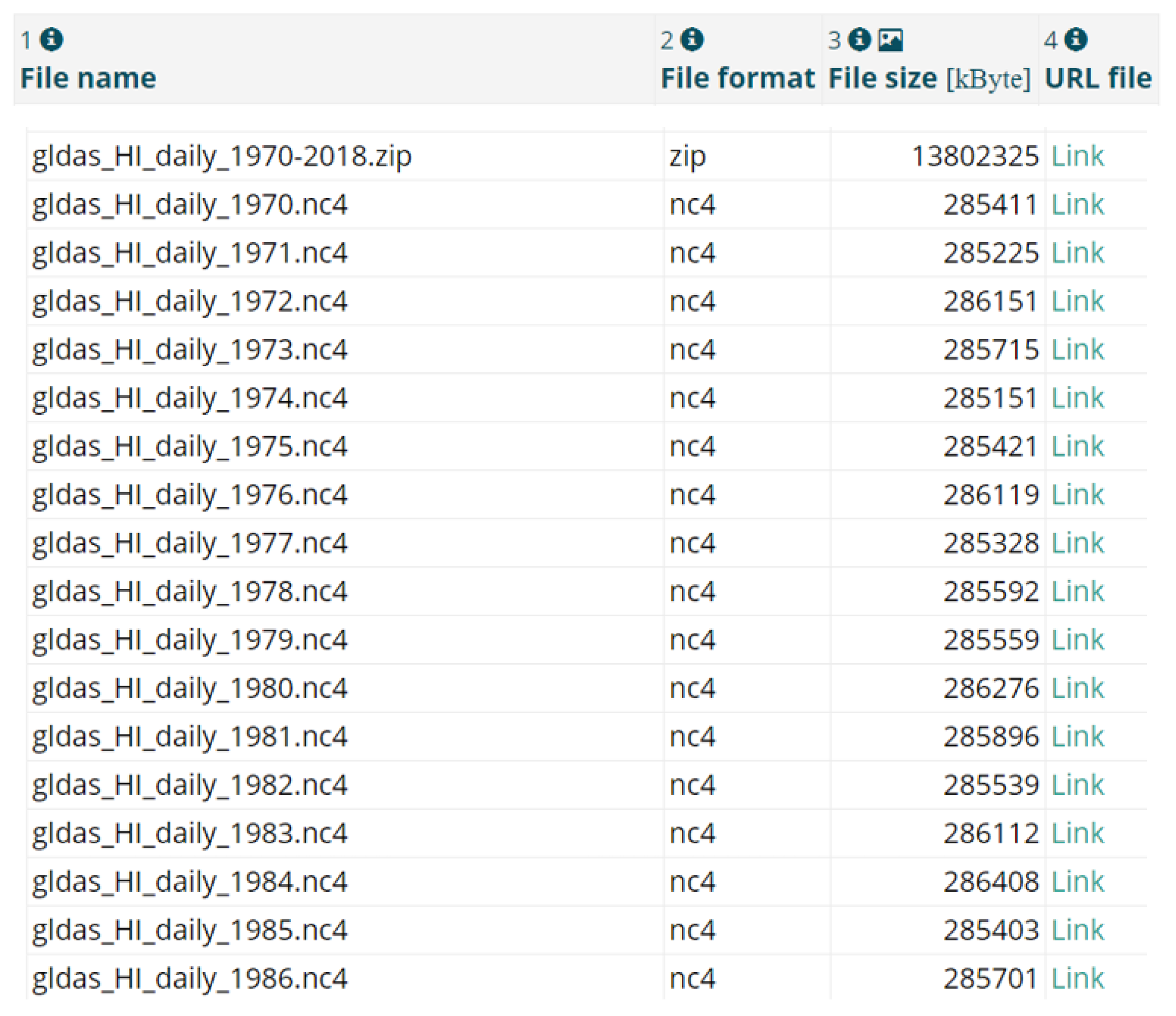
3.1. Data Repository and File Format

All indices in HDI_0p25_1970_2018 (Table 1) are made publicly available in the commonly used scientific Network Common Data Form 4 (NetCDF-4) file format (“.nc4”) on PANGAEA https://doi.org/10.1594/PANGAEA.904282 [83] (Figure 2). The secondary variables (Equations (18)–(21) below) based on GLDAS are available from the author upon request. Both the HDIs and the secondary variables are on daily timescales spanning years 1970–2018. Data for each HDI are bundled as individual annual .nc4 files, as well as a single .nc4 file containing all 49 years.

VP = (P × Q)/(Q + 0.622)

(18)

SVP = 6.11 × exp[17.625 × T_a/(T_a + 243.04)]

(19)

RH = (VP/SVP) × 100

(20)

VPD = [1 − (RH/100)] × SVP

(21)

One of the advantages of .nc4 file format is data compression. All .nc4 files are compressed using CDO command: cdo -z zip_5 copy input.nc4 compressed.nc4, thus reducing file size by a factor of ≈3. The size of the compressed individual annual files varies between 280 and 300 megabytes (MB) depending on the HDI, with the combined time-series (49 years) file ≈14 gigabyte (GB) in size. The total size of all 10 HDIs are ≈140 GB. The files follow the naming convention “gldas_HDI_daily_year.nc4”, wherein “HDI” is the abbreviation of the index (Table 1), and “year” the year over which the HDIs are computed on daily timesteps. Some of the indices use more than one definition for computation in literature (e.g., ABM and NOAA, for AT in Table 1). These abbreviations are also included in the filenames.

3.2. Data Grid, Spatial Coverage, Resolution, and Projection

The spatial extent of GLDAS covers all land north of 60°S latitude and does not include data at or near water bodies. Such grid cells where the required GLDAS data are not available for computing the HDIs are identified by missing values “1.e+20f”. The spatial grid ranges from −59.875 to 89.875 latitude and −179.875 to 179.875 longitude at 0.25° resolution (EPSG projection 4326–“+proj=longlat +ellps=WGS84+datum=WGS84+no_defs”). Consequently, the HDIs (as well as the secondary variables) in HDI_0p25_1970_2018 are also computed over the corresponding 1440 (longitude) × 600 (latitude) grid cells spanning 90° N–60° S, at the same 0.25° gridded resolution, with the land grid-cells in the proximity of water bodies reporting missing values.

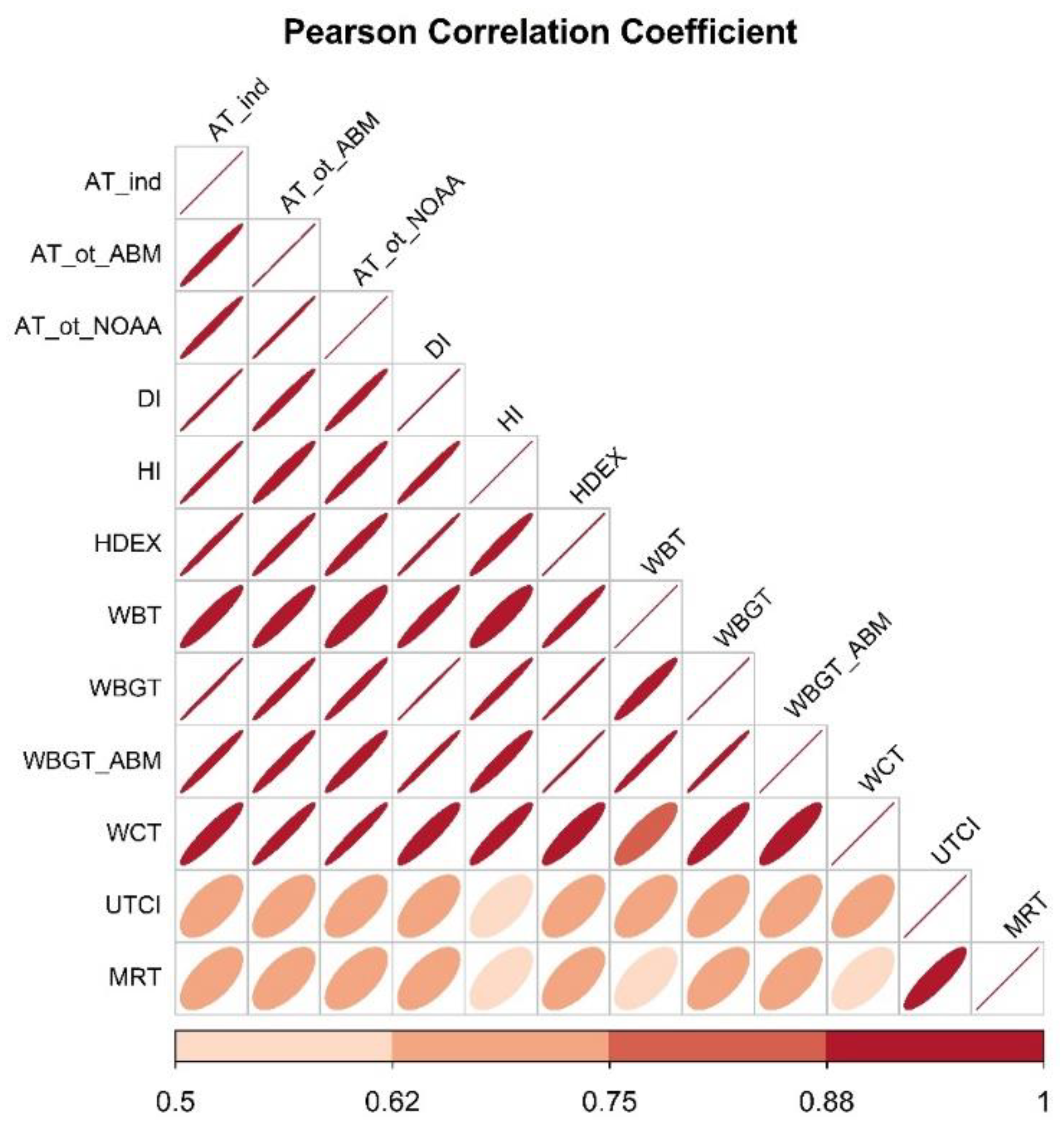
3.3. Technical Validation

GLDAS has been comprehensively evaluated using different regional/global reference datasets in earlier studies, such as [84] who compare the GLDAS daily surface air temperature at 0.25° gridded resolution with two reference datasets: (a) Daymet data (2002 and 2010) for the conterminous U.S. at 1-km gridded resolution, and (b) global meteorological observations (2000) from the Global Historical Climatology Network (GHCN) [85]. A few notable examples of earlier studies that have incorporated GLDAS data include (i) high-resolution global-gridded datasets of climate extreme indices [86] and cooling/heating degree-days [87], and (ii) climate impacts assessment in energy sector [14,15]. Further details on studies implementing GLDAS are available on [88].

Given the lack of any other publicly available regional or global historical dataset incorporating the HDIs discussed in this article, a direct comparison of the indices in HDI_0p25_1970_2018 either at point-specific locations or at aggregated gridded scale is currently not feasible. The HDIs are instead compared with the two HDIs UTCI and MRT recently made available by the Copernicus CDS [36,37]. Maps in Figure 3 below show the heat-stress over western and central Europe, well documented for the 2003 heatwave. For the purpose of comparison, HDIs for July 27, 2003 are shown using a common color legend scale. Focusing on south-western Europe, majority of HDIs capture the unprecedented heat wave over southern-France and most of Spain in particular, with the two HDIs from ERA5-HEAT dataset showing a similar pattern.

It is worth emphasizing that the category of heat stress varies by HDI, and so a visual comparison of the values across HDIs (Figure 3) is not the most appropriate way of comparing the heat stress represented across the HDIs. To facilitate better comparison and evaluate a broader agreement in the spatial patterns across the HDIs, Figure 4 below shows the “Pearson” correlation computed using the spatial maps in Figure 3. It is interesting to note the high correlations (0.88–0.99) across the 10 HDIs in this study. It is also worth noting that although MRT is a component used in the computation of UTCI [36], the correlation between the two is only marginally higher (0.88) compared to the moderately high correlations between each of the 10 HDIs and UTCI/MRT (0.60–0.66). Readers are cautioned though that the spatial correlations shown in Figure 4 are only representative of a particular point in time, for a selective spatial domain (western and central Europe), and during a selective heat wave episode. A detailed comparison and analysis of each HDI during both average and extreme thermal comfort conditions are left for research in future.

4. Discussion

Driven largely by the demands of climate health impact modelers, public health experts, and health-care infrastructure planners, a new historical high spatiotemporal resolution global gridded dataset of multiple HDIs constructed using various meteorological parameters is presented in this study. The dataset is aimed to address a common recurring pitfall faced by the research community; that of freely available, ready to use comprehensive set of quality controlled HDIs for rapid implementation in studies focusing on human health under varying degree of environmental thermal exposure. Nevertheless, certain limitations of the dataset, along with the key features, scope of application, and examples of usage are important to be highlighted.

4.1. Data Limitations

4.1.1. Data Limitations in HDI_0p25_1970_2018 Emanating from GLDAS

The use of GLDAS variables for assembling HDIs in this study was motivated for reasons discussed in Section 2.1 “Source of Meteorological Variables”. Whenever possible, applications of HDIs (especially in impacts assessment) should incorporate input variables from different underlying data products to account for parameter and input data source uncertainty. For instance, as highlighted in [86,87], certain known limitations of GLDAS data, such as larger uncertainty in the surface air temperature estimates over high mountainous areas are well documented in literature [84]. Users of the GLDAS-derived data products are therefore recommended to pay attention to the data caveats.

Moreover, as highlighted earlier, the grid cells in the proximity of water bodies do not report HDIs because of missing data in GLDAS. For studies focusing on point locations or regions smaller than ≈27 × 27 km² in the vicinity of water bodies (such as lakes and rivers, especially in densely populated areas near coastal region), users can be marginally restricted in the usage of the dataset. Such instances in HDI_0p25_1970_2018 are likely to be minimal because the criteria to assign the grid cell as land or water in GLDAS ver-2 data are based on a very high-resolution land-water mask (see further details in Appendix A Figure A1 and the associated discussion). One work around is to fill such gaps using an appropriate interpolation technique available in R, CDO, etc. (e.g., bilinear, near neighbor, inverse-distance mapping).

Another shortcoming of the existing dataset is the lack of uncertainty estimates in the HDIs. Unlike ECMWF ERA5 reanalysis data, GLDAS does not provide ensemble members and so parameter uncertainties of the input meteorological fields are not accounted for in the computation of HDIs. The users of HDI_0p25_1970_2018 are thus reminded that the HDIs should be considered as representative of the ensemble mean of GLDAS realization, and not the spread. Nonetheless, the computation of HDIs on each ensemble member would be a daunting task requiring higher computational and storage facilities.

4.1.2. Limitations in the Current Set of HDIs Presented in This Article

A large number of HDIs derived using numerical and/or experimental approaches, applicable in both indoor and outdoor environments have been documented since the early 1900s (see Table 3 in Epstein and Moran [21]; and Table 1 in Havenith and Fiala [32] for a comprehensive historical summary of the HDIs). As emphasized by Havenith [93] and Pappenberger et al. [94], other meteorological factors such as short- and long-wave radiant fluxes also need to be considered when correctly determining thermal stress.

The current set of HDIs discussed in this article do not directly account for other atmospheric variables such as SR and cloud cover. More complex indices such as the Moran’s Environment Stress Index (ESI, °C) [71], Perceived Temperature (PT, °C) [25] and UTCI (°C) [95,96], are left for work in future.

While the HDIs presented in this article are largely defined using the standard methods in the literature, a few of them use alternative definitions or approximations. For instance, the two versions of WBGT (Equations (10) and (11)) included in the current set of HDIs are simplified versions of the WBGT not accounting for the black globe temperature (T_g) (see [21,50,70] for extensive discussions on different formulations of WBGT employing T_g). Similarly, whereas the AT included in the dataset does not account for SR (see [32] for a variation of AT_{ot_ABM} introduced in Equation (2)), the WCT based on Sipel and Passel (Equation (17)) excludes both SR and humidity [53].

None of the HDIs account for the heat balance mechanisms of the human body. Such HDIs (e.g., UTCI) require a number of parameters based on physiological models [50]. The present dataset is therefore restrictive to “direct indices” [21], i.e., those accounting for only direct measurements of environmental variables proxying heat strain in lieu of a physiologically thermal balance approach.

Finally, all HDIs discussed in this article fall under the category of an “absolute HDI”. A detailed description of a “relative HDI” is outside the scope of this article and readers are referred to [69] for a detailed comparison between an absolute and a relative HDI, and development of one such index known as “WSI”. The difference between the two in a nutshell emanates from the region-specific scope of application. Put simply, HI with a value of 34 °C both in Texas (U.S.) and Berlin (Germany) could have different implications on human activities. Depending on the scope of study, users are reminded to examine alternative formulations and pay attention to limitations of the HDIs in their current form.

4.2. Key Features of the Dataset

Minimum, maximum, or average ambient temperature at sub-daily and daily timescales are often the only variables used in the definition of a majority of thermal indices (see [86,97,98] for further details on the heat wave indices defined using various temperature thresholds). However, such thermal indices when not accounting for other important factors that play a pivotal role (e.g., RH and W), may not provide a realistic assessment of comfort [42]. This is especially more pertinent in coastal regions where large diurnal variations in RH are usually observed. Despite some limitations highlighted earlier, the “direct” HDIs assembled here using a combination of T_a, W, and variants of RH are useful in their ability to encompass the perceived thermal effects into a single number, and therefore interpretable as the more commonly used T_a. To this date, HDI_0p25_1970_2018 spanning 49 years is the only high-resolution global gridded historical dataset of a broad suite of HDIs available to the research community. Along with the subsidiary variables, the dataset offers users with immense flexibility in spatiotemporal aggregation of individual indices (see example shown in Section 4.4).

4.3. Scope of Application

The indices in HDI_0p25_1970_2018 are aimed towards the research community and policy makers focusing largely on but not limited to (a) the impacts of climate change on health and energy sectors; (b) energy as a form of thermal adaptation (e.g., air conditioning) in discomfort environments that are not necessarily work environments; (c) historical trends and patterns in OHS. Bio-meteorological conditions can however show significant intra-day fluctuations, especially in the temperate climate zones. The specific values of the HDIs presented here are representative of the average daily thermal discomfort levels. The daily timescales of the HDIs in this study may therefore make the data less suitable for attribution of health outcomes on intra-day extremes of thermal discomfort levels. For such applications, users are recommended to explore other datasets at sub-daily timescales (e.g., ERA5-HEAT [36]).

Since the individual HDIs in HDI_0p25_1970_2018 are essentially a large panel data (time series of a multiple geo-referenced locations), the dataset can find wider application in both detection/attribution studies (e.g., teleconnections patterns [78,99], amplification or trends under historical warming patterns [99,100]), as well in statistical/econometric analysis incorporating daily mortality and/or morbidity data (e.g., labor productivity under climate change—see [101] and references therein).

Assembled at a high spatiotemporal resolution, HI_0p25_1970_2018 allows users to aggregate the indices both at spatial (such as administrative levels, national boundaries), as well as temporal scales (such as months, seasons). It is worth emphasizing once again that the HDIs (Table 1), are assembled at the same spatiotemporal resolution (daily, 0.25°) as the near-surface daily averaged secondary variables outlined in Table 2. Each HDI therefore represents the estimated mean daily historical human discomfort conditions averaged over the 0.25° grid boxes (≈27 × 27 km at the equator).

A primary aim to assemble the HDIs uniformly over time and space, and across all global land grid-cells at high spatial resolution, motivated the choice of meteorological variables from a quality-controlled reanalysis data product in this study. Consequently, utilizing station point data (e.g., ECA&D [102]) or other gridded data products from either national (e.g., Brazil [103], India [104]), regional (e.g., E-OBS [105], ClimateNA [106]), or global meteorological data sources (e.g., GHCN [85]) at coarser resolutions were not considered in the preparation of HDIs presented in this article. Nonetheless, depending on the broader spatiotemporal application of the HDIs, researchers are encouraged to use other data sources in conjunction with the GLDAS based HDI_0p25_1970_2018 dataset presented here. The code utilized in this article for the preparation of HDIs is available upon request for rapid portability to other data sources.

Table 3 summarizes the descriptive categories of thermal comfort levels across selective HDIs used in this article. It must be highlighted that while the HDIs at a particular location may have been recorded within their operational thresholds, certain HDIs by definition are more suited for particular climate zones than the others (e.g., DI which considers temperatures ranging from 24 to 27 °C as uncomfortable is intuitively more suitable for midlatitude countries with cooler climate compared to tropics).

In the context of a historical dataset presented here, the global coverage of the HDI_0p25_1970_2018 offers users a unique opportunity to examine spatiotemporal variability using sophisticated techniques, such as the space–time perspective approach using rotated Empirical Orthogonal Functions (EOFs) (see Chen and Tung [107] for methodology adopted using rotated EOFs to examine global-mean surface temperature variability and associated large-scale teleconnections with El Nino-Southern Oscillation Index among others). HDI_0p25_1970_2018 can also facilitate examining the impacts of climate change on heat stress.

Moreover, the impact of extreme human discomfort levels could be more detrimental in densely congested regions, in particular to the socio-economically vulnerable people having little or no availability to counter-acting adaptation measures (e.g., usage of air-conditioning, see [14]). Accounting for population exposure across the extreme ranges of the HDIs over regional boundaries for instance (i.e., population weighted HDIs), can facilitate demographic stratification of sectoral impacts.

It is important to emphasize that while the HDIs are primarily designed for climate-health experts to gauge exposure risk to humans under different thermal environments, the spill-over effects are not necessarily limited to the health sector. For instance, a recent report by the International Labor Organization (ILO) [108] highlights heat related morbidity and mortality can have wider implications for labor productivity, economy, and social conditions. Similarly, the energy sector could also have implications with subsequent escalations in energy demands for maintaining thermal comfort levels, and shift in investments towards environmentally friendly modes of cooling.

4.4. Tools and Recommended Ways to Use the Dataset

NetCDF-4 facilitates data compression, portability, scalability, and is the de facto file format in the climate science community. It is compatible with a number of open-access software environments and desktop Geographic Information System (GIS) tools for generating quick plots, and for exploratory and geo-spatial data analysis. A non-exhaustive list of such freely available tools includes: (i) Panoply [109], and (ii) NCview [110] for generating quick plots and exploring .nc4 file data structure; while (iii) R [111], and (iv) Python [112] are recommended for data manipulation, exploratory and geospatial analysis, statistical/econometric modelling; (v) QGIS [113] and (vi) GRASS GIS [114] are recommended for users comfortable with graphical user interface (GUI) based environments.

Handling high resolution global gridded netCDF files can be computationally and memory intensive on standard machines with ≈4 GB of RAM. Whenever work scope requires focusing on smaller spatial subset of data (e.g., summer months—June to September—over a spatial domain covering China), users are first recommended to subset the .nc4 files prior reading them in certain software environments (e.g., R) where memory usage can be high. For such rapid data manipulation (spatiotemporal extraction etc.), as well as for exploring the variables, dimensions, units, attributes, etc., within the .nc4 file structure, users are recommended to employ command line routines made available in NCO and/or CDO. For e.g., NCO command “ncdump-h filename.nc4” or its equivalent CDO command “cdo sinfo filename.nc4” would allow a user to print the entire three-dimensional file structure. Readers are guided to the comprehensive user guides of NCO [61] and CDO [62] for reference commands.

Made available at daily timesteps, the HDIs are not recommended to be aggregated to other temporal scales (as highlighted in Section 4.3), such as weekly, monthly, seasonal, and annual timescales. While aggregation can be rapidly undertaken using NCO/CDO commands (as well as R, Python, etc.), multi-year daily statistics, and spatial aggregation to defined polygon boundaries (e.g., regions, provinces etc., using appropriate shape files) are instead more recommended ways when handling the HDIs. For instance, the native 0.25° gridded resolution can be re-gridded (interpolated) to either finer or coarser gridded resolution (e.g., 0.15° or 0.5°) using remapping techniques available in various geo-spatial tools, such as the CDO [62] remapping functions (e.g., “remapbil”) or R raster [89] package. Users are cautioned though of a possible aggregation/disaggregation bias that may result because of remapping to different spatial scales.

For illustration, a sample R code (“HDI_sample_script.R”) is provided in Supplementary Material to facilitate spatiotemporal sub-setting and aggregation of the DI over regional boundaries of Italy. The script does the following:

(i)

Downloads “gldas_DI_daily_2003.nc4” from the PANGAEA repository within R environment (a direct download from the repository is another alternative);

(ii)

Using the downloaded global gridded daily data, annual and monthly averages of DI for year 2003 are computed at each grid-cell for the full global domain (although this is for illustration purpose only as temporal aggregation is not recommended, discussed above);

(iii)

Utilizing a country shape file for Italy (Admin 1 level, regional boundaries), the grid-cell level monthly averages computed in step (ii) are cropped to the national boundary of Italy;

(iv)

The monthly grid-cells extracted in step (iii) are aggregated over the Italian regional boundaries, to produce regional level monthly values of DI for 2003;

(v)

Sample plot (map) of the aggregated index obtained from step (iv) is saved as a “.png” file;

(vi)

The aggregated data index from steps (iii) and (iv) are saved as output in three different file formats (a) Ascii, “.csv”, (b) Netcdf, “.nc”, and (c) GeoTiff “.tiff”.

5. Work Planned for Future

The indices in HDI_0p25_1970_2018 are intended to be updated post-2018 years, subject to the availability of the required GLDAS raw meteorological variables in the coming years. The updated netCDF files will be made available to users on the same data repository, and users are encouraged to consult the author for any going updates prior accessing the existing data from the repository. In addition, spatiotemporal aggregation of the current set of HDIs for rapid implementation in impacts analyses, and development of a broader set of HDIs not included in this article are also envisaged in the near future.

While netCDF is more common and popular with the climate modeling community, and also facilities easier data storage and transfer, risk and impact assessment modelers often prefer data in easier and ready to use formats (e.g., “.csv”, “.tiff”) for implementation in their geo-spatial and statistical/econometric frameworks. Such data in other commonly used formats (e.g., ASCII, GeoTIFF) require additional data transformation and storage from the existing .nc4 files provided in the repository. In addition, users may also prefer an option to download selective years and/or regions instead of the heavier netCDF files.

To facilitate such a choice of downloadable data format, as well as user-defined spatiotemporal sub-setting of the HDIs to smaller domains, a graphical user interface (GUI) tool is planned for the benefit of the wider user community. Once implemented, the webpage URL of the tool will be indicated on the current PANGAEA repository.

6. Code Availability

All codes for assembling the HDIs (Table 1) and the associated secondary variables (Table 2), are available from the author upon request. The code for data generation of HDIs and secondary variables includes a combination of CDO [62] (ver 1.9.0) and NCO [61] (ver 4.3.4) commands written in Unix bash (shell) scripts, customized to run in a parallel super-computing infrastructure. Sample R code (“HDI_sample_script.R”) discussed in Section 4.4, is provided for illustration in supplementary material. The code written in open source R [111] software (version 3.5.0—“Joy in Playing”), downloads, reads, analyses, transforms, plots, and saves the output of a sample HDI. All codes used in this study are developed on x86_64 Linux CentOS 6.6 software architecture but can be adapted to Windows as well as MacOSX.

References

1. Tomczyk, A.M.; Bednorz, E. Heat waves in Central Europe and tropospheric anomalies of temperature and geopotential heights. Int. J. Climatol. 2019, 39, 4189–4205. [Google Scholar] [CrossRef]
2. Tomczyk, A.M.; Bednorz, E.; Matzarakis, A. Human-biometeorological conditions during heat waves in Poland. Int. J. Climatol. 2020, 1–13. [Google Scholar] [CrossRef]
3. Satyanarayana, G.C.; Rao, D.V.B. Phenology of heat waves over India. Atmos. Res. 2020, 245, 105078. [Google Scholar] [CrossRef]
4. Krzyżewska, A.; Wereski, S.; Demczuk, P. Biometeorological conditions during an extreme heatwave event in Poland in August 2015. Weather 2020, 75, 183–189. [Google Scholar] [CrossRef]
5. Hoy, A.; Hänsel, S.; Maugeri, M. An endless summer: 2018 heat episodes in Europe in the context of secular temperature variability and change. Int. J. Climatol. 2020, 1–22. [Google Scholar] [CrossRef] [Green Version]
6. Loughran, T.F.; Perkins-Kirkpatrick, S.E.; Alexander, L. V Understanding the spatio-temporal influence of climate variability on Australian heatwaves. Int. J. Climatol. 2017, 37, 3963–3975. [Google Scholar] [CrossRef]
7. Kjellstrom, T. Climate change, heat exposure and labour productivity. Epidemiology 2000, 11, S144. [Google Scholar]
8. Kjellstrom, T.; Holmer, I.; Lemke, B. Workplace heat stress, health and productivity—An increasing challenge for low and middle-income countries during climate change. Glob. Health Action 2009, 2. [Google Scholar] [CrossRef]
9. Kjellstrom, T.; Briggs, D.; Freyberg, C.; Lemke, B.; Otto, M.; Hyatt, O. Heat, Human Performance, and Occupational Health: A Key Issue for the Assessment of Global Climate Change Impacts. Annu. Rev. Public Health 2016, 37, 97–112. [Google Scholar] [CrossRef] [Green Version]
10. Opitz-Stapleton, S.; Sabbag, L.; Hawley, K.; Tran, P.; Hoang, L.; Nguyen, P.H. Heat index trends and climate change implications for occupational heat exposure in Da Nang, Vietnam. Clim. Serv. 2016, 2–3, 41–51. [Google Scholar] [CrossRef] [Green Version]
11. Orlov, A.; Sillmann, J.; Aaheim, A.; Aunan, K.; de Bruin, K. Economic Losses of Heat-Induced Reductions in Outdoor Worker Productivity: A Case Study of Europe. Econ. Disasters Clim. Chang. 2019, 3, 191–201. [Google Scholar] [CrossRef]
12. Mora, C.; Dousset, B.; Caldwell, I.R.; Powell, F.E.; Geronimo, R.C.; Bielecki, C.R.; Counsell, C.W.W.; Dietrich, B.S.; Johnston, E.T.; Louis, L.V.; et al. Global risk of deadly heat. Nat. Clim. Chang. 2017, 7, 501–506. [Google Scholar] [CrossRef]
13. Matthews, T. Humid heat and climate change. Prog. Phys. Geogr. 2018, 42, 391–405. [Google Scholar] [CrossRef] [Green Version]
14. De Cian, E.; Pavanello, F.; Randazzo, T.; Mistry, M.; Davide, M. Households’ adaptation in a warming climate. Air conditioning and thermal insulation choices. Environ. Sci. Policy 2019, 100, 136–157. [Google Scholar] [CrossRef]
15. De Cian, E.; Sue Wing, I. Global Energy Consumption in a Warming Climate. Environ. Resour. Econ. 2019, 72, 365–410. [Google Scholar] [CrossRef]
16. Van Ruijven, B.J.; De Cian, E.; Sue Wing, I. Amplification of future energy demand growth due to climate change. Nat. Commun. 2019, 10, 1–12. [Google Scholar] [CrossRef] [Green Version]
17. Wong, H.T.; Lai, P.C. Weather inference and daily demand for emergency ambulance services. Emerg. Med. J. 2012, 29, 60–64. [Google Scholar] [CrossRef]
18. Turner, L.; Connell, D.; Tong, S. The Effect of Heat Waves on Ambulance Attendances in Brisbane, Australia. Prehosp. Disaster Med. 2013, 28, 1–6. [Google Scholar] [CrossRef] [Green Version]
19. Gao, C.; Kuklane, K.; Östergren, P.-O.; Kjellstrom, T. Occupational heat stress assessment and protective strategies in the context of climate change. Int. J. Biometeorol. 2018, 62, 359–371. [Google Scholar] [CrossRef]
20. Kjellstrom, T.; Freyberg, C.; Lemke, B.; Otto, M.; Briggs, D. Estimating population heat exposure and impacts on working people in conjunction with climate change. Int. J. Biometeorol. 2018, 62, 291–306. [Google Scholar] [CrossRef]
21. Epstein, Y.; Moran, D.S. Thermal Comfort and the Heat Stress Indices. Ind. Health 2006, 44, 388–398. [Google Scholar] [CrossRef] [PubMed] [Green Version]
22. Parsons, K. Human Thermal Environments: The Effects of Hot, Moderate, and Cold Environments on Human Health, Comfort, and Performance, 3rd ed.; CRC Press, Inc.: Boca Raton, FL, USA, 2014; ISBN 146659599X, 9781466595996. [Google Scholar]
23. Health and Safety Executive (HSE) Six Factors of Thermal Discomfort. Available online: https://www.hse.gov.uk/temperature/thermal/factors.htm (accessed on 10 May 2020).
24. Rothfusz, L. The Heat Index “Equation” (or, More Than You Ever Wanted to Know About Heat Index). Available online: https://www.weather.gov/media/ffc/ta_htindx.pdf (accessed on 20 March 2020).
25. Jendritzky, G.; Staiger, H.; Bucher, K.; Graetz, A.; Laschewski, G. The Perceived Temperature: The Method of the Deutscher Wetterdienst for the Assessment of Cold Stress and Heat Load for the Human Body. Int. J. Biometeorol. 2012, 56, 165–176. [Google Scholar]
26. Stull, R. Wet-Bulb Temperature from Relative Humidity and Air Temperature. J. Appl. Meteorol. Climatol. 2011, 50, 2267–2269. [Google Scholar] [CrossRef] [Green Version]
27. Tetens, O. Uber cinige meteorologische Begriffe. Z. Geophys. 1930, 6, 297–309. [Google Scholar]
28. Thom, E.C. The Discomfort Index. Weatherwise 1959, 12, 57–61. [Google Scholar] [CrossRef]
29. Masterton, J.M.; Richardson, F.A. Humidex: A Method of Quantifying Human Discomfort Due to Excessive Heat and Humidity; CLI 1-79; Environment Canada, Atmospheric Environment: Downsview, ON, USA, 1979; p. 45.
30. Buzan, J.R.; Oleson, K.; Huber, M. Implementation and comparison of a suite of heat stress metrics within the Community Land Model version 4.5. Geosci. Model Dev. 2015, 8, 151–170. [Google Scholar] [CrossRef] [Green Version]
31. De Lima, C.Z.; Buzan, J.R.; Hertel, T.W.; Moore, F.C.; Baldos, U.L.C. Consequences of heat stress on agricultural workers dominates crop impacts of climate change. In Proceedings of the 22th Annual Conference on Global Economic Analysis GTAP, Warsaw, Poland, 19–21 June 2019. [Google Scholar]
32. Havenith, G.; Fiala, D. Thermal indices and thermophysiological modeling for heat stress. Compr. Physiol. 2016, 6, 255–302. [Google Scholar]
33. Streinu-Cercel, A.; Costoiu, S.M.M.; Streinu-Cercel, A.; Mârza, M. Models for the indices of thermal comfort. J. Med. Life 2008, 1, 148–156. [Google Scholar]
34. Davis, R.E.; Knight, D.; Hondula, D.; Knappenberger, P.C. A comparison of biometeorological comfort indices and human mortality during heat waves in the United States. In Proceedings of the 17th Symposium on Boundary Layers and Turbulence, 27th Conference on Agricultural and Forest Meteorology, 17th Conference on Biometeorology and Aerobiology, San Diego, CA, USA, 21–25 May 2006. [Google Scholar]
35. Quayle, R.; Doehring, F. Heat Stress. Weatherwise 1981, 34, 120–124. [Google Scholar] [CrossRef]
36. Di Napoli, C.; Barnard, C.; Prudhomme, C.; Cloke, H.L.; Pappenberger, F. ERA5-HEAT: A global gridded historical dataset of human thermal comfort indices from climate reanalysis. Geosci. Data J. 2020, 1–9. [Google Scholar] [CrossRef]
37. Copernicus Climate Data Store. Available online: https://cds.climate.copernicus.eu/cdsapp#!/dataset/derived-utci-historical?tab=overview (accessed on 27 July 2020).
38. Steadman, R.G. The Assessment of Sultriness. Part I: A Temperature-Humidity Index Based on Human Physiology and Clothing Science. Appl. Meteorol. 1979, 18, 861–873. [Google Scholar] [CrossRef] [Green Version]
39. Steadman, R.G. A Universal Scale of Apparent Temperature. Clim. Appl. Meteorol. 1984, 23, 1674–1687. [Google Scholar] [CrossRef]
40. Steadman, R.G. Norms of apparent temperature in Australia. Aust. Meteorol. Oceanogr. 1994, 43, 1–16. [Google Scholar]
41. Krstić, G. Apparent temperature and air pollution vs. elderly population mortality in Metro Vancouver. PLoS ONE 2011, 6, e25101. [Google Scholar] [CrossRef] [Green Version]
42. Mohan, M.; Gupta, A.; Bhati, S. A Modified Approach to Analyze Thermal Comfort Classification. Atmos. Clim. Sci. 2013, 4, 7–19. [Google Scholar] [CrossRef] [Green Version]
43. Schoen, C. A New Empirical Model of the Temperature–Humidity Index. J. Appl. Meteorol. 2005, 44, 1413–1420. [Google Scholar] [CrossRef]
44. Dahl, K.; Licker, R.; Abatzoglou, J.T.; Declet-Barreto, J. Increased frequency of and population exposure to extreme heat index days in the United States during the 21st century. Environ. Res. Commun. 2019, 1, 075002. [Google Scholar] [CrossRef]
45. Russo, S.; Sillmann, J.; Sterl, A. Humid heat waves at different warming levels. Sci. Rep. 2017, 7, 7477. [Google Scholar] [CrossRef]
46. Atalla, T.; Gualdi, S.; Lanza, A. A global degree days database for energy-related applications. Energy 2018, 143, 1048–1055. [Google Scholar] [CrossRef] [Green Version]
47. Haldane, J.S. The Influence of High Air Temperatures: No. 1. J. Hyg. (Lond.) 1905, 5, 494–513. [Google Scholar] [CrossRef] [PubMed]
48. Pal, J.S.; Eltahir, E.A.B. Future temperature in southwest Asia projected to exceed a threshold for human adaptability. Nat. Clim. Chang. 2016, 6, 197–200. [Google Scholar] [CrossRef]
49. Gagge, A.P.; Nishi, Y. Physical indices of the thermal environment. ASHRAE J. 1976, 18, 1. [Google Scholar]
50. Lemke, B.; Kjellstrom, T. Calculating workplace WBGT from meteorological data: A tool for climate change assessment. Ind. Health 2012, 50, 267–278. [Google Scholar] [CrossRef] [Green Version]
51. ABM Wet Bulb Globe Temperature as defined by Australian Bureau of Meteorology. Available online: http://www.bom.gov.au/info/thermal_stress/ (accessed on 2 June 2019).
52. Siple, P.A.; Passel, C.F. Measurements of Dry Atmospheric Cooling in Subfreezing Temperatures. Proc. Am. Philos. Soc. 1945, 89, 177–199. [Google Scholar] [CrossRef]
53. Groen, G. Wind Chill Equivalent Temperature (WCET) Climatology and Scenarios for Schiphol Airport; KNMI Tech. Report; Koninklijk Nederlands Meteorologisch Instituut: De-Bilt, The Netherlands, 2009; p. 18. [Google Scholar]
54. Quayle, R.G.; Steadman, R.G. The Steadman Wind Chill: An Improvement over Present Scales. Weather Forecast. 1998, 13, 1187–1193. [Google Scholar] [CrossRef]
55. Rodell, M.; Houser, P.R.; Jambor, U.; Gottschalck, J.; Mitchell, K.; Meng, C.-J.C.-J.; Arsenault, K.; Cosgrove, B.; Radakovich, J.; Bosilovich, M.; et al. The Global Land Data Assimilation System. Bull. Am. Meteorol. Soc. 2004, 85, 381–394. [Google Scholar] [CrossRef] [Green Version]
56. Kumar, S.V.; Peters-Lidard, C.D.; Tian, Y.; Houser, P.R.; Geiger, J.; Olden, S.; Lighty, L.; Eastman, J.L.; Doty, B.; Dirmeyer, P.; et al. Land information system: An interoperable framework for high resolution land surface modeling. Environ. Model. Softw. 2006, 21, 1402–1415. [Google Scholar] [CrossRef]
57. Peters-Lidard, C.D.; Houser, P.R.; Tian, Y.; Kumar, S.V.; Geiger, J.; Olden, S.; Lighty, L.; Doty, B.; Dirmeyer, P.; Adams, J.; et al. High-performance Earth system modeling with NASA/GSFC’s Land Information System. Innov. Syst. Softw. Eng. 2007, 3, 157–165. [Google Scholar] [CrossRef]
58. Colston, J.M.; Ahmed, T.; Mahopo, C.; Kang, G.; Kosek, M.; de Sousa, F., Jr.; Shrestha, P.S.; Svensen, E.; Turab, A.; Zaitchik, B. Evaluating meteorological data from weather stations, and from satellites and global models for a multi-site epidemiological study. Environ. Res. 2018, 165, 91–109. [Google Scholar] [CrossRef]
59. NASA-GSFC GLDAS Data. Available online: https://disc.gsfc.nasa.gov/datasets/GLDAS_NOAH025_3H_V2.1/summary (accessed on 12 November 2019).
60. NASA-GSFC-DISC GLDAS Data Access. Available online: https://disc.gsfc.nasa.gov/datasets?page=1&project=GLDAS&temporalResolution=3hours&spatialResolution=0.25°x0.25° (accessed on 15 November 2019).
61. Zender, C.S. Analysis of self-describing gridded geoscience data with netCDF Operators (NCO). Environ. Model. Softw. 2008, 23, 1338–1342. [Google Scholar] [CrossRef] [Green Version]
62. Uwe SCHULZWEIDA of Max Planck Institute for Meteorology. Climate Data Operators (CDO) User Guide, Version 1.9.0; Uwe SCHULZWEIDA: Hamburg, Germany, 2018. [Google Scholar]
63. Webb, A. Principles of environmental physics. By J. L. Monteith & M. H. Unsworth. Edward Arnold, Sevenoaks. 2nd edition, 1990. pp. xii + 291. Q. J. R. Meteorol. Soc. 1994, 120, 1700. [Google Scholar]
64. Stull, R.B. Meteorology for Scientists and Engineers, 3rd ed. 2011. Available online: https://www.eoas.ubc.ca/books/Practical_Meteorology/mse3.html (accessed on 12 November 2019).
65. Steadman, R.G. The Assessment of Sultriness. Part II: Effects of Wind, Extra Radiation and Barometric Pressure on Apparent Temperature. J. Appl. Meteorol. 1979, 18, 874–885. [Google Scholar] [CrossRef] [Green Version]
66. Gonzalez, R.R.; Nishi, Y.; Gagge, A.P. Experimental evaluation of standard effective temperature a new biometeorological index of man’s thermal discomfort. Int. J. Biometeorol. 1974, 18, 1–15. [Google Scholar] [CrossRef] [PubMed]
67. Almeida, S.P.; Casimiro, E.; Calheiros, J. Effects of apparent temperature on daily mortality in Lisbon and Oporto, Portugal. Environ. Heal. 2010, 9, 12. [Google Scholar] [CrossRef] [Green Version]
68. Wichmann, J.; Ketzel, M.; Ellermann, T.; Loft, S. Apparent temperature and acute myocardial infarction hospital admissions in Copenhagen, Denmark: A case-crossover study. Environ. Health 2012, 11, 19. [Google Scholar] [CrossRef] [Green Version]
69. Kalkstein, L.S.; Valimont, K.M. An evaluation of summer discomfort in the United States using a relative climatological index. Bull.—Am. Meteorol. Soc. 1986, 67, 842–848. [Google Scholar] [CrossRef]
70. Yaglou, C.P.; Minaed, D. Control of Heat Casualties at Military Training Centers. Arch. Indust. Heal. 1957, 16, 302–316. [Google Scholar]
71. Moran, D.; Pandolf, K.B.; Shapiro, Y.; Heled, Y.; Shani, Y.; Mathew, W.T.; Gonzalez, R. An environmental stress index (ESI) as a substitute for the wet bulb globe temperature (WBGT). J. Therm. Biol. 2001, 26, 427–431. [Google Scholar] [CrossRef]
72. Budd, G.M. Wet-bulb globe temperature (WBGT)-its history and its limitations. J. Sci. Med. Sport 2008, 11, 20–32. [Google Scholar] [CrossRef]
73. Zare, S.; Hasheminejad, N.; Shirvan, H.E.; Hemmatjo, R.; Sarebanzadeh, K.; Ahmadi, S. Comparing Universal Thermal Climate Index (UTCI) with selected thermal indices/environmental parameters during 12 months of the year. Weather Clim. Extrem. 2018, 19, 49–57. [Google Scholar] [CrossRef]
74. Goldie, J.; Alexander, L.; Lewis, S.C.; Sherwood, S. Comparative evaluation of human heat stress indices on selected hospital admissions in Sydney, Australia. Aust. N. Z. J. Public Health 2017, 41, 381–387. [Google Scholar] [CrossRef] [PubMed]
75. Dear, K. Modelling productivity loss from heat stress. Atmosphere 2018, 9, 286. [Google Scholar] [CrossRef] [Green Version]
76. Sohar, E.; Adar, R.; Kaly, J. Comparison of the environmental heat load in various parts of Israel. Bull. Res. Counc. Isr. E 1963, 10, 111–115. [Google Scholar]
77. Sohar, E.; Birenfeld, C.; Shoenfeld, Y.; Shapiro, Y. Description and forecast of summer climate in physiologically significant terms. Int. J. Biometeorol. 1978, 22, 75–81. [Google Scholar] [CrossRef]
78. Almendra, R.; Santana, P.; Vasconcelos, J.; Silva, G.; Gonçalves, F.; Ambrizzi, T. The influence of the winter North Atlantic Oscillation index on hospital admissions through diseases of the circulatory system in Lisbon, Portugal. Int. J. Biometeorol. 2017, 61, 325–333. [Google Scholar] [CrossRef] [Green Version]
79. Osczevski, R.J. The Basis of Wind Chill. Arctic 1995, 48, 372–382. [Google Scholar] [CrossRef] [Green Version]
80. Steadman, R.G. Indices of windchill of clothed persons. J. Appl. Meteorol. 1971, 10, 674–683. [Google Scholar] [CrossRef]
81. LeBlanc, J.; Blais, B.; Barabe, B.; Cote, J. Effects of temperature and wind on facial temperature, heart rate, and sensation. J. Appl. Physiol. 1976, 40, 127–131. [Google Scholar] [CrossRef]
82. Virokannas, H.; Anttonen, H. Thermal responses in the body during snowmobile driving. Arctic Med. Res. 1994, 53 (Suppl. 3), 12–18. [Google Scholar]
83. Mistry, M.N. A High Spatiotemporal Resolution Global Gridded Dataset of Historical (1970–2018) Human Discomfort Indices Based on GLDAS Data. Available online: https://doi.org/10.1594/PANGAEA.904282 (accessed on 14 May 2020).
84. Ji, L.; Senay, G.B.; Verdin, J.P. Evaluation of the Global Land Data Assimilation System (GLDAS) Air Temperature Data Products. J. Hydrometeorol. 2015, 16, 2463–2480. [Google Scholar] [CrossRef]
85. Menne, M.J.; Durre, I.; Vose, R.S.; Gleason, B.E.; Houston, T.G. An Overview of the Global Historical Climatology Network-Daily Database. J. Atmos. Ocean. Technol. 2012, 29, 897–910. [Google Scholar] [CrossRef]
86. Mistry, M.N. A High-Resolution Global Gridded Historical Dataset of Climate Extreme Indices. Data 2019, 4, 41. [Google Scholar] [CrossRef] [Green Version]
87. Mistry, M.N. Historical global gridded degree-days: A high-spatial resolution database of CDD and HDD. Geosci. Data J. 2019, 6, 214–221. [Google Scholar] [CrossRef] [Green Version]
88. GLDAS Previous Studies. Available online: https://ldas.gsfc.nasa.gov/gldas/publications (accessed on 29 May 2020).
89. Hijmans, R.J.; van Etten, J. Raster: Geographic Data Analysis and Modeling. Available online: https://cran.r-project.org/package=raster (accessed on 15 December 2019).
90. Pebesma, E.J.; Bivand, R.S. Classes and methods for spatial data in {R}. R News 2005, 5, 9–13. [Google Scholar]
91. Bivand, R.S.; Pebesma, E.; Gomez-Rubio, V. Applied spatial data analysis with {R}, 2nd ed.; Springer: New York, NY, USA, 2013. [Google Scholar]
92. Wei, T.; Simko, V. R package “corrplot”: Visualization of a Correlation Matrix. Available online: https://github.com/taiyun/corrplot (accessed on 26 July 2020).
93. Havenith, G. Individualized model of human thermoregulation for the simulation of heat stress response. J. Appl. Physiol. 2001, 90, 1943–1954. [Google Scholar] [CrossRef]
94. Pappenberger, F.; Jendritzky, G.; Staiger, H.; Dutra, E.; Di Giuseppe, F.; Richardson, D.S.; Cloke, H.L. Global forecasting of thermal health hazards: The skill of probabilistic predictions of the Universal Thermal Climate Index (UTCI). Int. J. Biometeorol. 2015, 59, 311–323. [Google Scholar] [CrossRef] [Green Version]
95. Fiala, D.; Havenith, G.; Bröde, P.; Kampmann, B.; Jendritzky, G. UTCI-Fiala multi-node model of human heat transfer and temperature regulation. Int. J. Biometeorol. 2012, 56, 429–441. [Google Scholar] [CrossRef] [Green Version]
96. Bröde, P.; Fiala, D.; Błażejczyk, K.; Holmér, I.; Jendritzky, G.; Kampmann, B.; Tinz, B.; Havenith, G. Deriving the operational procedure for the Universal Thermal Climate Index (UTCI). Int. J. Biometeorol. 2012, 56, 481–494. [Google Scholar] [CrossRef] [Green Version]
97. Alexander, L.; Herold, N. ClimPACT2 Indices and Software (R Software Package). Available online: https://htmlpreview.github.io/?https://raw.githubusercontent.com/ARCCSS-extremes/climpact2/master/user_guide/ClimPACT2_user_guide.htm (accessed on 11 December 2019).
98. Perkins, S.E.; Alexander, L. V On the Measurement of Heat Waves. J. Clim. 2013, 26, 4500–4517. [Google Scholar] [CrossRef]
99. Dobrinescu, A.; Busuioc, A.; Birsan, M.-V.; Dumitrescu, A.; Orzan, A. Changes in thermal discomfort indices in Romania and their connections with large-scale mechanisms. Clim. Res. 2015, 64, 213–226. [Google Scholar] [CrossRef]
100. Talukdar, M.S.; Hossen, M.; Baten, A. Trends of Outdoor Thermal Discomfort in Mymensingh: An Application of Thoms’ Discomfort index. J. Environ. Sci. Nat. Resour. 2018, 10, 151–156. [Google Scholar] [CrossRef] [Green Version]
101. Day, E.; Fankhauser, S.; Kingsmill, N.; Costa, H.; Mavrogianni, A. Upholding labour productivity under climate change: An assessment of adaptation options. Clim. Policy 2019, 19, 367–385. [Google Scholar] [CrossRef]
102. Klok, E.J.; Klein Tank, A.M.G. Updated and extended European dataset of daily climate observations. Int. J. Climatol. 2009, 29, 1182–1191. [Google Scholar] [CrossRef]
103. Xavier, A.C.; King, C.W.; Scanlon, B.R. Daily gridded meteorological variables in Brazil (1980–2013). Int. J. Climatol. 2016, 36, 2644–2659. [Google Scholar] [CrossRef] [Green Version]
104. Srivastava, A.K.; Rajeevan, M.; Kshirsagar, S.R. Development of a high resolution daily gridded temperature data set (1969–2005) for the Indian region. Atmos. Sci. Lett. 2009, 10, 249–254. [Google Scholar] [CrossRef]
105. Cornes, R.C.; van der Schrier, G.; van den Besselaar, E.J.M.; Jones, P.D. An Ensemble Version of the E-OBS Temperature and Precipitation Data Sets. J. Geophys. Res. Atmos. 2018, 123, 9391–9409. [Google Scholar] [CrossRef] [Green Version]
106. Wang, T.; Hamann, A.; Spittlehouse, D.; Carroll, C. Locally downscaled and spatially customizable climate data for historical and future periods for North America. PLoS ONE 2016, 11, e0156720. [Google Scholar] [CrossRef] [PubMed]
107. Chen, X.; Tung, K.-K. Global-mean surface temperature variability: Space–time perspective from rotated EOFs. Clim. Dyn. 2018, 51, 1719–1732. [Google Scholar] [CrossRef] [Green Version]
108. ILO Working On a Warmer Planet: The Impact of Heat Stress on Labour Productivity and Decent Work. Available online: https://www.ilo.org/wcmsp5/groups/public/---dgreports/---dcomm/---publ/documents/publication/wcms_711919.pdf (accessed on 27 April 2020).
109. NASA GISS Panoply Software. Available online: https://www.giss.nasa.gov/tools/panoply/ (accessed on 12 January 2020).
110. Pierce, D.W. Ncview Software Scripps Institution of Oceanography. Available online: http://meteora.ucsd.edu/~pierce/ncview_home_page.html (accessed on 11 January 2020).
111. R Core Team R: A Language and Environment for Statistical Computing. Available online: https://www.r-project.org/ (accessed on 21 October 2019).
112. Van Rossum, G.; Drake, F.L. Python 3 Reference Manual; CreateSpace: Scotts Valley, CA, USA, 2009; ISBN 1441412697. [Google Scholar]
113. QGIS.org QGIS Geographic Information System. Open Source Geospatial Foundation Project. Available online: http://qgis.org (accessed on 18 January 2020).
114. GRASS Development Team Geographic Resources Analysis Support System (GRASS GIS) Software, Version 7.2. Available online: http://grass.osgeo.org (accessed on 14 May 2020).
115. Land-Water Pixels in GLDAS (https://lpdaac.usgs.gov/). Available online: https://ldas.gsfc.nasa.gov/gldas/publications (accessed on 10 May 2020).
Figure 1. Four environmental (blue) and two non-environmental or personal (pink) factors affecting human thermal comfort (Image Source [23]). The indices discussed in this study account for the three environmental factors: “Humidity”, “Air Velocity”, and “Air Temperature”. For a detailed discussion on the six factors and their interactions, readers are referred to Epstein and Moran [21].
Atmosphere 11 00835 g001
Figure 2. Snapshot of the HDI_0p25_1970_2018 repository.
Atmosphere 11 00835 g002
Figure 3. Representation of heat stress across the 10 HDIs in this study, and Universal Thermal Climate Index (UTCI) and Mean Radiant Temperature (MRT) from ERA5-HEAT. All HDIs in the figure are expressed in °C. Windchill Temperature (WCT) is not valid for high temperature events (as discussed in Section 2.3.7). Readers are referred to the heat-stress thresholds of the individual HDIs for comparison of thermal perception. Maps are created using R “raster” [89] and “sp” [90,91] packages.
Atmosphere 11 00835 g003
Figure 4. Pearson correlation across the 10 HDIs in this study, and UTCI and MRT from ERA5-HEAT. The correlations are computed for the same maps in Figure 3, using R “raster” [89], “sp” [90,91] packages, with the plot created using R “corrplot” [92] package.
Atmosphere 11 00835 g004