Flash Flood and Extreme Rainfall Forecast through One-Way Coupling of WRF-SMAP Models: Natural Hazards in Rio de Janeiro State


Abstract
1. Introduction
2. Data and Method
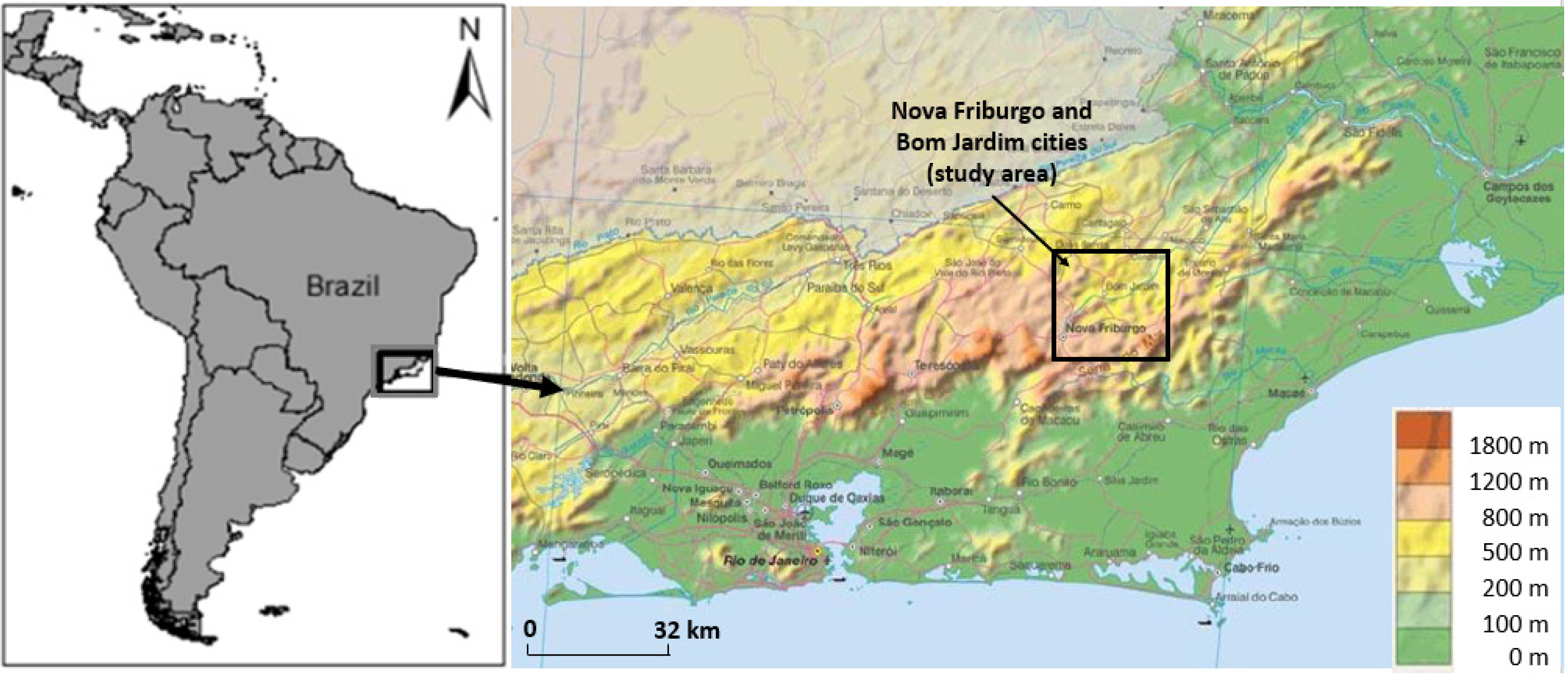
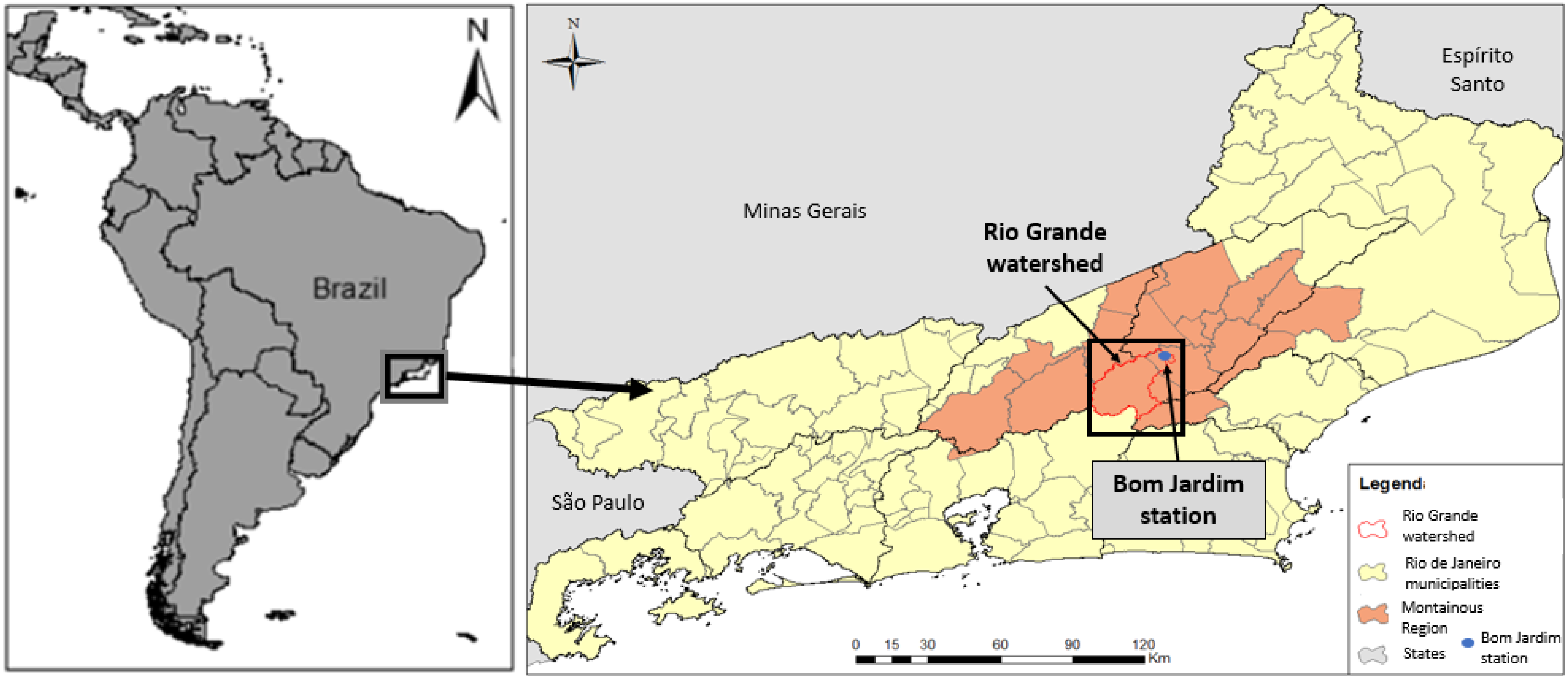
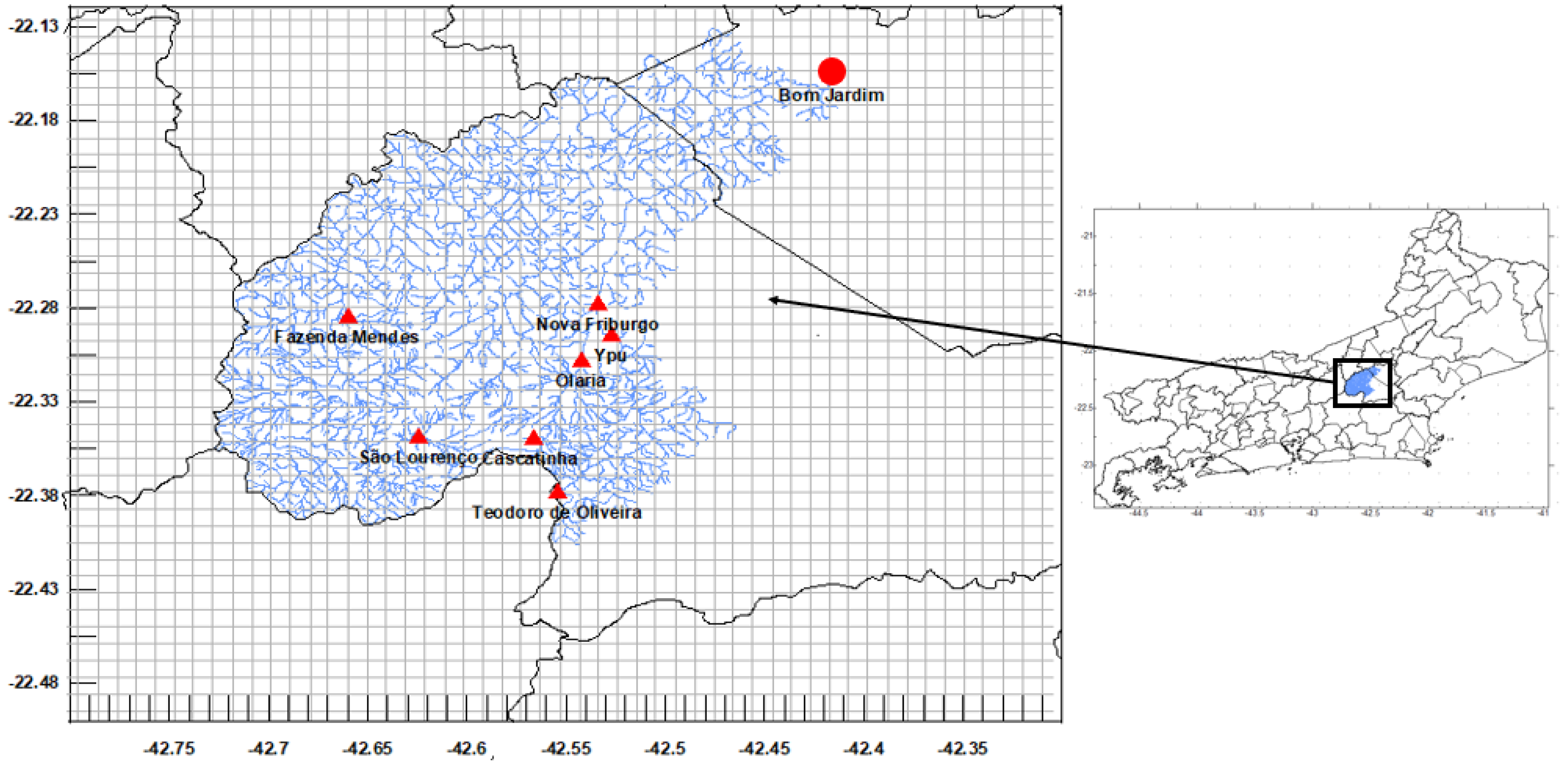
2.1. Study Area
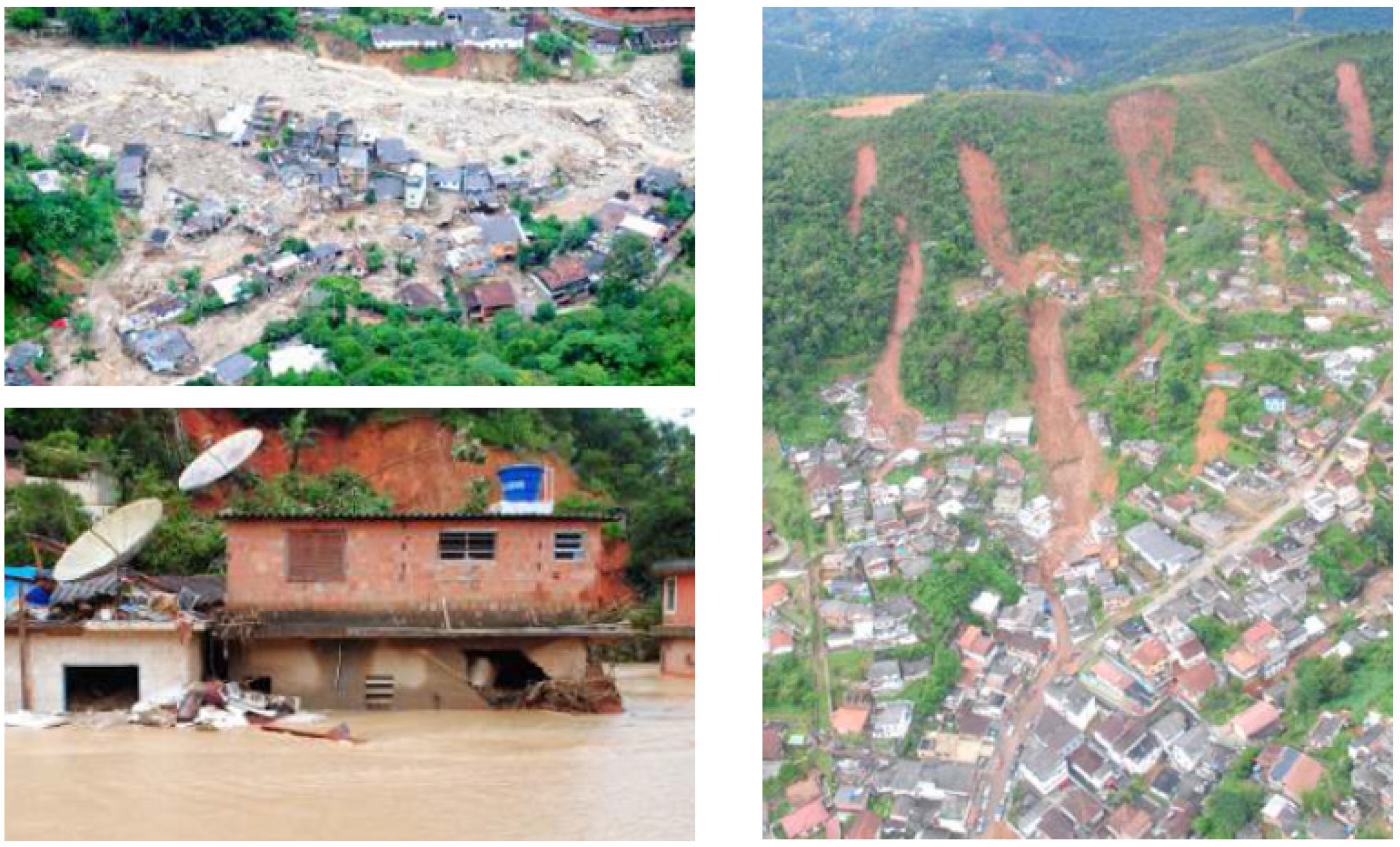
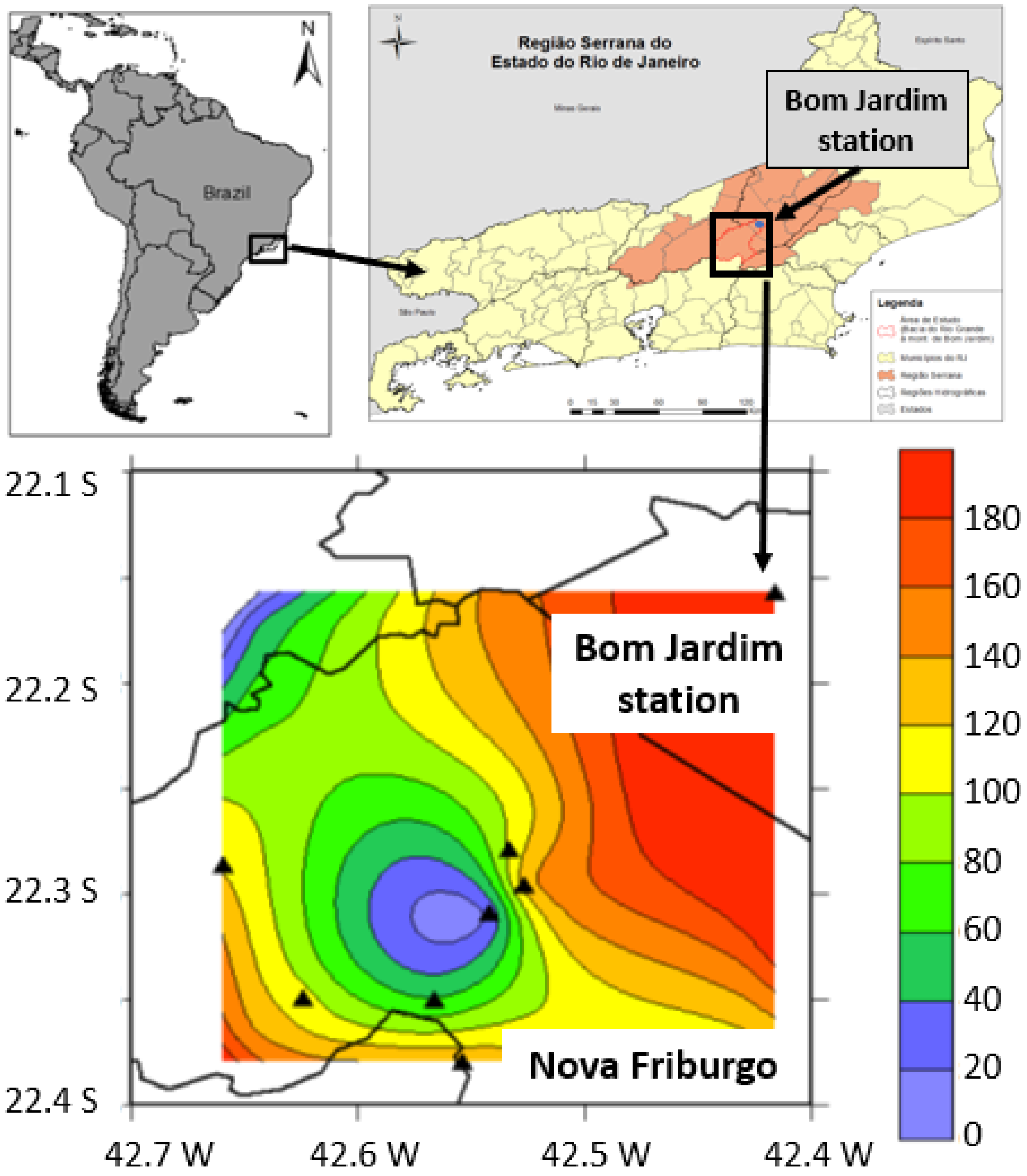
2.2. The Natural Hazard of 2011
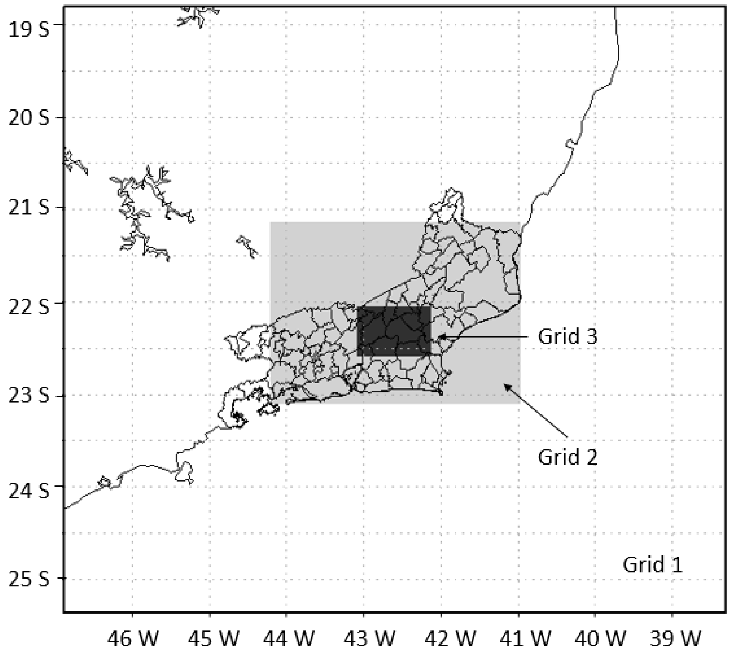
2.3. Precipitation: WRF Model
2.4. Floods: The SMAP Hydrological Model
3. Results
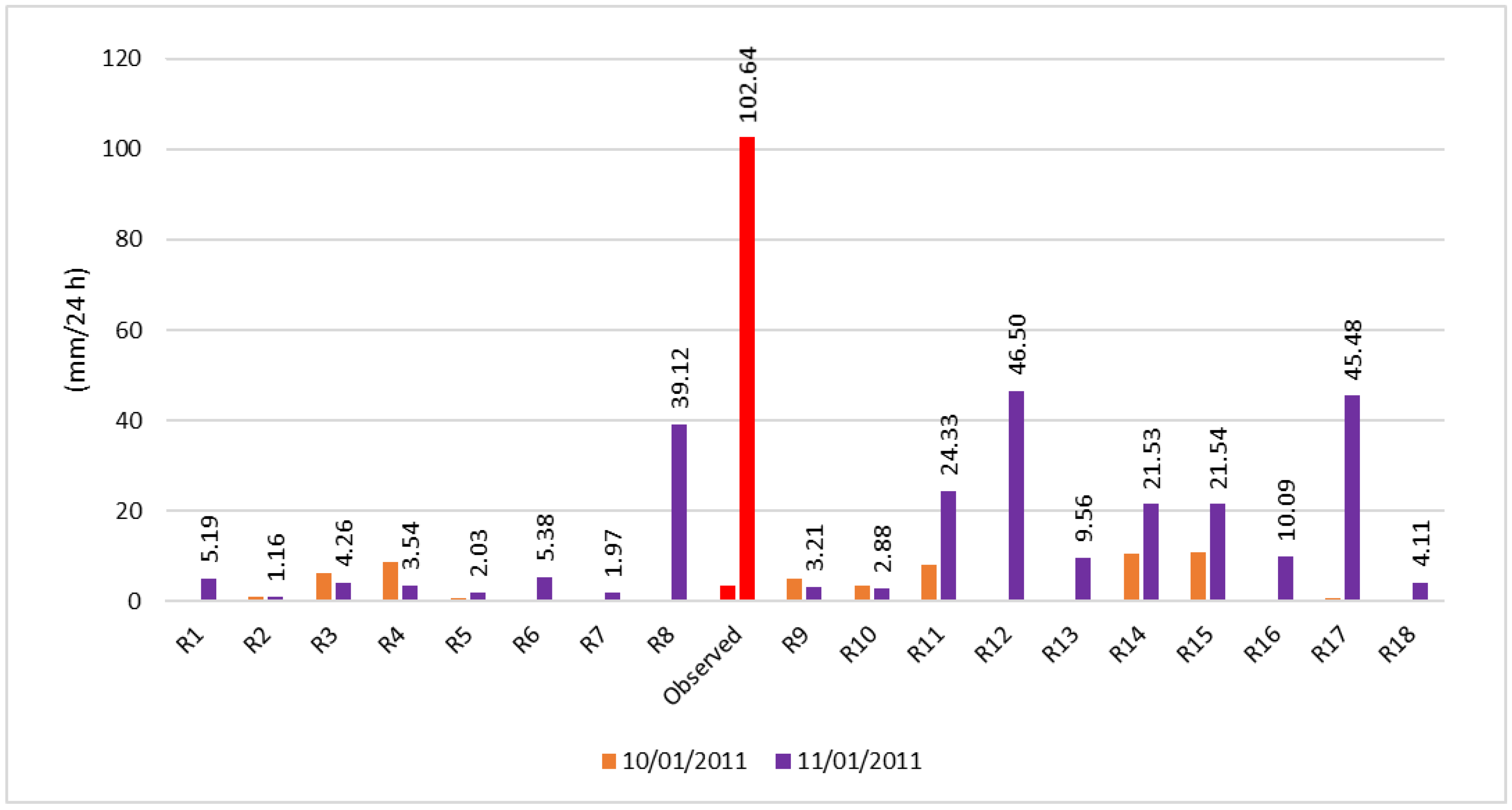
3.1. Meteorology
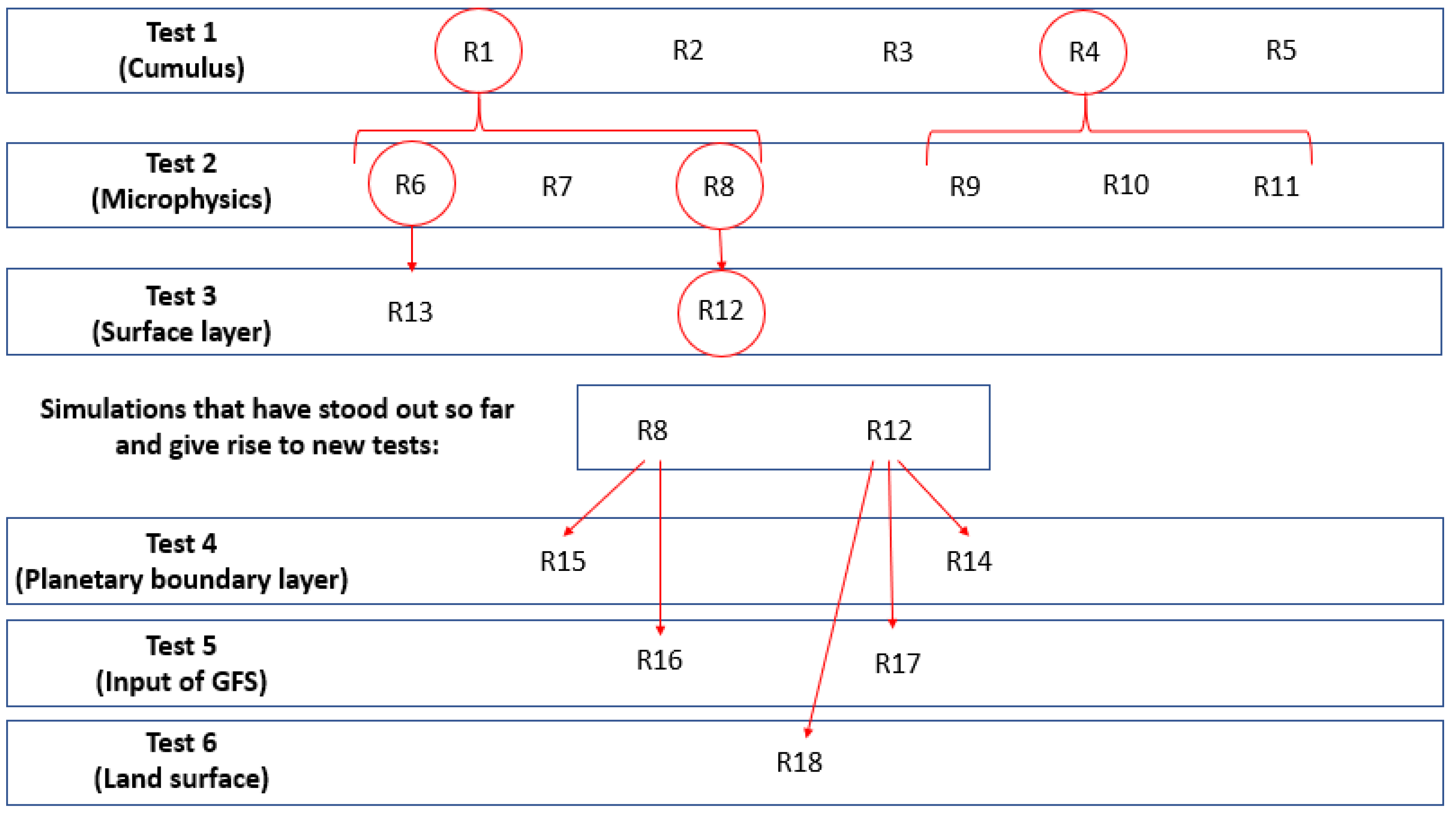
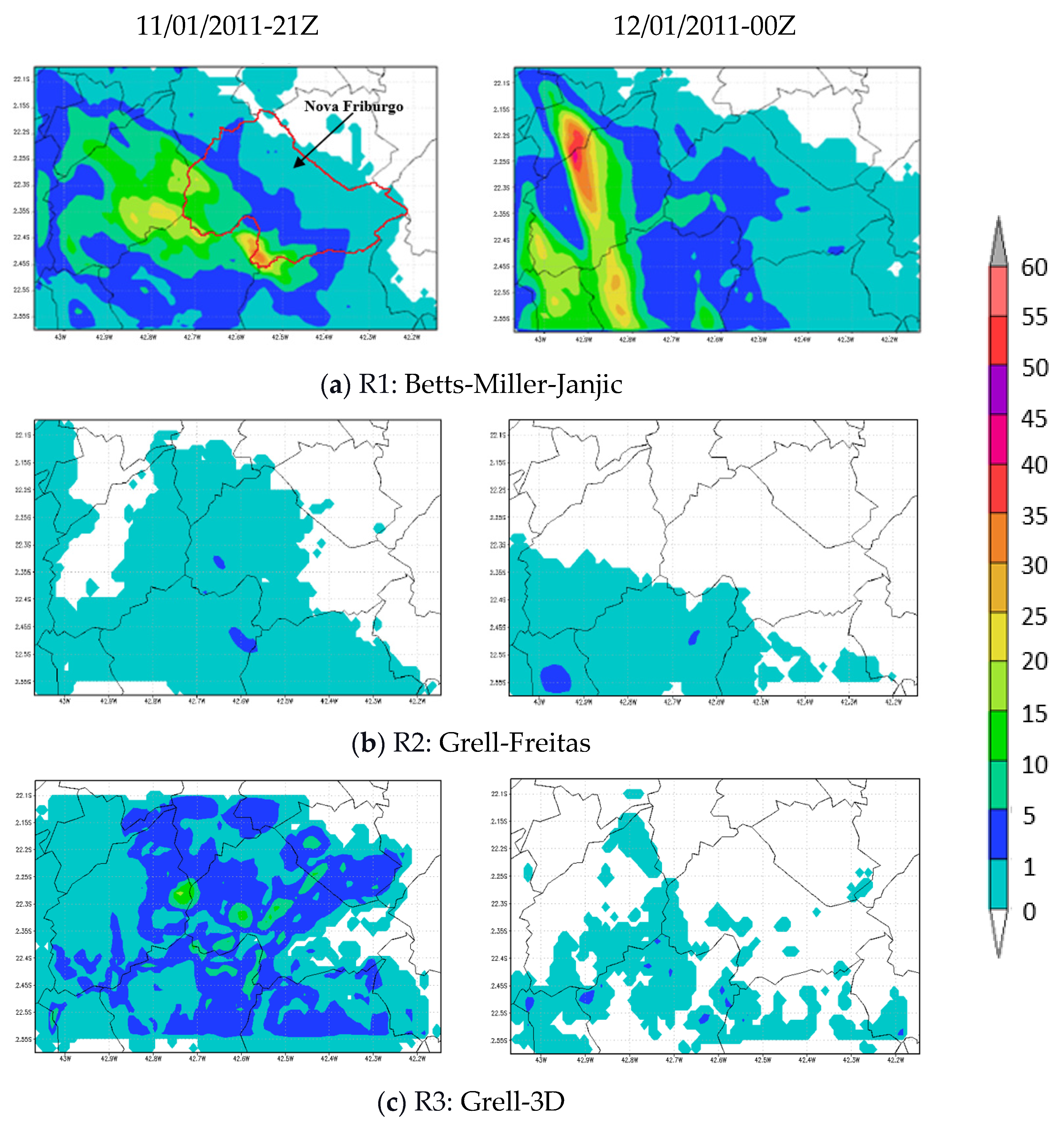
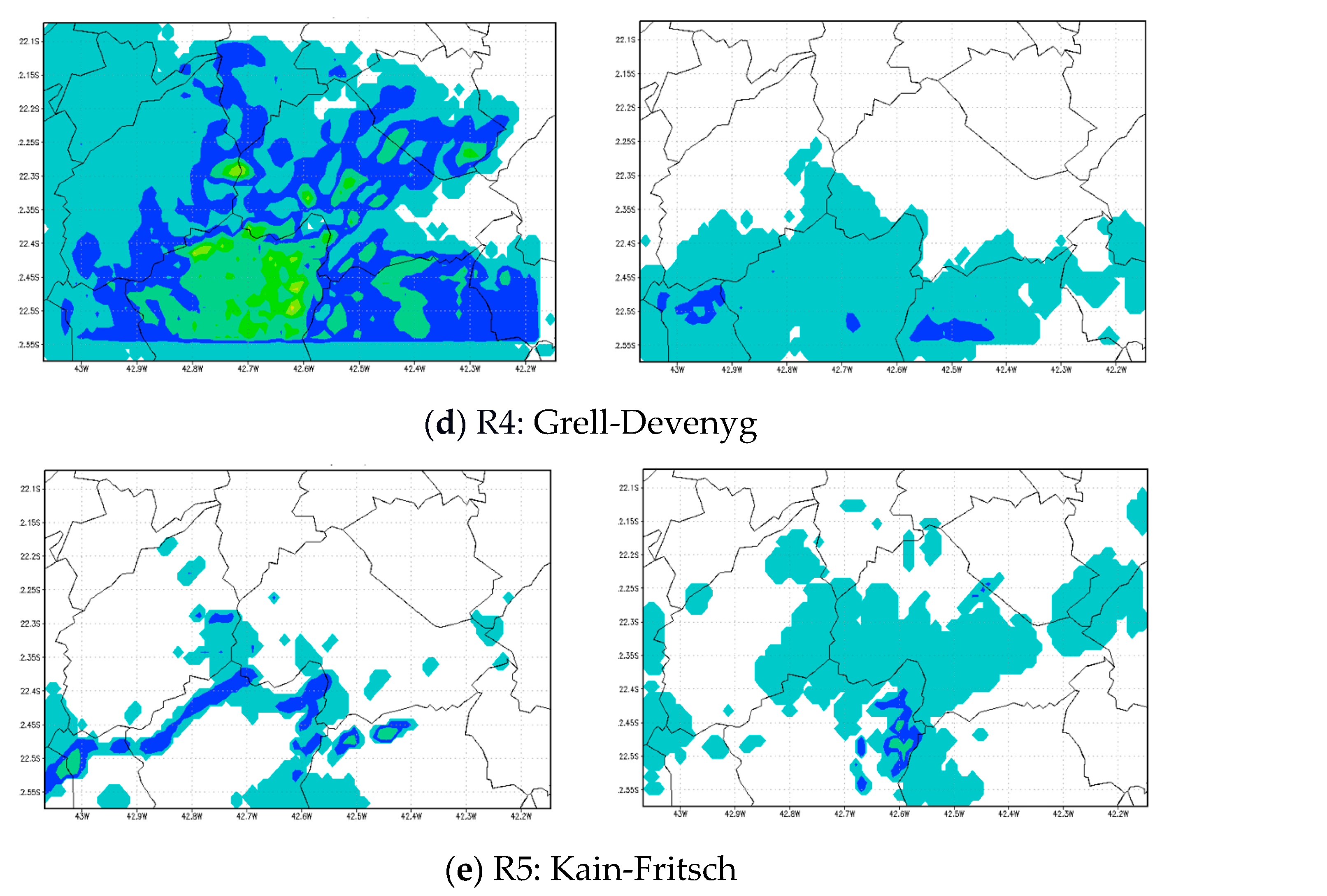
3.1.1. Test 1: Changing Cumulus Parametrization
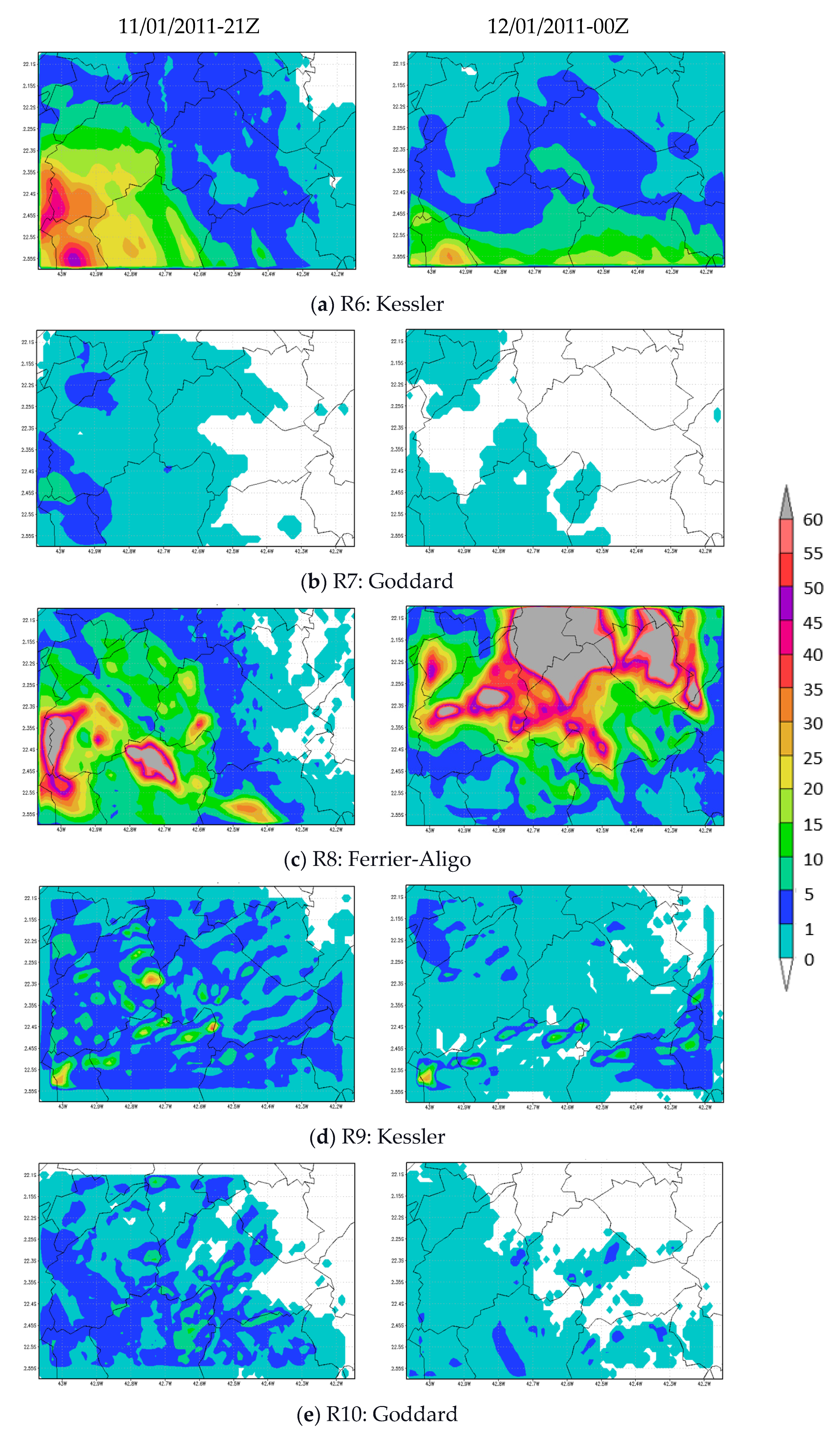
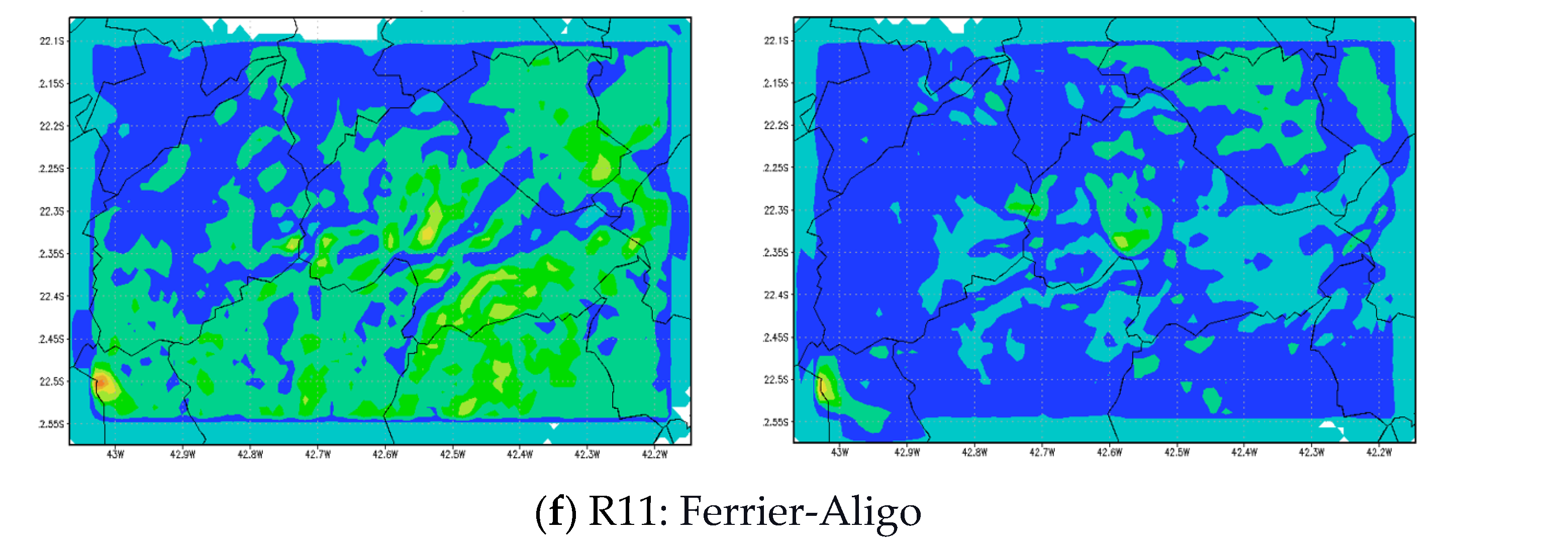
3.1.2. Test 2: Changing Microphysics Parametrization
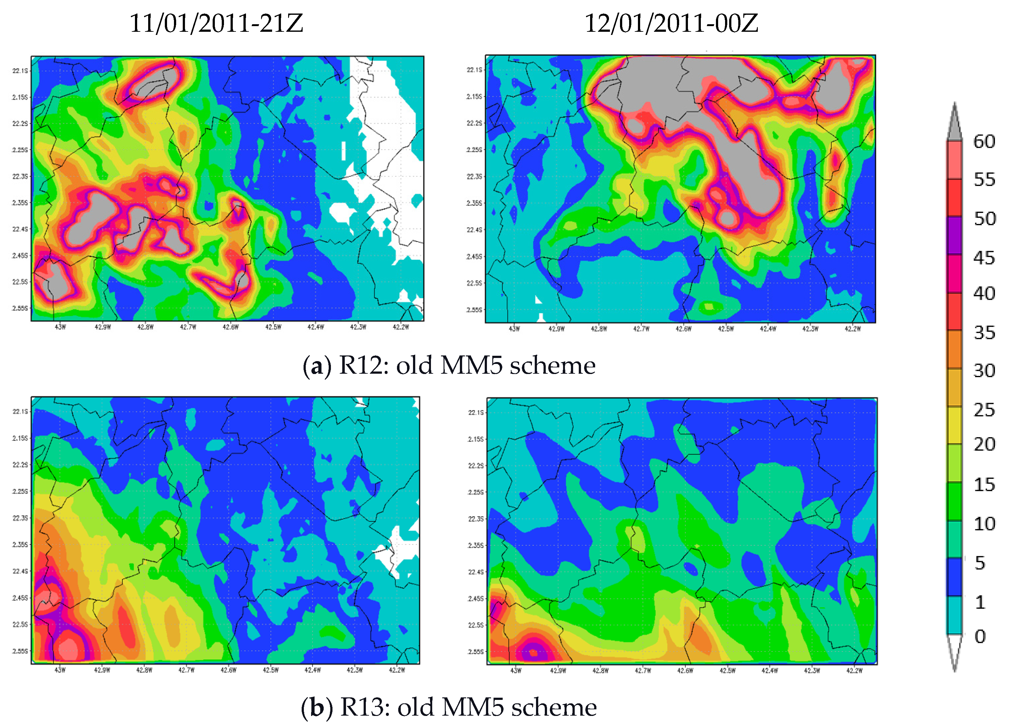
3.1.3. Test 3: Changing Surface Layer Parametrization
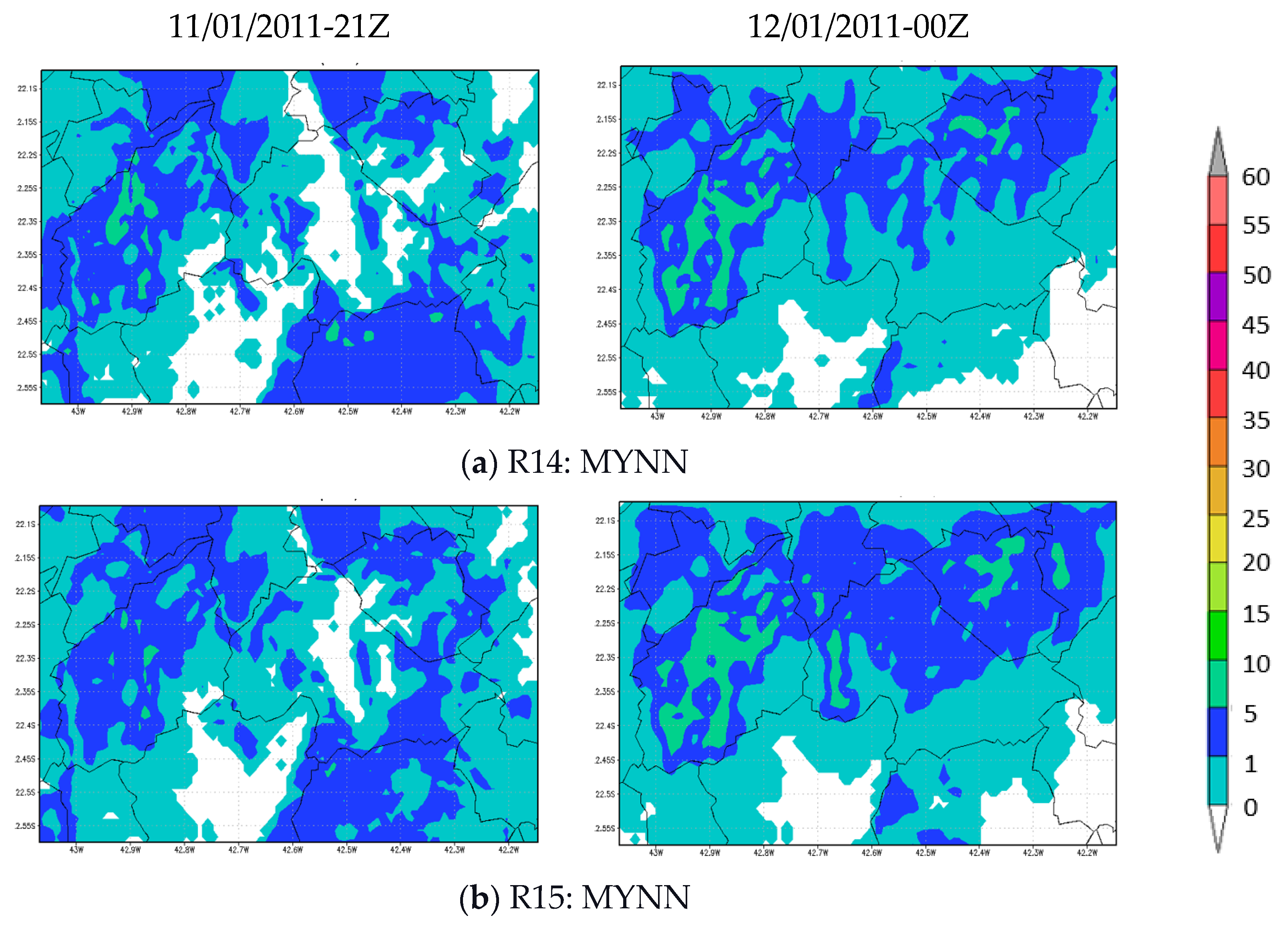
3.1.4. Test 4: Changing Planetary Boundary Layer Parametrization
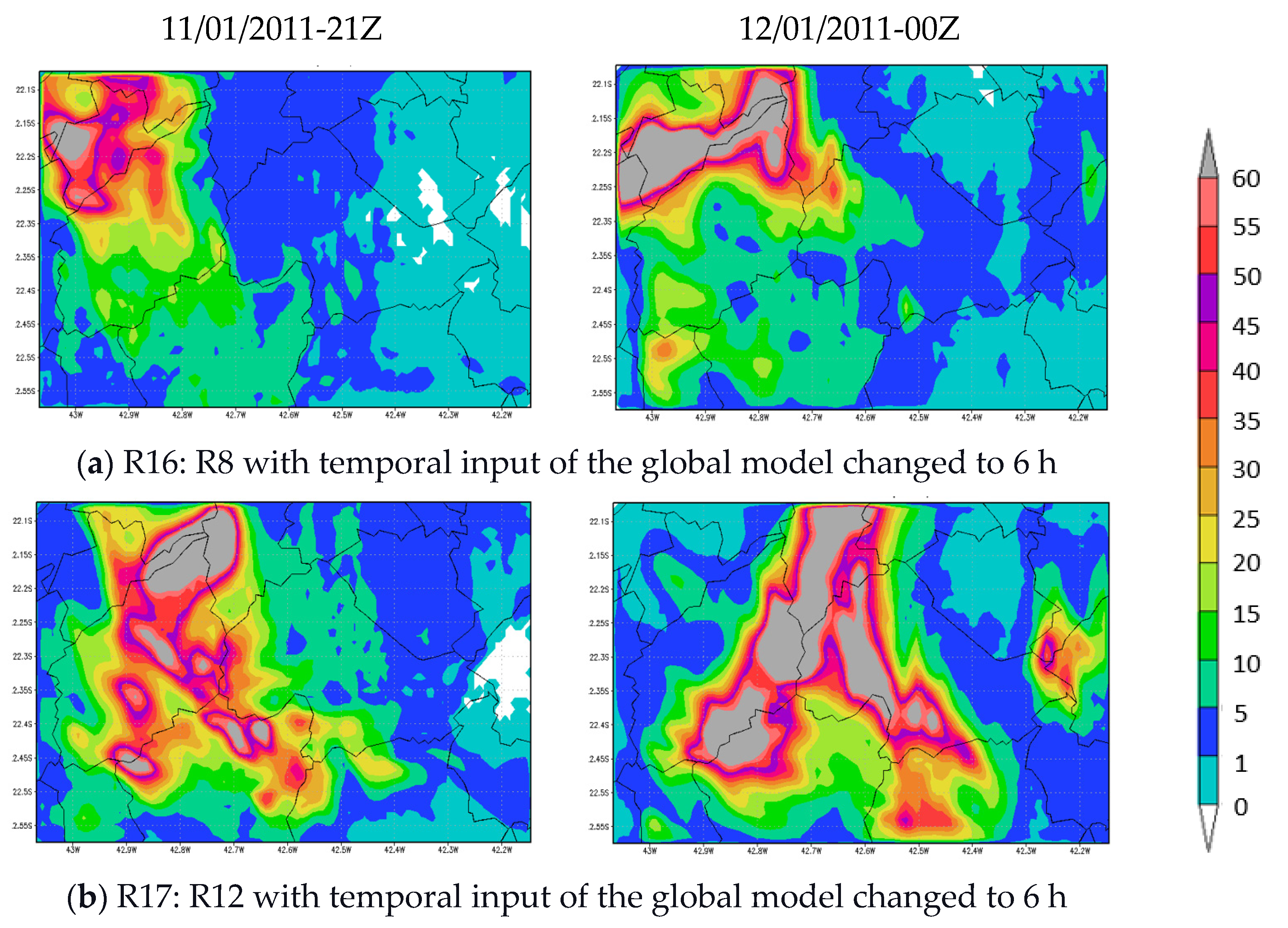
3.1.5. Test 5: Changing Input of GFS Model
3.1.6. Test 6: Changing Land Surface Parametrization
3.1.7. Changing Lead Time
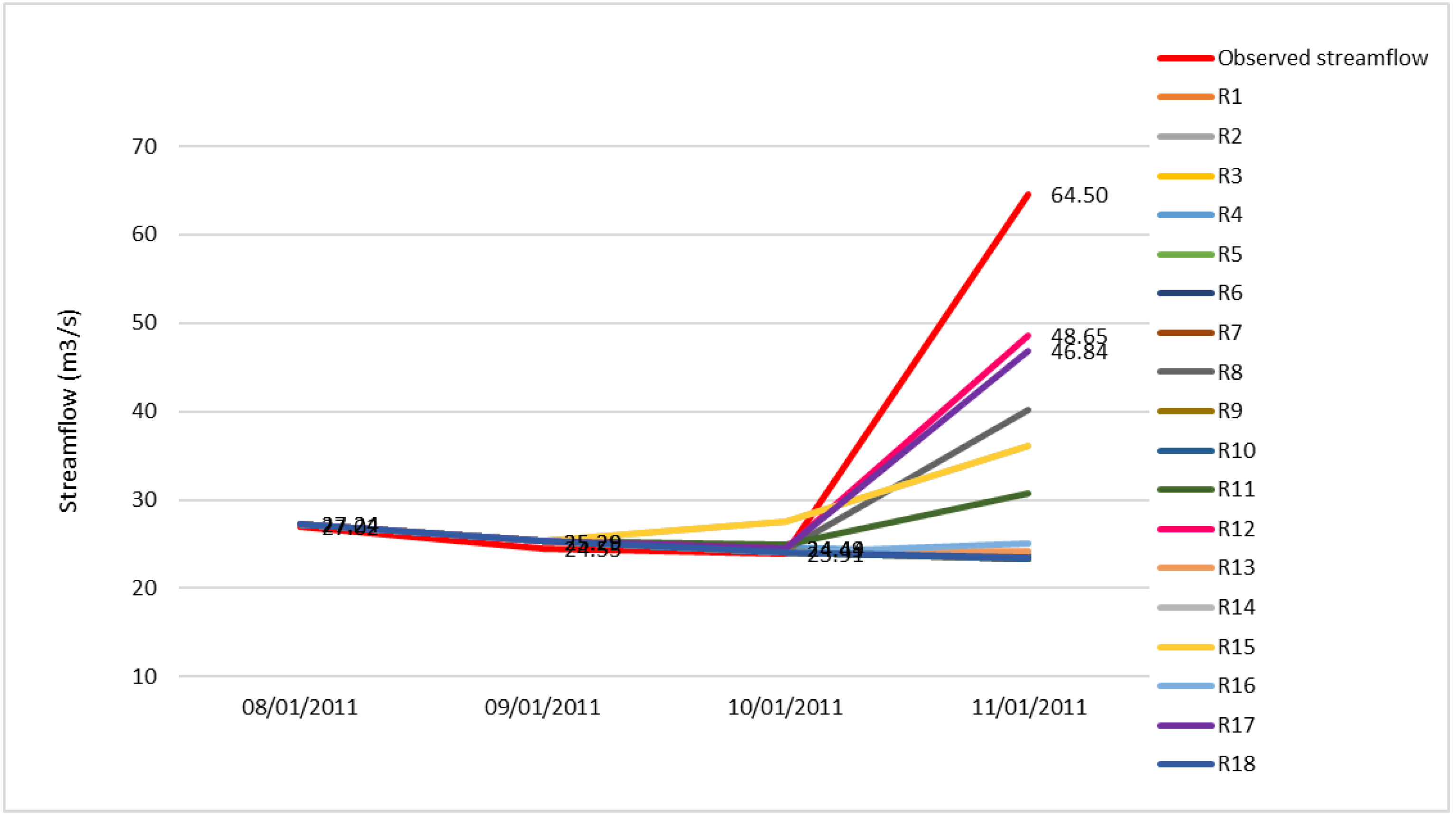
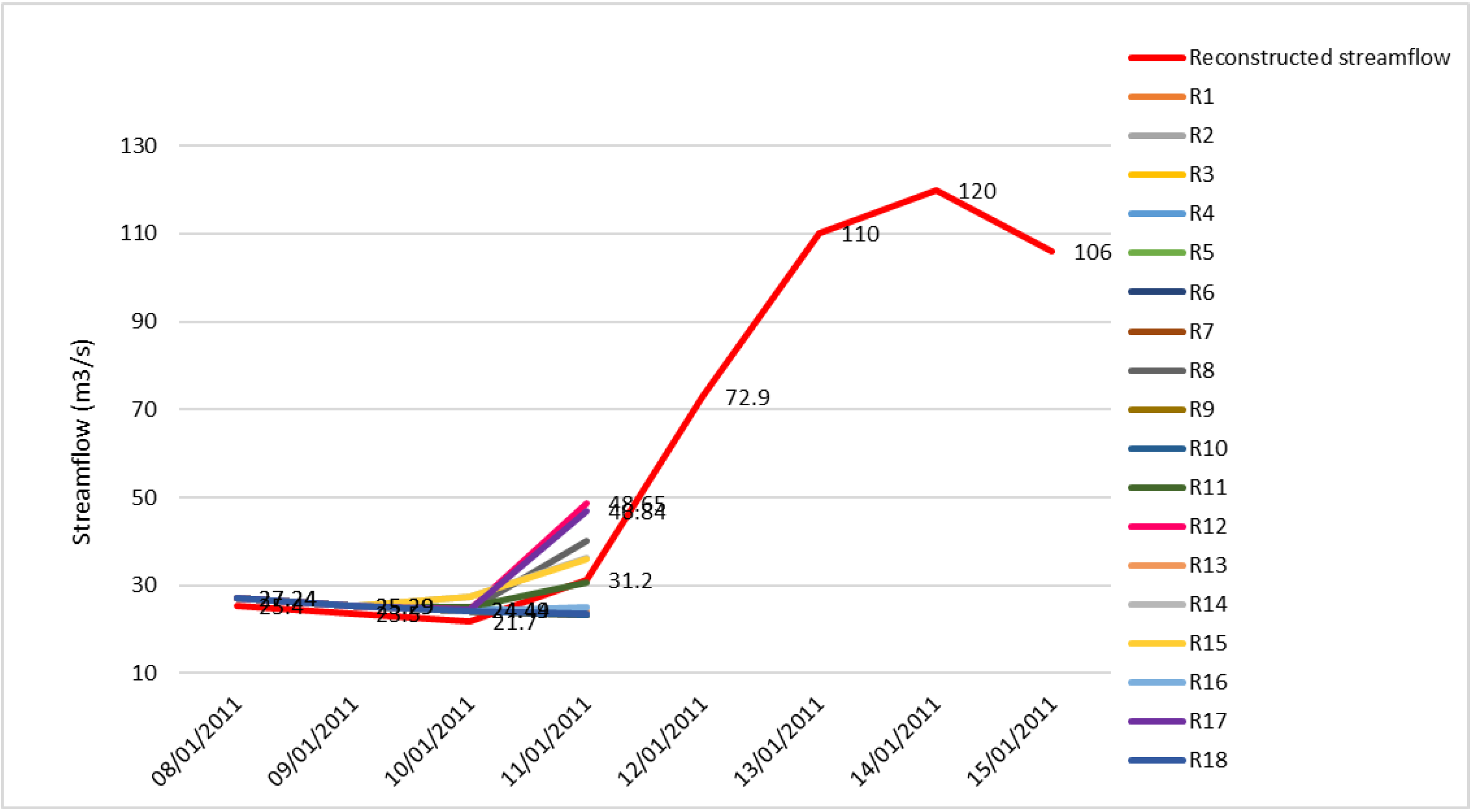
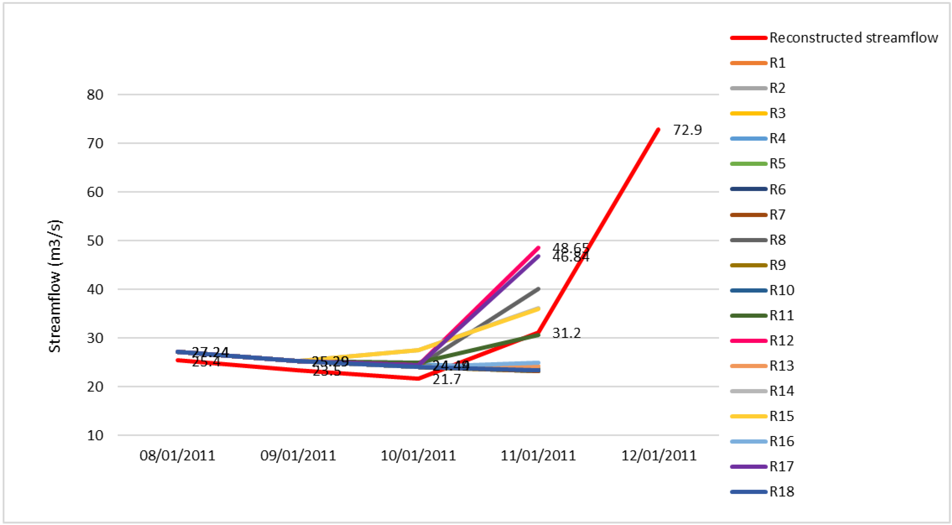
3.2. Hydrology
Forecasting Streamflow by the SMAP-WRF Ensemble
4. Discussion
5. Conclusions
Author Contributions
Funding
Conflicts of Interest
References
- World Bank, 2012: Loss and Damage Assessment: Floods and Landslides in the “Serrana” Region of Rio de Janeiro-January 2011. Available online: http://mi.gov.br/pt/c/document_library/get_file?uuid=74dde46c-544a-4bc4-a6e1-852d4c09be06&groupId=10157 (accessed on 14 March 2018).
- Moura, C.R.W.; Escobar, G.C.J.; Andrade, K.M. Padrões de circulação em superfície e altitude associados a eventos de chuva intensa na região metropolitana do Rio de Janeiro. Rev. Bras. Meteorol. 2013, 28, 267–280. [Google Scholar] [CrossRef]
- Viterbo, F.; Mahoney, K.; Read, L.; Salas, F.; Bates, B.; Elliott, J.; Cosgrove, B.; Dugger, A.; Gochis, D.; Cifelli, R. A Multiscale, Hydrometeorological Forecast Evaluation of National Water Model Forecasts of the May 2018 Ellicott City, Maryland, Flood. J. Hydrometeor. 2020, 21, 475–499. [Google Scholar] [CrossRef]
- NCAR, 2010: Flash Flood Early Warning System Reference Guide. Available online: https://www.meted.ucar.edu/communities/hazwarnsys/ffewsrg/FF_EWS.pdf (accessed on 3 November 2015).
- Sun, D.; Zhang, D.; Cheng, X. Framework of National Non-Structural Measures for Flash Flood Disaster Prevention in China. Water 2012, 4, 272–282. [Google Scholar] [CrossRef]
- Barcellos, P.C.L.; Da Costa, M.S.; Cataldi, M.; Soares, C.A.P. Management of non-structural measures in the prevention of flash floods: A case study in the city of Duque de Caxias, state of Rio de Janeiro, Brazil. Nat. Hazards 2017, 89, 313–330. [Google Scholar] [CrossRef]
- Faisal, I.M.; Kabir, M.R.; Nishat, A. Non-structural flood mitigation measures for Dhaka City. Urban Water 1999, 1, 145–153. [Google Scholar] [CrossRef]
- Calmant, S.; Lee, H.; Souza, A.E.; Shum, C.K.; Seyler, F.; Huang, Z.; Ries, J. JASON-2 IGDRs for Flood Alert in the Amazon Basin. In Proceedings of the Ocean Surface Topography Science Team Meeting, Seattle, WA, USA, 22–24 June 2009; Available online: http://depts.washington.edu/uwconf/ostst2009/OSTST_book_2009_Final.pdf (accessed on 2 April 2019).
- Ahnert, P. National Weather Service Flash Flood Warning Program. In Proceedings of the Internacional Workshop Early Warning for flash floods, Prague, Czech Republic, 2011; Available online: http://www.preventionweb.net/files/24455_ewflashfloods.pdf (accessed on 13 May 2019).
- Angerhofer, G. The Weather Warning System of German Weather Service Provider and Special Information for Disaster Control. In Proceedings of the Internacional Workshop Early Warning for flash floods, Prague, Czech Republic, 2011; Available online: http://www.preventionweb.net/files/24455_ewflashfloods.pdf (accessed on 13 May 2019).
- Danhelka, J. Hydrological Forecasting and Warning in Case of Flash Flood. In Proceedings of the Internacional Workshop Early Warning for flash floods, Prague, Czech Republic, 2011; Available online: http://www.preventionweb.net/files/24455_ewflashfloods.pdf (accessed on 13 May 2019).
- Gerard, F. State of Art with Flash Flood Early Warning and Management Capacities in France. In Proceedings of the Internacional Workshop Early Warning for flash floods, Prague, Czech Republic, 2011; Available online: http://www.preventionweb.net/files/24455_ewflashfloods.pdf (accessed on 13 May 2019).
- Adams, T.; Pagano, T. Flood Forecasting: A Global Perspective, 1st ed.; Academic Press: Cambridge, MA, USA, 2016; pp. 399–417. [Google Scholar]
- Looper, J.P.; Vieux, B.E. An assessment of distributed flash flood forecasting accuracy using radar and rain gauge input for a physics-based distributed hydrologic model. J. Hydrol. 2012, 412, 114–132. [Google Scholar] [CrossRef]
- Adams, T.E.; Dymond, R. The Effect of QPF on Real-Time Deterministic Hydrologic Forecast Uncertainty. J. Hydrometeor. 2019, 20, 1687–1705. [Google Scholar] [CrossRef]
- Tao, J.; Barros, A.P. Prospects for flash flood forecasting in mountainous regions – An investigation of Tropical Storm Fay in the Southern Appalachians. J. Hydrol. 2013, 506, 69–89. [Google Scholar] [CrossRef]
- Shamir, E.; Georgakakos, K.P.; Spencer, C.; Modrick, T.M.; Murphy, J.M.; Jubach, R. Evaluation of real-time flash flood forecasts for Haiti during the passage of Hurricane Tomas. Nat. Hazards 2013, 67, 459–482. [Google Scholar] [CrossRef]
- Senatore, A.; Mendicino, G. Fully coupled WRF-Hydro atmospheric-hydrological modeling in a Mediterranean catchment. In Proceedings of the 1st European fully coupled Atmospheric-hydrological modeling and WRF-HYDRO users Workshop, Cosenza, Itália, 2014; Available online: http://www.eco-hydrology.org/wrf-hydro2014/BookOfAbstracts.pdf (accessed on 10 June 2019).
- Shih, D.; Chen, C.; Yeh, G. Improving our understanding of flood forecasting using earlier hydro-meteorological intelligence. J. Hydrol. 2014, 512, 470–481. [Google Scholar] [CrossRef]
- Amengual, A.; Homar, V.; Jaume, O. Potential of a probabilistic hydrometeorological forecasting approach for the 28 September 2012 extreme flash flood in Murcia, Spain. Atmos. Res. 2015, 166, 10–23. [Google Scholar] [CrossRef]
- Fredj, E.; Givati, A. Application of a Coupled WRF-Hydro Model for Extreme Flood Events in the Mediterranean Basins. Geophys. Res. Abstr. 2015, 17, EGU2015-7121. [Google Scholar]
- Li, J.; Chen, Y.; Wang, H.; Qin, J.; Li, J.; Chiao, S. Extending flood forecasting lead time in a large watershed by coupling WRF QPF with a distributed hydrological model. Hydrol. Earth Syst. Sci. 2017, 21, 1279–1294. [Google Scholar] [CrossRef]
- Silva Dias, M.A.F. Sistemas de Mesoescala e Previsão de Tempo a Curto Prazo. Rev. Bras. Meteorol. 1987, 2, 133–150. [Google Scholar]
- Jankov, I.; Bao, J.; Neiman, P.J.; Schultz, P.J.; Yuan, H.; White, A.B. Evaluation and Comparison of Microphysical Algorithms in ARW-WRF Model Simulations of Atmospheric River Events Affecting the California Coast. J. Hydrometeor. 2009, 10, 847–870. [Google Scholar] [CrossRef]
- Yuan, X.; Liang, X.Z.; Wood, E. WRF ensemble downscaling seasonal forecasts of China winter precipitation during 1982−2008. Clim. Dyn. 2012, 39, 2014–2058. [Google Scholar] [CrossRef]
- Mooney, P.A.; Mulligan, F.J.; Fealy, R. Evaluation of the sensitivity of the weather research and forecasting model to parameterization schemes for regional climates of Europe over the period 1990–95. J. Clim. 2013, 26, 1002–1017. [Google Scholar] [CrossRef]
- Kala, J.; Andrys, J.; Lyons, T.J.; Foster, I.J.; Evans, B.J. Sensitivity of WRF to driving data and physics options on a seasonal time-scale for the southwest of Western Australia. Clim. Dyn. 2015, 44, 633–659. [Google Scholar] [CrossRef]
- Ratnam, J.V.; Behera, S.K.; Krishnan, R.; Doi, T.; Ratna, S.B. Sensitivity of Indian summer monsoon simulation to physical parameterization schemes in the WRF model. Clim. Res. 2017, 74, 43–66. [Google Scholar] [CrossRef]
- Attada, R.; Dasari, H.P.; Kunchala, R.K.; Langodan, S.; Niranjan Kumar, K.; Knio, O.; Hoteit, I. Evaluating Cumulus Parameterization Schemes for the Simulation of Arabian Peninsula Winter Rainfall. J. Hydrometeor. 2017, 21, 1089–1114. [Google Scholar] [CrossRef]
- Cavalcante, M.R.G.; Barcellos, P.L.; Cataldi, M. Flash flood in the mountainous region of Rio de Janeiro state (Brazil) in 2011: Part I—Calibration watershed through hydrological SMAP model. Nat. Hazards 2020, 102, 1117–1134. [Google Scholar] [CrossRef]
- Luz Barcellos, P.C. Desastres Naturais, Hidrometeorologia e Defesa Civil: A Sinergia entre a Ciência e a Operação para Salvar Vidas; Novas Edições Acadêmicas: Brazil, 2016. [Google Scholar]
- Altitude Rio de Janeiro Map. Available online: https://map-of-rio-de-janeiro.com/other-maps/altitude-rio-de-janeiro-map (accessed on 28 July 2020).
- Dourado, F.; Arraes, T.C.; Silva, M.F. The Mega hazard of the “Serrana” Region of Rio de Janeiro-the Causes of the Event, the Mechanisms of Mass Movements and the Spatial Distribution of Post-Disaster Reconstruction Investments. Yearbook Inst. Geosci. 2012, 35, 43–54. [Google Scholar] [CrossRef]
- Skamarock, W.C.; Klemp, J.B.; Dudhia, J.; Gill, D.O.; Barker, D.M.; Duda, M.G.; Huang, X.; Wang, W.; Powers, J.G. A description of the Advanced Research WRF version 3. NCAR Tech. Note NCAR/TN-475+STR 2008, 113. [Google Scholar] [CrossRef]
- Global Forecast System (GFS). Available online: https://www.ncdc.noaa.gov/data-access/model-data/model-datasets/global-forcast-system-gfs (accessed on 29 July 2020).
- Janjić, Z.I. The Step-Mountain Eta Coordinate Model: Further Developments of the Convection, Viscous Sublayer, and Turbulence Closure Schemes. Mon. Weather Rev. 1994, 122, 927–945. [Google Scholar] [CrossRef]
- Grell, G.A.; Freitas, S.R. A scale and aerosol aware stochastic convective parameterization for weather and air quality modeling. Atmos. Chem. Phys. 2014, 14, 5233–5250. [Google Scholar] [CrossRef]
- Grell, G.A. Prognostic Evaluation of Assumptions Used by Cumulus Parameterizations. Mon. Weather Rev. 1993, 121, 764–787. [Google Scholar] [CrossRef]
- Grell, G.A.; Devenyi, D. A generalized approach to parameterizing convection combining ensemble and data assimilation techniques. Geophys. Res. Lett. 2002, 29, 38-1–38-4. [Google Scholar] [CrossRef]
- Kain, J.S. The Kain-Fritsch Convective Parameterization: An Update. J. Appl. Meteorol. 2004, 43, 170–181. [Google Scholar] [CrossRef]
- Hong, S.Y.; Lim, J.O.J. The WRF single-moment 6-class microphysics scheme (WSM6). Asia Pac. J. Atmos. Sci. 2006, 42, 129–151. [Google Scholar]
- Kessler, E. On the Distribution and Continuity of Water Substance in Atmospheric Circulations. Am. Meteorol. Soc. 1969, 10, 1–84. [Google Scholar]
- Tao, W.K.; Simpson, J.; McCumber, M. An Ice-Water Saturation Adjustment. Mon. Weather Rev. 1989, 117, 231–235. [Google Scholar] [CrossRef]
- Aligo, E.A.; Ferrier, B.; Carley, J.R. Modified NAM Microphysics for Forecasts of Deep Convective Storms. Mon. Weather Rev. 2018, 146, 4115–4153. [Google Scholar] [CrossRef]
- Jiménez, P.A.; Dudhia, J.; González-Rouco, J.F.; Navarro, J.; Montávez, J.P.; García-Bustamante, E. A Revised Scheme for the WRF Surface Layer Formulation. Mon. Weather Rev. 2012, 140, 898–918. [Google Scholar] [CrossRef]
- Paulson, C.A. The mathematical representation of wind speed and temperature profiles in the unstable atmospheric surface layer. J. Appl. Meteorol. 1970, 9, 857–861. [Google Scholar] [CrossRef]
- Hong, S.Y.; Pan, H.L. Nonlocal boundary layer vertical diffusion in a medium–range forecast model. Mon. Weather Rev. 1996, 124, 2322–2339. [Google Scholar] [CrossRef]
- Nakanishi, M.; Niino, H. An Improved Mellor–Yamada Level-3 Model: Its Numerical Stability and Application to a Regional Prediction of Advection Fog. Bound. Layer Meteorol. 2006, 119, 397–407. [Google Scholar] [CrossRef]
- Nakanishi, M.; Niino, H. Development of an improved turbulence closure model for the atmospheric boundary layer. J. Meteor. Soc. Jpn. 2009, 87, 895–912. [Google Scholar] [CrossRef]
- Dudhia, J. A multi-layer soil temperature model for MM5. In Proceedings of the sixth PSU/NCAR Mesoscale Model Users Worshop, Boulder, CO, USA, 22–24 July 1996. [Google Scholar]
- Lopes, J.E.G.; Braga, B.P.F.; Conejo, J.G.L. SMAP-a simplifed hydrological model. In Applied Modelling in Catchment Hydrology; Singh, V.P., Ed.; Water Resources Publications: Lone Tree, CO, USA, 1982; pp. 167–176. [Google Scholar]
- Janjić, Z.I. Comments on “Development and evaluation of a convection scheme for use in climate models”. J. Atmos. Sci. 2000, 57, 3686. [Google Scholar] [CrossRef]
- Padilha, S.F. Simulações de Eventos de Chuvas Intensas no Estado do Rio de Janeiro Usando o Modelo WRF. Master’s Thesis, Universidade Federal do Rio de Janeiro, Rio de Janeiro, Brazil, 2011. [Google Scholar]
- Ryan, B.F. On the global variation of precipitating layer clouds. Bull. Am. Meteorol. Soc. 1996, 77, 53–70. [Google Scholar] [CrossRef][Green Version]
- GATE Reports. Bull. Am. Meteorol. Soc. 1974, 55, 711–744. Available online: https://www.jstor.org/stable/i26253638 (accessed on 6 August 2020). [CrossRef]
- Dye, J.E.; Jones, J.J.; Winn, W.P.; Cerni, T.A.; Gardiner, B.; Lamb, D.; Pitter, R.L.; Hallett, J.; Saunders, C.P.R. Early electrification and precipitation development in a small, isolated Montana cumulonimbus. J. Geophys. Res. Atmos. 1986, 91, 1231–1247. [Google Scholar] [CrossRef]
- Costa, A.A.; De Oliveira, J.C.; De Oliveira, J.C.P.; Sampaio, A.J.C. Microphysical Observations of Warm Cumulus Clouds in Ceará, Brazil. Atmos. Res. 2000, 54, 167–199. [Google Scholar] [CrossRef]


| Simulations | Cumulus Parameterization | Microphysics Parameterization | Surface Layer Parameterization | PBL Parameterization | Land Surface Parameterization |
|---|---|---|---|---|---|
| Test 1: Changing in cumulus parametrization (cu_physics) | |||||
| R1 | 2 (Betts-Miller-Janjic) | 6 (wsm6) | 1 (MM5) | 99 (MRF) | 4 (Noah MP) |
| R2 | 3 (Grell-Freitas) | 6 (wsm6) | 1 (MM5) | 99 (MRF) | 4 (Noah MP) |
| R3 | 5 (Grell-3D) | 6 (wsm6) | 1 (MM5) | 99 (MRF) | 4 (Noah MP) |
| R4 | 93 (Grell-Devenyg) | 6 (wsm6) | 1 (MM5) | 99 (MRF) | 4 (Noah MP) |
| R5 | 1 (Kain-Fritsch) | 6 (wsm6) | 1 (MM5) | 99 (MRF) | 4 (Noah MP) |
| Test 2: Changing in microphysics parameterization (mp_physics) | |||||
| R6 | 2 (Betts-Miller-Janjic) | 1 (Kessler) | 1 (MM5) | 99 (MRF) | 4 (Noah MP) |
| R7 | 2 (Betts-Miller-Janjic) | 7 (Goddard) | 1 (MM5) | 99 (MRF) | 4 (Noah MP) |
| R8 | 2 (Betts-Miller-Janjic) | 5 (Ferrier-Aligo) | 1 (MM5) | 99 (MRF) | 4 (Noah MP) |
| R9 | 93 (Grell-Devenyg) | 1 (Kessler) | 1 (MM5) | 99 (MRF) | 4 (Noah MP) |
| R10 | 93 (Grell-Devenyg) | 7 (Goddard) | 1 (MM5) | 99 (MRF) | 4 (Noah MP) |
| R11 | 93 (Grell-Devenyg) | 5 (Ferrier-Aligo) | 1 (MM5) | 99 (MRF) | 4 (Noah MP) |
| Test 3: Changing in surface layer parameterization (sf_sfclay_physics) | |||||
| R12 | 2 (Betts-Miller-Janjic) | 5 (Ferrier-Aligo) | 91 (MM5 old) | 99 (MRF) | 4 (Noah MP) |
| R13 | 2 (Betts-Miller-Janjic) | 1 (Kessler) | 91 (MM5 old) | 99 (MRF) | 4 (Noah MP) |
| Test 4: Changing in the PBL parameterization (bl_pbl_physics) | |||||
| R14 | 2 (Betts-Miller-Janjic) | 5 (Ferrier-Aligo) | 91 (MM5 old) | 6 (MYJ) | 4 (Noah MP) |
| R15 | 2 (Betts-Miller-Janjic) | 5 (Ferrier-Aligo) | 1 (MM5) | 6 (MYJ) | 4 (Noah MP) |
| Test 5: Changing the input of GFS model to 6 h | |||||
| R16 | 2 (Betts-Miller-Janjic) | 5 (Ferrier-Aligo) | 1 (MM5) | 99 (MRF) | 4 (Noah MP) |
| R17 | 2 (Betts-Miller-Janjic) | 5 (Ferrier-Aligo) | 91 (MM5 old) | 99 (MRF) | 4 (Noah MP) |
| Test 6: Changing the land surface parameterization (sf_surface_physics) | |||||
| R18 | 2 (Betts-Miller-Janjic) | 5 (Ferrier-Aligo) | 91 (MM5 old) | 99 (MRF) | 1 (Dudhia, 1996) |
© 2020 by the authors. Licensee MDPI, Basel, Switzerland. This article is an open access article distributed under the terms and conditions of the Creative Commons Attribution (CC BY) license (http://creativecommons.org/licenses/by/4.0/).
Share and Cite
da Cunha Luz Barcellos, P.; Cataldi, M. Flash Flood and Extreme Rainfall Forecast through One-Way Coupling of WRF-SMAP Models: Natural Hazards in Rio de Janeiro State. Atmosphere 2020, 11, 834. https://doi.org/10.3390/atmos11080834
da Cunha Luz Barcellos P, Cataldi M. Flash Flood and Extreme Rainfall Forecast through One-Way Coupling of WRF-SMAP Models: Natural Hazards in Rio de Janeiro State. Atmosphere. 2020; 11(8):834. https://doi.org/10.3390/atmos11080834
Chicago/Turabian Styleda Cunha Luz Barcellos, Priscila, and Marcio Cataldi. 2020. "Flash Flood and Extreme Rainfall Forecast through One-Way Coupling of WRF-SMAP Models: Natural Hazards in Rio de Janeiro State" Atmosphere 11, no. 8: 834. https://doi.org/10.3390/atmos11080834
APA Styleda Cunha Luz Barcellos, P., & Cataldi, M. (2020). Flash Flood and Extreme Rainfall Forecast through One-Way Coupling of WRF-SMAP Models: Natural Hazards in Rio de Janeiro State. Atmosphere, 11(8), 834. https://doi.org/10.3390/atmos11080834