Role of Horizontal Eddy Diffusivity within the Canopy on Fire Spread

 ,
,  , and
, and
Abstract
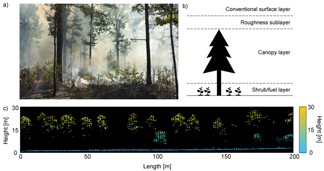
1. Introduction
2. Materials and Methods
2.1. Data
2.2. Theoretical Formulation
2.2.1. Horizontal Wind
2.2.2. Horizontal Diffusivity
3. Results
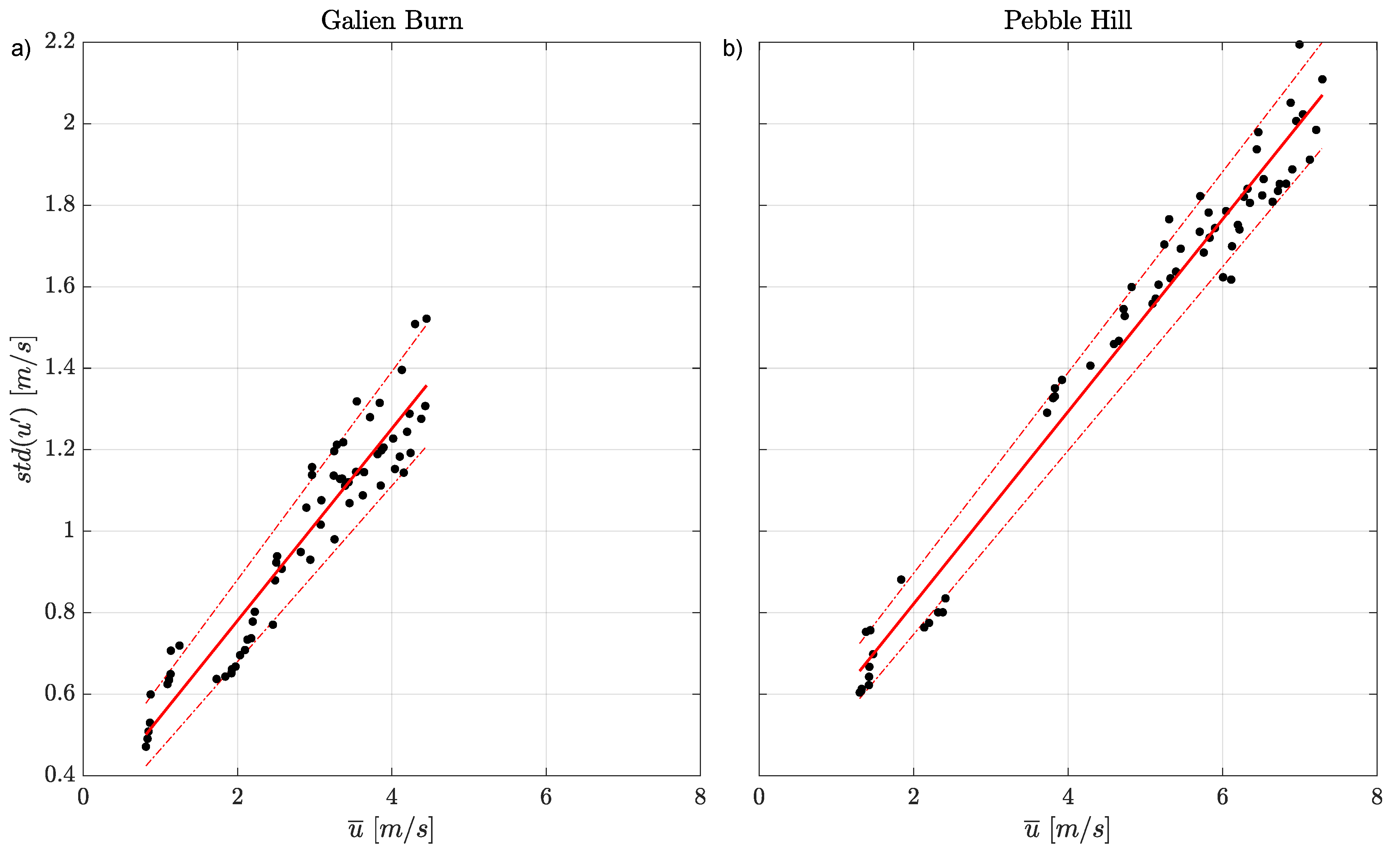
3.1. Vertical Profile of Horizontal Wind
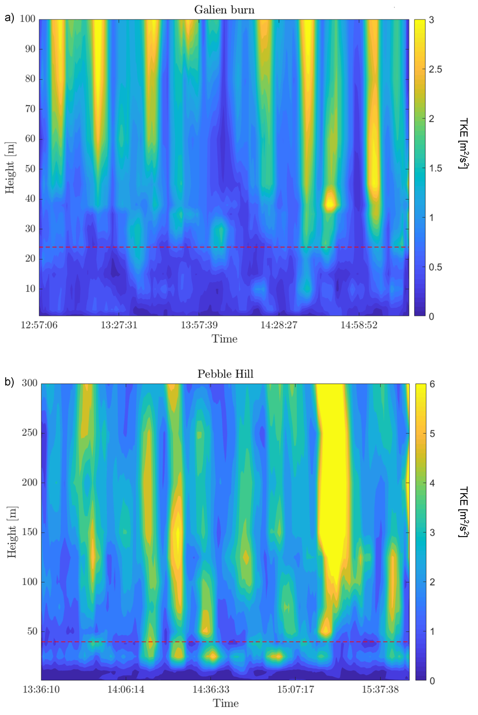
3.2. Vertical Structure of Turbulent Kinetic Energy
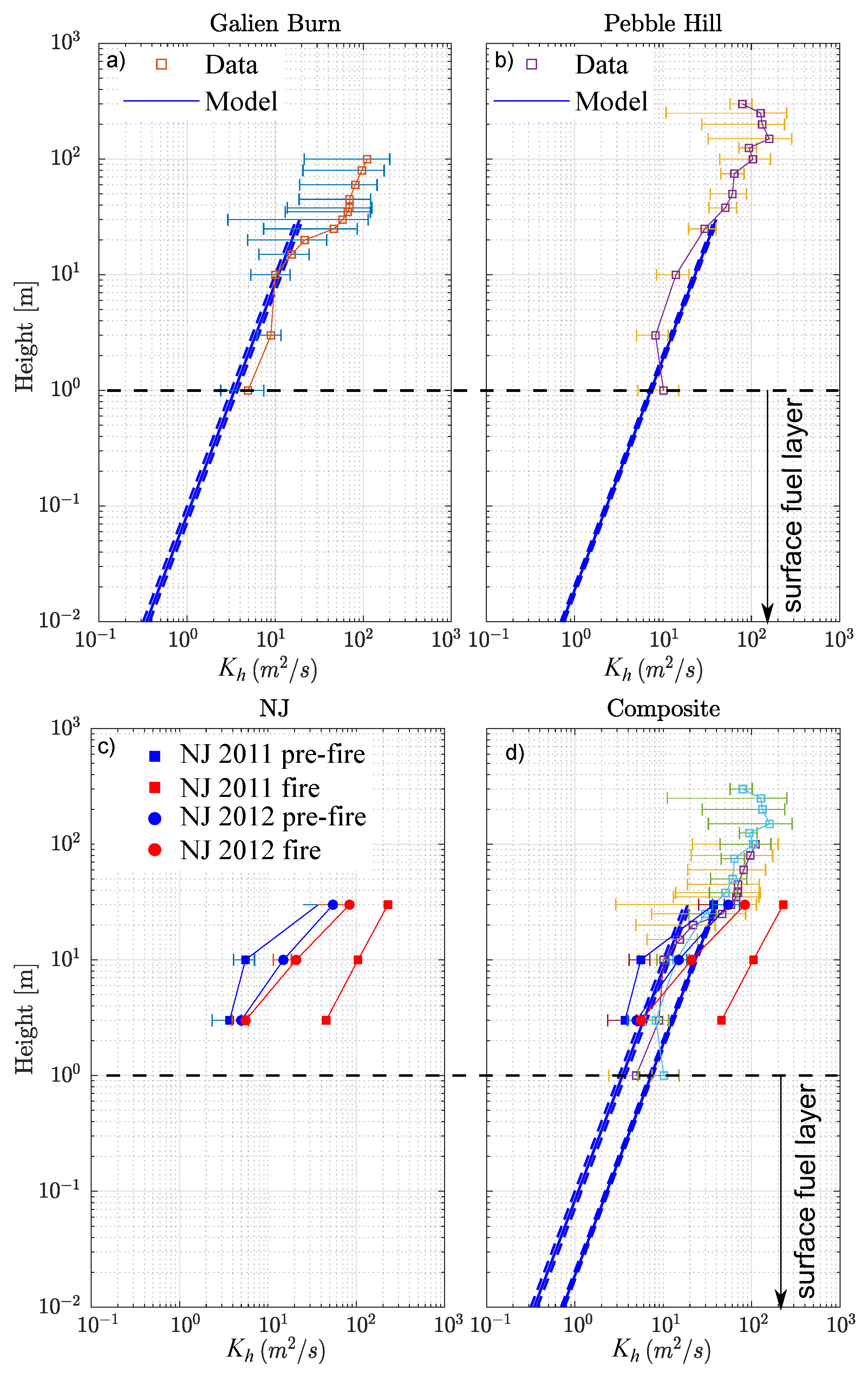
3.3. Horizontal Diffusivity
4. Advection-Diffusion-Reaction Model
4.1. Model Setup
4.2. Model Solution
5. Discussion
6. Conclusions
Author Contributions
Funding
Acknowledgments
Conflicts of Interest
References
- Lee, X. Turbulence spectra and eddy diffusivity over forests. J. Appl. Meteorol. 1996, 35, 1307–1318. [Google Scholar] [CrossRef]
- Clements, C.B.; Zhong, S.; Bian, X.; Heilman, W.E.; Byun, D.W. First observations of turbulence generated by grass fires. J. Geophys. Res. Atmos. 2008, 113. [Google Scholar] [CrossRef]
- Raupach, M.; Thom, A.S. Turbulence in and above plant canopies. Annu. Rev. Fluid Mech. 1981, 13, 97–129. [Google Scholar] [CrossRef]
- Harman, I.N.; Finnigan, J.J. A simple unified theory for flow in the canopy and roughness sublayer. Bound.-Layer Meteorol. 2007, 123, 339–363. [Google Scholar] [CrossRef]
- Raupach, M.; Finnigan, J.; Brunet, Y. Coherent eddies and turbulence in vegetation canopies: The mixing-layer analogy. In Boundary-Layer Meteorology 25th Anniversary Volume, 1970–1995; Springer: Berlin/Heidelberg, Germany, 1996; pp. 351–382. [Google Scholar]
- Finnigan, J. Turbulence in plant canopies. Annu. Rev. Fluid Mech. 2000, 32, 519–571. [Google Scholar] [CrossRef]
- Bai, K.; Katz, J.; Meneveau, C. Turbulent flow structure inside a canopy with complex multi-scale elements. Bound.-Layer Meteorol. 2015, 155, 435–457. [Google Scholar] [CrossRef]
- Moon, K.; Duff, T.; Tolhurst, K. Sub-canopy forest winds: Understanding wind profiles for fire behaviour simulation. Fire Saf. J. 2019, 105, 320–329. [Google Scholar] [CrossRef]
- Heilman, W.E.; Zhong, S.; Hom, J.L.; Charney, J.J.; Kiefer, M.T.; Clark, K.L.; Skowronski, N.; Bohrer, G.; Lu, W.; Liu, Y.; et al. Development of Modeling Tools for Predicting Smoke Dispersion from Low-Intensity Fires; Final Report, U.S. Joint Fire Science Program, Project 09–1-04-1; U.S. Joint Fire Science Program: Boise, ID, USA, 2013.
- Heilman, W.E.; Clements, C.B.; Seto, D.; Bian, X.; Clark, K.L.; Skowronski, N.S.; Hom, J.L. Observations of fire-induced turbulence regimes during low-intensity wildland fires in forested environments: Implications for smoke dispersion. Atmos. Sci. Lett. 2015, 16, 453–460. [Google Scholar] [CrossRef]
- LeMone, M.A.; Angevine, W.M.; Bretherton, C.S.; Chen, F.; Dudhia, J.; Fedorovich, E.; Katsaros, K.B.; Lenschow, D.H.; Mahrt, L.; Patton, E.G.; et al. 100 Years of Progress in Boundary Layer Meteorology. Meteorol. Monogr. 2019, 59, 9.1–9.85. [Google Scholar] [CrossRef]
- Lee, X. Fundamentals of Boundary-Layer Meteorology; Springer: Berlin/Heidelberg, Germany, 2018. [Google Scholar]
- Arya, P.S. Introduction to Micrometeorology; Elsevier: Amsterdam, The Netherlands, 2001; Volume 79. [Google Scholar]
- Draper, N.R.; Smith, H. Applied Regression Analysis; John Wiley & Sons: Hoboken, NJ, USA, 1998; Volume 326. [Google Scholar]
- Garratt, J. Surface influence upon vertical profiles in the atmospheric near-surface layer. Q. J. R. Meteorol. Soc. 1980, 106, 803–819. [Google Scholar] [CrossRef]
- Cowan, I. Mass, heat and momentum exchange between stands of plants and their atmospheric environment. Q. J. R. Meteorol. Soc. 1968, 94, 523–544. [Google Scholar] [CrossRef]
- Massman, W.J.; Forthofer, J.; Finney, M.A. An improved canopy wind model for predicting wind adjustment factors and wildland fire behavior. Can. J. For. Res. 2017, 47, 594–603. [Google Scholar] [CrossRef]
- Nepf, H. Drag, turbulence, and diffusion in flow through emergent vegetation. Water Resour. Res. 1999, 35, 479–489. [Google Scholar] [CrossRef]
- Heilman, W.E.; Bian, X.; Clark, K.L.; Zhong, S. Observations of Turbulent Heat and Momentum Fluxes during Wildland Fires in Forested Environments. J. Appl. Meteorol. Climatol. 2019, 58, 813–829. [Google Scholar] [CrossRef]
- Shaw, R.H.; Patton, E.G. Canopy element influences on resolved-and subgrid-scale energy within a large-eddy simulation. Agric. For. Meteorol. 2003, 115, 5–17. [Google Scholar] [CrossRef]
- Raupach, M. A practical Lagrangian method for relating scalar concentrations to source distributions in vegetation canopies. Q. J. R. Meteorol. Soc. 1989, 115, 609–632. [Google Scholar] [CrossRef]
- Morandini, F.; Simeoni, A.; Santoni, P.A.; Balbi, J.H. A Model for the Spread of Fire Across a Fuel Bed Incorporating the Effects of Wind and Slope. Combust. Sci. Technol. 2004, 177, 1381–1418. [Google Scholar] [CrossRef]
- Porterie, B.; Morvan, D.; Loraud, J.; Larini, M. Firespread through fuel beds: Modeling of wind-aided fires and induced hydrodynamics. Phys. Fluids 2000, 12, 1762–1782. [Google Scholar] [CrossRef]
- Currie, M.; Speer, K.; Hiers, K.; O’Brien, J.; Goodrick, S.; Quaife, B. Pixel-Level Statistical Analyses of Prescribed Fire Spread. Can. J. For. Res. 2018, 49, 18–26. [Google Scholar] [CrossRef]
- Strang, G. On the construction and comparison of difference schemes. SIAM J. Numer. Anal. 1968, 5, 506–517. [Google Scholar] [CrossRef]
- Gould, J. Validation of the Rothermel fire spread model and related fuel parameters in grassland fuels. In Conference on Bushfire Modelling and Fire Danger Rating Systems, Proceedings; Cheney, N.P., Gill, A.M., Eds.; CSIRO, Division of Forestry: Yarralumla, Australia, 1991; pp. 51–64. [Google Scholar]
- Sun, R.; Krueger, S.K.; Jenkins, M.A.; Zulauf, M.A.; Charney, J.J. The importance of fire–atmosphere coupling and boundary-layer turbulence to wildfire spread. Int. J. Wildland Fire 2009, 18, 50–60. [Google Scholar] [CrossRef]
- Heilman, W.E.; Bian, X.; Clark, K.L.; Skowronski, N.S.; Hom, J.L.; Gallagher, M.R. Atmospheric turbulence observations in the vicinity of surface fires in forested environments. J. Appl. Meteorol. Climatol. 2017, 56, 3133–3150. [Google Scholar] [CrossRef]
- Tang, W.; Gorham, D.J.; Finney, M.A.; Mcallister, S.; Cohen, J.; Forthofer, J.; Gollner, M.J. An experimental study on the intermittent extension of flames in wind-driven fires. Fire Saf. J. 2017, 91, 742–748. [Google Scholar] [CrossRef]
- Tang, W.; Finney, M.; McAllister, S.; Gollner, M. An Experimental Study of Intermittent Heating Frequencies From Wind-Driven Flames. Front. Mech. Eng. 2019, 5, 34. [Google Scholar] [CrossRef]
- Butler, B.; Jimenez, D.; Forthofer, J.; Shannon, K.; Sopko, P. A portable system for characterizing wildland fire behavior. In Proceedings of the VI International Conference on Forest Fire Research, Coimbra, Portugal, 15–18 November 2010; Viegas, D.X., Ed.; University of Coimbra: Coimbra, Portugal, 2010. 13p. [Google Scholar]


| Parameter | Symbol | Quantity |
|---|---|---|
| Domain Length | L | 200 (m) |
| Ignition Temperature | 300 (K) | |
| Initial Maximum Temperature | 1000 (K) | |
| Initial Fuel Loading | 1.0 (kg) | |
| Burn Time | b | 10 (s) |
| Background Wind Speed | 0.0–2.0 | |
| Plume Divergence | 0.1 | |
| Horizontal Diffusivity | 0.1–2.0 | |
| Heat of Combustion | 2 | |
| Air Density × Heat Capacity | 2000 |
© 2020 by the authors. Licensee MDPI, Basel, Switzerland. This article is an open access article distributed under the terms and conditions of the Creative Commons Attribution (CC BY) license (http://creativecommons.org/licenses/by/4.0/).
Share and Cite
Bebieva, Y.; Oliveto, J.; Quaife, B.; Skowronski, N.S.; Heilman, W.E.; Speer, K. Role of Horizontal Eddy Diffusivity within the Canopy on Fire Spread. Atmosphere 2020, 11, 672. https://doi.org/10.3390/atmos11060672
Bebieva Y, Oliveto J, Quaife B, Skowronski NS, Heilman WE, Speer K. Role of Horizontal Eddy Diffusivity within the Canopy on Fire Spread. Atmosphere. 2020; 11(6):672. https://doi.org/10.3390/atmos11060672
Chicago/Turabian StyleBebieva, Yana, Julia Oliveto, Bryan Quaife, Nicholas S. Skowronski, Warren E. Heilman, and Kevin Speer. 2020. "Role of Horizontal Eddy Diffusivity within the Canopy on Fire Spread" Atmosphere 11, no. 6: 672. https://doi.org/10.3390/atmos11060672
APA StyleBebieva, Y., Oliveto, J., Quaife, B., Skowronski, N. S., Heilman, W. E., & Speer, K. (2020). Role of Horizontal Eddy Diffusivity within the Canopy on Fire Spread. Atmosphere, 11(6), 672. https://doi.org/10.3390/atmos11060672