Article

Robust Decadal Hydroclimate Predictions for Northern Italy Based on a Twofold Statistical Approach

1
Department of Environmental Sciences, Informatics and Statistics, University Ca’ Foscari of Venice, 30172 Venezia Mestre, Italy
2
Department of Physics, University of Torino, 10125 Torino, Italy
*
Author to whom correspondence should be addressed.
Atmosphere 2020, 11(6), 671; https://doi.org/10.3390/atmos11060671
Submission received: 7 May 2020 / Revised: 19 June 2020 / Accepted: 23 June 2020 / Published: 25 June 2020

Abstract

:
The Mediterranean area belongs to the regions most exposed to hydroclimatic changes, with a likely increase in frequency and duration of droughts in the last decades. However, many climate records like, e.g., North Italian precipitation and river discharge records, indicate that significant decadal variability is often superposed or even dominates long-term hydrological trends. The capability to accurately predict such decadal changes is, therefore, of utmost environmental and social importance. Here, we present a twofold decadal forecast of Po River (Northern Italy) discharge obtained with a statistical approach consisting of the separate application and cross-validation of autoregressive models and neural networks. Both methods are applied to each significant variability component extracted from the raw discharge time series using Singular Spectrum Analysis, and the final forecast is obtained by merging the predictions of the individual components. The obtained 25-year forecasts robustly indicate a prominent dry period in the late 2020s/early 2030s. Our prediction provides information of great value for hydrological management, and a target for current and future near-term numerical hydrological predictions.

1. Introduction

The Mediterranean region is an area of complex morphology in the transition zone between the arid to semiarid subtropical climate of Northern Africa and the humid extratropical climate of central and northern Europe. Climate variability in the northern part of this region is controlled by midlatitude storm tracks and the North Atlantic Oscillation (NAO, [1]). Its location and complex morphology, characterized by high mountain ridges, peninsulas and islands, make the Mediterranean climate very sensitive to changes in atmospheric circulation (e.g., [2]).
In the Mediterranean area, significant decadal variability is often superposed or even dominates observed long-term climatic and hydrological trends (e.g., [3]), a behavior that unequivocally emerges in North Italian precipitation and river discharge records [4,5,6]. The observed persistence of strong decadal fluctuations over periods of several decades provides the potential for near-term regional hydroclimate predictions. Accordingly, this paper explores the viability of statistical decadal river discharge predictions in the Mediterranean region using the North Italian Po River as a case study.
Decadal hydroclimate predictions can be clustered into two main types: (i) predictions based on ensembles of initialized numerical simulations performed with coupled climate models [7] and (ii) predictions based on statistical techniques. Climate model predictions rely on a realistic numerical representation of key physical and chemical processes determining climate evolution, as well as on proper initialization and on assumptions about future external forcings (e.g., [8]). Estimation of the probabilistic distribution of regional climate changes requires large ensemble simulations [9]. Statistical predictions, on the other hand, rely on the assumption that robust information about the dynamics of the process of interest can be extracted from the noisy observational series. Such information can be meaningfully extrapolated to the forecast time, if the prediction is performed after the application of a denoising procedure. In fact, instrumental climatic series are usually characterized by a high level of noise, partly intrinsic to the underlying process and partly originated by the measurement procedure adopted to obtain the record. In order to obtain a reliable prediction of the process underlying an observational record, the noise level can be reduced by extracting the deterministic components from the original time series (e.g., [10]). Moreover, if the components are characterized by multiscale periodicities, this strategy allows adapting the prediction algorithms to each of the relevant timescales. In the context of hydrological predictions, statistical forecasts appear particularly useful for small- and medium-size river basins, for which the resolution of coupled climate models employed in decadal climate prediction systems is still too coarse to reliably represent hydroclimate and hydrological parameters. In such cases, dynamical downscaling may be unviable due to computational limits or lack of necessary boundary forcing (e.g., [11]) while empirical downscaling may not enhance forecast skills, in particular if the atmospheric circulation is only weakly constrained by the oceanic state ([12]).
In this work, we present a robust statistical forecast of annual Po River discharges for the next 25 years. The forecast is obtained from two separate statistical methods based, respectively, on an autoregressive (AR) model and a feed-forward neural network (NN). The forecast is supported by a dynamical interpretation of historical discharge variations, and the results are discussed also in light of their potential environmental and societal implications.
The Po River basin encompasses an area of high topographic heterogeneity that extends for about 75,000 km2 (Figure 1a). The course of the Po and its tributaries have been subject to major structural changes since the mid-20th century, mainly due to flood mitigation measures [13]. Nevertheless, several assessments based on observed and reconstructed precipitation and river discharge data converge in indicating that North Italian hydroclimate evolution is dominated by prominent interannual variability as well as persistent near-decadal variability [6]. This coherent evolution of river discharges and precipitation indicates that Po River discharges can be considered as a reliable descriptor of rainfall variability over Northern Italy [5,6,14], with only negligible influence from direct human alterations of runoff processes.
A significant part of such variability traces back to large-scale interannual-to-decadal scale atmospheric modes described by the NAO. Nonetheless, the NAO-Po discharge relationship does not seem to be a robust feature on multidecadal timescales. In fact, the two major historical drought periods recorded in the Po discharge time series, in the early 1940s and early 2000s (Figure 1b), relate differently to interannual-to-decadal NAO variations [5,15]. Tomasino et al. [16] used a statistical model based on the NAO index and other climatic indices as predictors in an attempt to seasonally forecast Po River discharges. It was specifically designed for winter, when anomalies in Euro-Atlantic modes of large-scale atmospheric variability are most persistent and predictable. Application of this approach to the case of decadal predictions requires skillful decadal forecasts of the atmospheric modes employed as predictors in the statistical model, which are currently unavailable [17]. Furthermore, the seasonal specificity of the approach prevents its application to other seasons, and particularly to summer, which is the most critical part of the year for the occurrence of droughts [18].

2. Data and Methods

2.1. Data

Forecast algorithms were applied to the continuous 211-year-long annual average time series of Po River discharges at the basin’s closure section at Pontelagoscuro covering the period 1807–2017 (Figure 1b, black line). The series is obtained by updating the 1807–2006 monthly record described by Zanchettin et al. [5] to cover also the past decade, using data acquired by the Regional Environmental Protection Agency (ARPA) of the Emilia Romagna region. Data concerning the interval 2018–2019 are only used to test the goodness of the forecasts, since discharge data are missing for the period July 2018–October 2018 and this avoids affecting the predictions by gap-filling procedures in the data preprocessing.
The high-resolution gridded datasets of monthly homogenized observations for the Alpine region from the HISTALP project [24,25,26] are used as a source for near-surface air temperature and precipitation over the Po River basin. The data are made available at a 5 min spatial resolution from 1801 to 2014 for precipitation, and from 1780 to 2014 for temperature in the Alpine region (4–19° E, 43–49° N). For the period 1950–2018, we use also precipitation data from the E-OBS dataset [27], a pan-European archive of observational gridded datasets at monthly and daily timescales, available on a 0.25° by 0.25° latitude–longitude grid.

2.2. Prediction Strategy

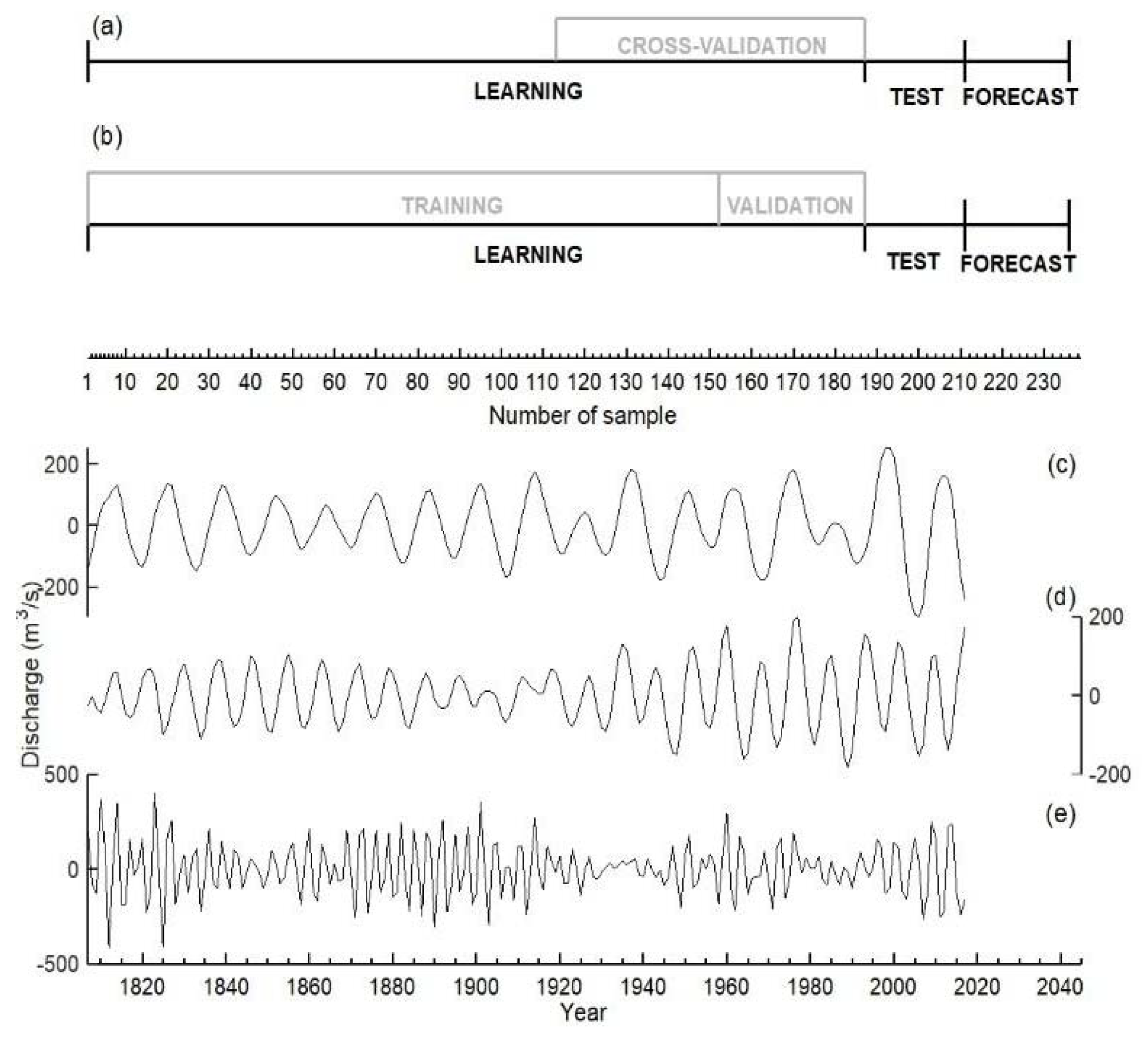
The prediction methodology builds on the AR-NN approach originally developed by Alessio et al. [10] and applied to the foraminiferal δ18O time series [28,29]. The idea is that a reliable prediction of the process underlying a time series can be obtained if the forecasting methods are applied not on the original record, but separately on its statistically significant variability modes. Such modes consist of the deterministic, and therefore predictable, part of the signal and can be detected using reliable spectral analysis methods. The advantages of this procedure are based on (i) the zeroing of the noise level (i.e., the removal of random and unpredictable components of the record) and (ii) the possibility to adjust the prediction algorithms to best fit the specific time scale of each considered variability mode [30]. Predictions are performed with two different algorithms, namely autoregressive models and feed-forward neural networks. Both methods rely on parameters evaluated through a training procedure, applied to the longest portion of the time series called the learning section (time interval 1807–1992). The performance of both methods is quantified comparing predictions with the observed data over the last 25 years, representing the test section. The choice of fixing the test section over the last portion of the time series relies on the fact that the significant components detected in the record could change their amplitude and phase over the time interval. In fact, the singular spectrum analysis (SSA) method we adopt is particularly efficient in detecting changes in the behavior of the oscillatory components inside a climate record, usually due to long-term trends in the climate system. In order to verify if our training algorithms would be able to capture properly such variability, we decide to focus the quantification of the prediction skill over the last portion of the time interval. Finally, we select the best models to forecast Po discharges for 25 years in the future, namely the period 2018–2042 (forecast section). The schematic diagram of this procedure is shown in Figure 2a,b. Both AR and NN algorithms are applied to each SSA–reconstructed component (RC) and the final forecast is obtained as the sum of the individual predictions.
The basic steps of the procedure we use to perform statistical predictions are reported in the following, while further details about the algorithms can be found in the Appendix A, Appendix B and Appendix C.

2.2.1. Detection of Deterministic Components of the Time Series

Several advanced spectral analysis methods could be used to detect the significant variability modes inside the considered climatic record. In this case, we apply the singular spectrum analysis (SSA; [31,32]), a technique designed to extract information from short and relatively noisy time series. It provides data-adaptive filters that separate the time series into components that are statistically independent and can be classified as oscillatory patterns or noise. Both the amplitude and phase of the oscillation can be modulated through time. In order to reliably identify the trend and oscillations in a series, the Monte Carlo method (MC-SSA) is used [33,34], assuming a model for the analyzed time series (null hypothesis) and determining the parameters using a maximum-likelihood criterion. More details about this method are reported in Appendix A.

2.2.2. AR Method

The AR method assumes that the output variable depends linearly on its MAR previous values, where MAR is the model order. We chose the order a posteriori using goodness-of-fit criteria to allow for a selection of the simplest possible model, i.e., the model with the fewest parameters that adequately describes the observations [35]. We use the final prediction error (FPE; [36]) and the Akaike information criterion (AIC; [37]) as estimators: the best order is the one that minimizes the values of both FPE and AIC. According to this procedure, the obtained results are: MAR,12yr = 16, MAR,8yr = 15 and MAR,3yr = 31. The AR model coefficients were computed with the Burg’s algorithm [38] over the learning section (Figure 2a) and the predictions are obtained by applying an iterative one-step-ahead procedure in the test and forecast sections. In order to quantify the prediction errors, we consider a section including the last 75 points of the time series (so-called cross-validation subsection, Figure 2a) corresponding to three times the value of the maximum lead time LMAX = 25 (25 years). The same procedure for the prediction error estimate is applied for both the hindcasts in the test section and the forecast in the forecast section. More details can be found in Appendix B.

2.2.3. NN Method

In the NN approach, we use feed-forward neural networks [39,40], fed by a delay line at the input, which presents to the input layer of the network progressively delayed versions of the input signal (formed by I elements), up to some maximum delay (lag). The net output is a single value and the predictions are obtained with an iterative, one-step-into-the-future procedure, as done for the AR prediction. Compared to the AR approach, in which all data in the learning section were used to evaluate the parameters of the model, here this section is further divided into training set (153 years) and validation set (33 years), as shown in Figure 2b. The parameter ranges of the NN architecture, namely the length I of the input vector and the numbers H1 and H2 of neurons in the hidden layers, are specifically evaluated for each component. A neural network with only one hidden layer was selected for the decadal component, while the other variability modes were predicted using two hidden layers. This difference is due to the fact that a very simple architecture is needed to obtain reliable and stable predictions for the 12-year component, which is the component with the longest period. The input vector length varies between 6 and 24 datasets, while the hidden layers contain 3–5 neurons. The NN predictions are obtained using the MATLAB Neural Network Toolbox. Further details are provided in Appendix C.

2.3. Metrics for Forecast Skill and Robustness

We evaluate our predictions’ performance in the test section using the RMSE calculated for progressively longer prediction intervals along the test section. Specifically, RMSE is calculated for each lead time as
RMSE ( l ) = 1 l i = 1 l ( y i p i ) 2
where l is the lead time (l = 1…L, with L = 25 in our analysis), yi is the value of the SSA component at the time i and pi is the corresponding predicted value. We compare RMSE values obtained from our AR and NN forecasts with those obtained from a persistence model. The persistence forecast assumes that future conditions will be the same as past conditions and is commonly used as a benchmark for decadal climate forecasts [41]. Specifically, we assume as a null hypothesis that in the next 25 years the discharge values (the denoised component) would remain constant and equal to the average value over the entire period covered by the record.
In order to quantitatively compare the AR and NN forecast skill, we evaluate several indices usually applied in hydrological studies (see e.g., [42]) to compare the hindcasts to the observed denoised discharge record in the test section. Besides the Pearson’s correlation coefficient, considered inappropriate for hydrological studies [43], we report the coefficient of efficiency (CE) and the Persistence Index (PI).
The coefficient of efficiency, also defined as the Nash–Sutcliffe coefficient [44], is defined as follows:
CE = 1 i = 1 L ( y i p i ) 2 i = 1 L ( y i y M ) 2
where yM is the average value of the denoised discharge record. When CE ~ 1 it means that the predictions match quite perfectly the observed data, while CE ~ 0 implies that predictions are as accurate as the mean of the observed data and, finally, CE < 0 is obtained when the residual variance (described by the numerator), is larger than the data variance (the denominator).
The definition of the Persistence Index is almost equal to that of CE, except for the fact that it involves the last known discharge value instead of the average value:
PI = 1 i = 1 L ( y i p i ) 2 i = 1 L ( y i y i 1 ) 2
Additionally, in this case, PI = 1 implies a perfect match between predicted and observed data and it is useful for its sensitiveness to possible lag effects affecting the predictions [45].
The robustness of the forecasts at each time step i is quantified through a compatibility test based on the standardized difference (D) between the predictions obtained with AR and NN methods. The forecasted values are defined as robust if Di ≤ 1, namely when the difference is compatible with 0 in 1σ range.
D i = | f i , A R f i , N N | σ i , A R 2 + σ i , N N 2
where fi,AR and fi,nn are the forecasted values at the time step i for the AR and NN methods, respectively, and σi,AR and σi,NN the associated uncertainties.

2.4. Drought Severity Quantification

In order to quantitatively estimate the severity of forecasted drought events, we use the standardized precipitation index (SPI, [46]). The SPI allows quantifying the precipitation deficit (in this case low-discharge values) for multiple time scales. We evaluate the SPI time series using the SSA-denoised discharge time series together with the 25 years forecasted with the AR method. We consider 5- and 10-year time scales in this analysis. A gamma probability density function is fitted to the empirical distribution of discharge values for the two timescales. Then, the probability of any discharge data point is calculated and used along with an estimate of the inverse normal distribution to calculate the discharge deviation for a normally distributed probability density with a mean of zero and standard deviation of unity. Drought is defined when SPI becomes −1.0 or less. The beginning of this drought is then defined as when the SPI first went negative, while the end does not occur until the SPI goes back to positive. Extreme droughts are characterized by values of the SPI < −2, while if −2 < SPI < −1 they are defined as moderate.

3. Results

3.1. Po River Spectral Analysis

We performed the SSA with a fairly wide range of window widths M, from 60 to 100 points, corresponding to the time windows W = M·Δt ranging from 60 to 100 years (Δt = 1 y). We consider only components significant at the 99% confidence level. According to the Monte Carlo test, the statistically significant part of the Po series is given by the first 14 empirical orthogonal functions (EOFs) accounting for roughly 40% of the total variance of the series. The error bars in Figure 3a bracket 99% of the eigenvalues of 10,000 surrogate series generated by a model that superposes EOFs 1−14 onto a red-noise process; the significant eigenvalues are those that lie outside the error bars (at 99% c.l.).
The significant components (EOFs 1−14) correspond to periods on the interannual and decadal scale (Figure 3b) estimated using the maximum entropy method. The corresponding reconstructed components (RCs) are shown in Figure 2c–e and have dominant periods (variances) of about 12.2 y (10.4%), 8 y (7.7%) and 3.3 y (20.5%). The SSA spectrum is dominated by a decadal component (EOFs 1,2,5), as discussed in previous works [6,15]. Nevertheless, most of the variance associated with the significant components is represented by the interannual oscillation because of the larger frequency band represented by this component with respect to the decadal one.

3.2. Hindcasts for the Last 25 Years

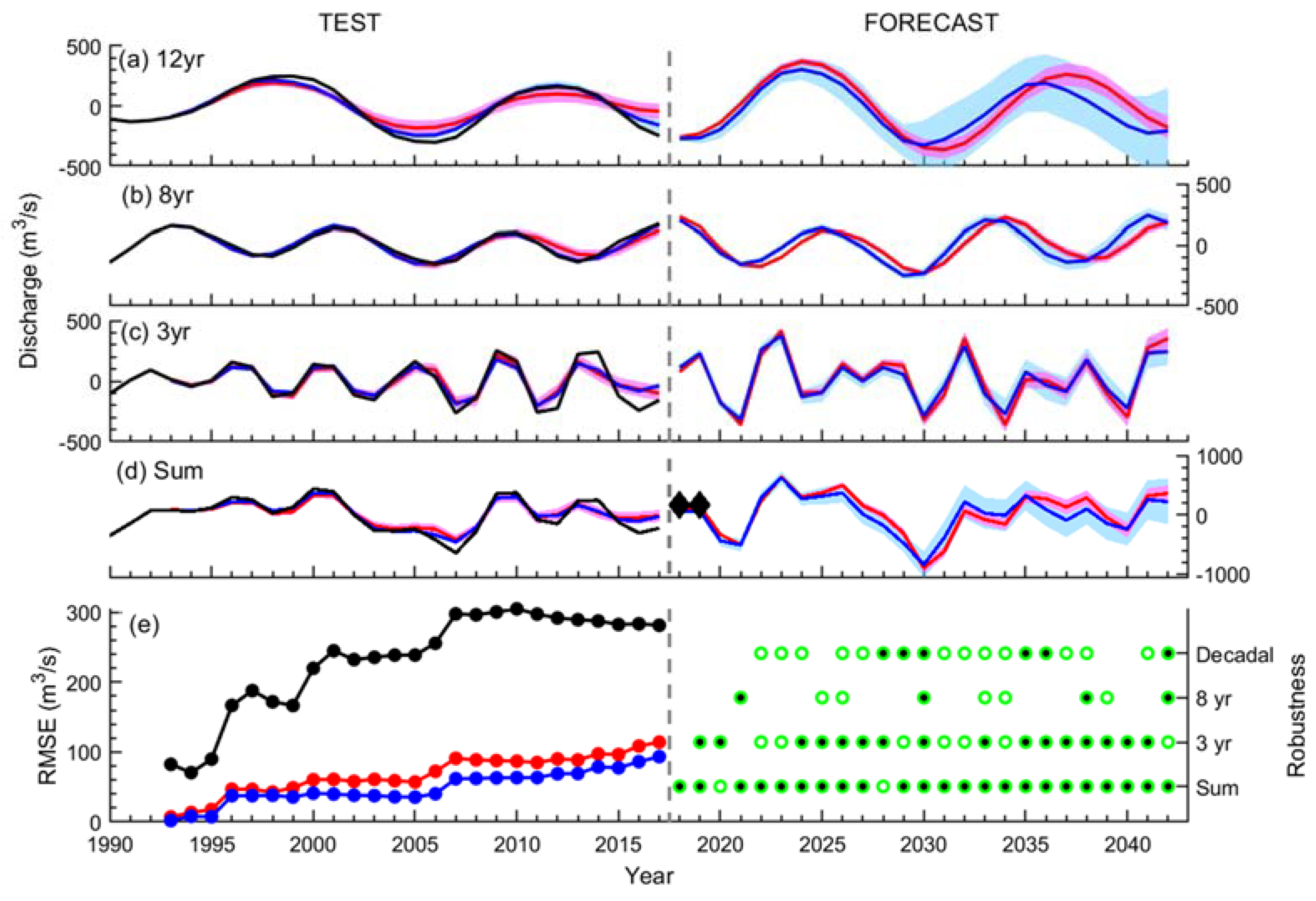
In order to quantify the performance of the applied prediction algorithms, we evaluate the hindcasts over a time interval corresponding to the test section consisting of the last 25 years of the time series (1993−2017). In this way, we can evaluate the hindcast over a time interval with the same length as the forecast. The single-component predictions obtained with the AR (red line) and NN (blue line) models are shown in the left column of Figure 4a–c together with the observed SSA–RCs (black line); their sum is shown in Figure 4d. Both methods perform similarly well in predicting the phase of the decadal component (Figure 4a), whereas the NN method surpasses the AR method concerning the prediction of the amplitude of this oscillation. Concerning the eight-year component, both methods skillfully predict both amplitude and phase of the observed data (Figure 4c). The AR prediction is affected by a one-year lag in the last cycle, which nonetheless corresponds to the temporal resolution of the series. Both results are in good agreement with the observed data concerning the interannual component, again with some exception for the last cycle (Figure 4c).
In order to quantify the prediction skill of our methods, we evaluate the RMSE between the denoised discharge signal and the correspondent hindcast for progressively longer prediction intervals (Figure 4e). We compare the results with that obtained with a persistence model (in this case quantified as the average value of the denoised signal), which assumes that future conditions will be the same as past conditions and is commonly used as a benchmark for decadal climate forecasts (see e.g., [41]). Results demonstrate that our forecasts largely beat the persistence forecast on all prediction intervals.
In Table 1, the values of the performance indices r, CE and PI, evaluated between the AR and NN predictions (red and blue curves in Figure 4d) and the denoised discharge signal (black curve in Figure 4d), are reported. Both methods show a highly significant correlation with the observed denoised data. The performance of the NN method results to be slightly higher with respect to that associated with the AR method, considering the CE and PI indices. In particular, PI demonstrates that AR models are more vulnerable to lag effects with respect to the NN one, even if it shows a PI value significantly higher than 0.

3.3. Forecast for the Next 25 Years

Figure 4 (right column) displays the forecasts for the time interval 2018–2042 obtained by the AR method (red curve) and by the NN method (blue curve) with the corresponding error bands. Figure 4a–c shows the forecast of the three observed SSA–RCs; Figure 4d shows their sum. The results obtained from both methods are statistically consistent, meaning that they overlap considering the error bands. Thus, two separate prediction algorithms provide consistent forecasts, which reinforces the reliability of the results. Concerning the 12-year and 8-year components, the agreement is remarkable concerning the amplitude. Note that the one-year lag between the NN and the AR forecasts detectable in Figure 4d is comparable with the series temporal resolution.
We highlight the following aspects of the forecast: 2020 would probably be a year characterized by a low annual average discharge value; then a period characterized by high discharge values, possibly associated with flood events, is expected to take place around 2023–2026. This is followed by a remarkable decrease in the late 2020s, which results in a large drought episode in the late 2020s/early 2030s; around 2032, the discharge values should return around the mean value of the total discharge record and no further extreme flood or drought event is predicted until the end of the forecast period.
In order to quantitatively assess the agreement of our forecasts, we evaluate the standardized difference (Di) between the forecasts obtained with AR and NN methods for each time step i. When DI ≤ 1, the twofold forecasts are defined to be robust. Figure 4e (right column) illustrates the result of the compatibility test. The total forecast shows overall robustness between both methods (except for two prediction years), thus confirming the strength of this twofold methodology. Considering the single components, the decadal and eight-year components result to be robust only for a few years. However, the decadal component predictions are compatible in the 2σ range (DI ≤ 2) over almost the entire forecasted period. On the contrary, the eight-year predictions are scarcely compatible, because of the phase lag affecting the AR method.
Black diamonds in Figure 4d represent the values of the SSA components obtained analyzing the record including the 2018–2019 period. A gap-filling procedure was applied to the monthly series of discharge data in order to estimate the missing data for the period July–October 2018, using the autoregressive model which minimizes the AIC over the remaining samples [36,47]. The observations are embedded within the forecast range, confirming the robustness of our results.
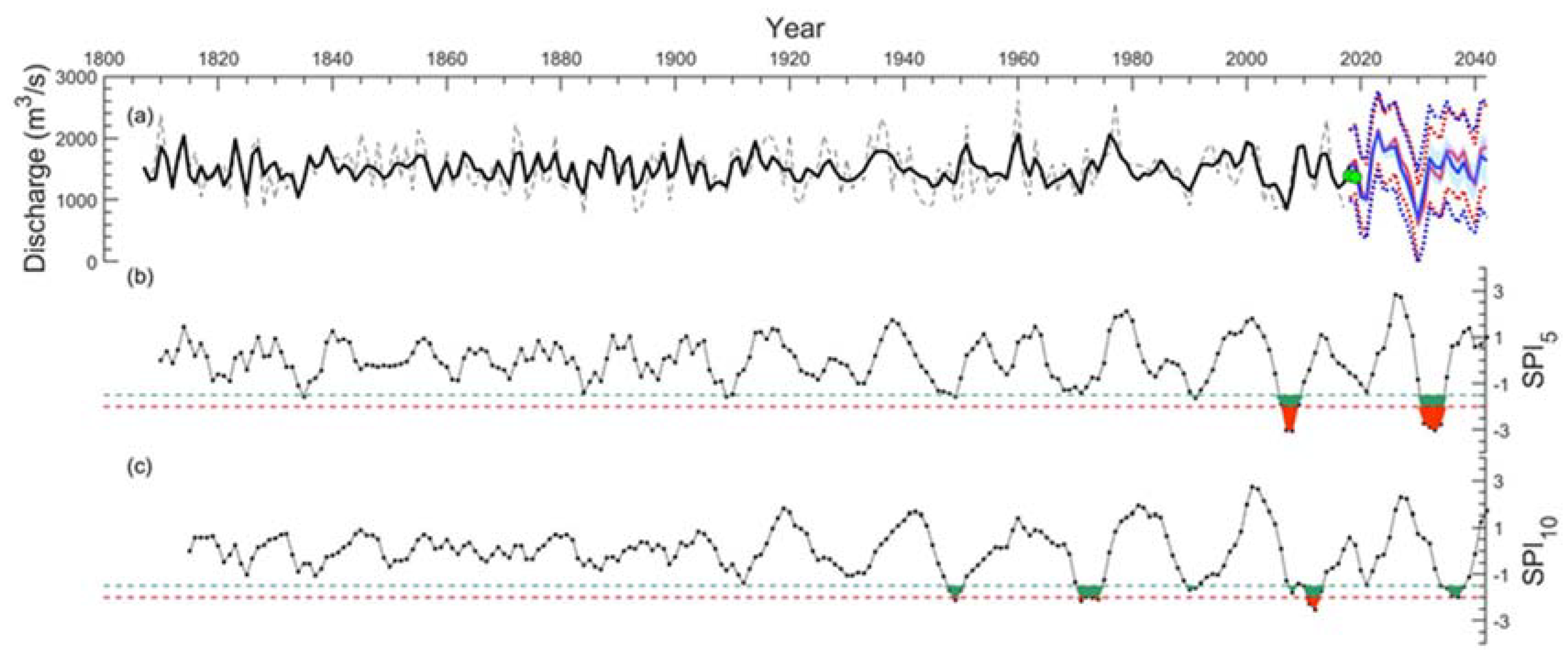
Figure 5a puts the total forecast for the next 25 years within the context of Po River discharge variability over the last two centuries. This figure allows appreciating that the forecasted wet-to-dry transition of nearly 800 m3/s between 2027 and 2030 is quite abrupt. Moreover, the forecasted drought in the late 2020s/early 2030s is expected to be of the same amplitude, or even more dramatic, than the droughts observed starting from 2003, a year characterized by the reduction of water flows of about 50–75% due to scarce precipitation in spring and high temperatures, over the seasonal average [48]. Since the statistical methods are applied to the denoised part of the discharge signal, they could explain the future variability of only ~40% of the total record. In order to provide a variability range effective for the total annual discharge, we add to the uncertainties associated with AR and NN predictions also the contribution of residuals, namely the random and unpredictable part of the discharge record. In Figure 5a, the total prediction bands are represented by the dotted red and blue curves. The contribution of residuals was evaluated as 95% c.l. of their cumulative distribution. Therefore, in this case, we can compare the raw discharge data for the period 2018–2019 with our predictions (green dots).

3.4. Evaluation of Drought Severity

Our forecasts indicate that in the next 25 years two low-discharge periods may occur. The first one is expected to verify in 2020. The second one is forecasted as prolonged dry phase over Northern Italy in the late 2020s/early 2030s, sharply following a ~5-year long wet phase in the early to mid-2020s (Figure 4). The severity of the predicted drought is comparable, or even exceeds, that of the mid-2000s. For a quantitative estimation of the drought severity, we calculate the SPI from the denoised Po River discharge series including the 25-year forecast obtained with the AR method (Figure 5a) for time scales of five years (SPI5, Figure 5b) and 10 years (SPI10, Figure 5c). Similar results are obtained with the NN method (not shown).
SPI5 reveals that the Po River experienced an increasing frequency of multiannual droughts in the course of the last centuries: only a moderate drought episode is detected during the 19th century (in the 1830s), whereas the 20th century is characterized by several moderate events (in the 1910s, 1940s, 1980s). The drought event in the first decade of this millennium (around 2003) is the only minimum classified as extreme according to the SPI5. The drought predicted in the late 2020s/early 2030s is extreme as well, following the historical tendency of increasing frequency and magnitude of multiannual droughts.
SPI10 indicates neither moderate nor extreme decadal droughts during the 19th century. Two events are classified as extreme during the 20th century (in the 1940s and 1960s) and one as moderate (in the 1980s). The minimum around 2003 ranks as extreme, whereas the forecasted drought in the late 2020s/early 2030s ranks as moderate.
Both SPI5 and SPI10 reveal that the intensity of the drought event in 2020 may be neither moderate nor extreme. Our forecasts thus support the intermittent occurrence of moderate/extreme decadal droughts over Northern Italy paced at intervals of about 20 years as observed in the past 60 years.

4. Discussion

4.1. Rainfall vs. Runoff Processes

Po River discharge predictions provide a statistical description of the near-future evolution of hydroclimate variability over Northern Italy. Interannual and decadal variations in Po discharges largely reflect variations in the amount of regional precipitation, as clearly evidenced by the comparison between Po discharges and the total annual precipitation from the HISTALP dataset over its basin (Figure 1b). The two records agree over the entire observational period (r = 0.75, p < 10−5) except for the first decade of this millennium, when strong annual precipitation contrasts with low discharges. This discrepancy seems to trace back to the quality of the HISTALP data in this period, as the E-OBS dataset provides precipitation values in the same period that are consistent with the discharge record. Even if discharges are determined both by direct precipitation and snow melting—besides evapotranspiration and runoff processes—no apparent correlation is detectable between annual discharge and near-surface air temperature recorded over neither the whole river basin nor the Alpine region (not shown). Therefore, if we consider discharge measurements close to the river mouth, annual precipitation variability dominates over temperature changes.
Spectral analysis on the updated Po River discharge record confirms previous results. SSA detected the same significant components on interannual, 8.2-, 12.9- and 19.2-year periods detected by wavelet analysis on the 1831–2003 monthly time series [5,14], even if in this case SSA merged variability modes with periods greater than 10 years into a unique component. The SSA method was also applied to the annual discharge record by Taricco et al. [6], over the period 1807–2006. In that case, the eight-year component was not detected, its significance being at a lower confidence level with respect to the reference chosen in that analysis (99%). The detected periodicities in Po discharge records correspond to those associated with variability modes already identified in other climatic records, thus indicating that our predictions could provide precious information related to the evolution of large-scale climatic patterns. In fact, significant peaks at about 3 y were detected in the autumn spectra of the Scandinavian pattern (SCA; [49]) and East Atlantic/Western Russian (EAWR; [50]) pattern, respectively [47]. The eight-year component dominates the power spectrum of the NAO index time series [14]. Finally, the decadal component is the most important variability mode characterizing the discharge records of the main European rivers [15].

4.2. Methodological Aspects

Our approach fully relies on a statistical description of the discharge process detectable in the available discharge time series alone, i.e., it does not need explanatory variables. It has, therefore, general applicability, pending that enough observational data are available to train the models. Until progress in downscaling of decadal climate predictions with numerical models [12] allows for a direct quantitative comparative assessment of forecast skills. we foresee the advantage that our approach avoids biases and uncertainties inherent in numerical dynamical climate models used in decadal climate predictions (e.g., [8]). The application of SSA in the data preprocessing phase allows the removal of noise, decomposing the series into simple components. This procedure improves the forecasting ability of the models [51] as also demonstrated in previous hydrologic studies (e.g., [42,52]).
The length of the testing and forecast period (both 25 years), which yields a ratio between testing and learning intervals of roughly 90/10, corresponds to about twice the periodicity of the longest component to be predicted. Further enlarging the testing interval, at expenses of the learning interval, leads, for the decadal component only, to noticeable degradation of the forecast skills in the testing phase and loss of the periodic signal in the forecasting phase (not shown). Our choice is therefore an attempt to balance learning/testing strategy with the specific characteristics of the dataset at hand and a sufficiently long forecast horizon. The occurrence of periods where the AR and NN forecasts significantly differ, even in the early portion of the prediction, supports the conclusion that both forecasts are not overconstrained and emphasizes the robustness of the predicted drought in the late 2020s/early 2030s.
In our application, the NN algorithm works on subsequent subsections for the training and validation procedure, but we also tested an alternative approach where the data are randomly divided between training and validation sets. The randomization destroys the autocorrelation of the data, but the alternative approach yields no detectable change in neither the test nor the forecast outcome, except for the decadal component (for which forecasts overlap anyway within associated uncertainties, not shown), which emerges again as the most critical element in our prediction.

4.3. Drought Severity and Attribution

Our analysis indicates that during the last two centuries Northern Italy evolved from a relatively stable and quiet 19th-century regime, with only one decadal drought episode identified in the 1830s, to a 20th-century regime characterized by recurrent decadal periods of low discharges and, most recently, to a significant intensification of interannual droughts culminated in the extreme events of the late 20th and early 21st centuries. According to the same analysis, the predicted discharge minimum in the late 2020s/early 2030s could have comparable, if not higher, severity as the extreme drought episode in the early-2000s. Our prediction sheds light on important aspects regarding trends in drought statistics for Northern Italy. Drought statistics will continue to strengthen progressively as observed in the recent past for multiannual time scales, whereas for a decadal time scale such strengthening appears more evanescent. Attribution of such tendencies is to be investigated in a future study; nevertheless, we propose here a few elements of discussion.
The evidence that precipitation is the dominant source of historical discharge variability (Section 4.1) builds confidence in the stability of the discharge process, hence on the learning and ultimately on the forecast. The consequent hypothesis that the predicted evolution reflects the continuation, in the upcoming decades, of local natural hydroclimatic variability is further supported by paleoclimatic evidence of highly significant decadal variability of Po River discharges persisting over the last two millennia [6] and by the temporally persistent spatial patterns detected in proxy-based hydroclimate reconstructions across the Mediterranean region during the past 12 centuries [53]. The hypothesis of a natural origin of the predicted evolution is also justified by the identification of significant volcanic and solar signals in North Atlantic/European regional climates [5] and supported by recent advances in the understanding of mechanisms of volcanically and solar forced decadal climate variability [8].
However, external disturbances that are not part of the historical functioning of the system are not accounted for in our prediction strategy, and would thus require an ad hoc estimation beyond the statistical approach. Reliable quantification of near-future temperature and precipitation changes in this region remains currently unavailable (e.g., [9,53]). We nonetheless speculate that warmer temperatures, especially in the dry summer season, would contribute to worsening North Italian droughts through strengthened evaporation and evapotranspiration processes. Indeed, a simple long-term water budget for the Po River basin indicates that only about 60% of precipitation is converted to discharge, the rest being mostly lost through evapotranspiration [5].

4.4. Broader Climatic and Socioeconomic Implications

The strong correlation between the historical discharge time series of the Po River and of minor Alpine rivers suggests that the predicted late 2020s/early 2030s drought could extend beyond the Po basin alone. The predicted North Italian drought could have profound influences on water stratification of the Eastern Mediterranean: a weak river discharge can favor the formation of particularly salty North Adriatic deep water [54]. In the long term, such modifications can significantly affect the large-scale deep oceanic circulation in the Eastern Mediterranean basin [55,56]. The oceanic response will also crucially depend on the basin’s thermal state, as warmer temperatures would contrast the buoyancy effects of increased salinity. How these changes induced in the coupled regional ocean-atmosphere system will reverberate on North Italian hydroclimate remains to be understood.
Finally, the forecasted Po River discharge minimum could have substantial societal and economic effects. Approximately 16 million people live in the Po basin and about 40% of the gross domestic product of Italy is made in this region. In particular, 35% of the Italian agricultural production comes from this area [13,57] and the drought forecasted for the late 2020s/early 2030s could therefore strongly impact this sector.

5. Conclusions

We presented a twofold statistical approach for a robust interannual-to-decadal prediction of midsize basin river discharges for the Euro-Mediterranean region, using the North Italian Po River as a case study. The approach consists in the application of two separate methods, an autoregressive model and a feed-forward neural network algorithm, fed with the significant components of the discharge time series extracted by Singular Spectrum Analysis. The two methods yield a convergent decadal forecast. A fundamental aspect characterizing this methodology lies in the careful preprocessing of the time series for noise removal and separation of the significant variability modes characterizing the record according to their timescales. This study paves the way to a broader application of statistical decadal prediction methods in the field of hydrology and climatology, particularly in regions where variability is dominated by persistent interannual and decadal fluctuations and availability of long observational records allows their reliable quantification.
The 25-year forecasts obtained with both methods consistently indicate in particular that a discharge maximum is expected around 2023–2026, followed by a minimum in the late 2020s/early 2030s. The forecasts confirm the secular trend of increasing severity of Po River drought events in terms of both amplitude and duration. This drought is in line with the secular trend of increasing the severity of decadal drought events observed in the Po River time series. We can thus speculate that this long-term trend may continue beyond the decadal forecast horizon of this study.

Author Contributions

C.T., S.A. and S.R. conceived the initial research idea. S.R., C.T. and D.Z. developed the research. S.R. and S.A. performed the analyses. All authors contributed to the discussion and the manuscript writing. All authors have read and agreed to the published version of the manuscript.

Funding

This work has been supported by the Fondazione CRT (project title: Variabilità idrologica del bacino padano: eventi alluvionali estremi e periodi di siccità dall’epoca romana ad oggi).

Acknowledgments

Updated Po River discharge data were obtained through Dext3r.

Conflicts of Interest

The authors declare no conflicts of interest. The funders had no role in the design of the study; in the collection, analyses, or interpretation of data; in the writing of the manuscript, or in the decision to publish the results.

Appendix A

Singular Spectrum Analysis (SSA)

The SSA methodology involves three basic steps: (a) embedding a time series of length N in a vector space of proper dimension M; (b) computing the M x M lag-covariance matrix CD of the data (we used the approach by Vautard and Ghil [58]); and (c) diagonalizing CD, thus evaluating ΛD = EDTCDED, where ΛD = diag(λ123,…λM), with λ1 > λ2 > λ3 > … > λM > 0, and ED is the M x M matrix having the corresponding eigenvectors Ek, k = 1,M as its columns. For each Ek we construct the time series, of length N – M + 1, called the k-th principal component (PC); this PC represents the projection of the original time series on the eigenvector Ek (also called empirical orthogonal function (EOF)). Each eigenvalue λk gives the variance of the corresponding PC; its square root is called singular value. Given a subset of eigenvalues, it is possible to extract time series of length N by combining the corresponding PCs; these time series are called reconstructed components (RCs) and capture the variability associated with the eigenvalues of interest. In order to reliably identify the trend and oscillations in a series, the Monte Carlo method (MC-SSA) is used [33]. In this approach, we assume a model for the analyzed time series (null hypothesis) and we determine the parameters using a maximum-likelihood criterion. Then a Monte Carlo ensemble of surrogate time series (size 10,000) is generated from the model and SSA is applied to data and surrogates (EOFs of the null hypothesis basis are used), in order to test whether it is possible to distinguish the series from the ensemble. Since a large class of geophysical processes generates series with larger power at lower frequencies, we assume autoregressive lag-1 noise in evaluating evidence for trend and oscillations. This is done to avoid overestimating the system predictability, by underestimating the amplitude of the stochastic component of the time series. SSA is particularly useful for climatic time series, which are most often short and noisy. For the calculations, we used the freeware SSA-MTM Toolkit [59,60].

Appendix B

Autoregressive Model Method

This method for statistical climate predictions is based on AR models, as introduced by Keppenne and Ghil [51,61] and further described in Ghil et al. [31]; it is also implemented in the kSpectra Toolkit [62]. The algorithm for this procedure consists in the steps described in the following.
  • Selection of the best order of the AR method. The AR method turns out to be most reliable and robust when the order MAR of the autoregressive model is not too large with respect to the length N of the time series, since the variance of the AR-coefficient estimates increases with the order. For this analysis, the choice of a suitable AR order is done a posteriori using goodness-of-fit criteria [35], namely the final prediction error (FPE; [36]) and the Akaike information criterion (AIC; [37]). We perform the predictions over the test section using a wide range of values of the AR model (between 1 and 60) and calculate both AIC and FPE values. The value of MAR which minimizes these indices is selected to perform the forecasts.
  • Evaluation of the AR model coefficients. The values of the MAR coefficients of model are evaluated with Burg’s algorithm [38] applied to the learning section.
  • Quantification of the prediction error. In order to quantify the uncertainty associated with this method, we perform 25-year predictions over different portions of this time interval (namely the cross-validation section, Figure 2a). More specifically, we repeat the procedure of the previous point varying the length of the learning section. In this way we obtain an ensemble of 25-year-predictions translated in time. By evaluating the root-mean-square-error between the predicted and original data as a function of the lead time (RMSE(l)) we obtain the uncertainty associated with the predictions. A useful scheme describing this procedure can be found in Alessio et al. [10].

Appendix C

Neural Network Method

For this multistep-ahead prediction we use feed-forward neural network (FFNN) which are more suitable in case of relatively short time series. Instead of using a single network architecture for each series, we initialize and train a whole set of feed-forward NNs that all had a single output value and a maximum of two hidden layers, with varying number of input data and neurons in the hidden layers. In this way, the network architecture is chosen a posteriori, on the basis of the algorithm performance. The basics steps of this procedure are:
  • Partition of the learning section. While in the AR method all the data in the learning section are used to evaluate the coefficients of the model, in this case this, section is divided into two subsections: training (82% of the data in the learning section) and validation (18%). The partition can consist of continuous blocks, as shown in Figure 2b, or also in a random division of the data into the two subsets.
  • Training of the network. The training set is used to compute the error gradient and update the weights and biases according to the Levenberg–Marquardt algorithm [63,64]. The validation set serves to assess the predictive skills of the NN being trained. More specifically, the error on the validation set—namely the mean squared error between predicted and observed data—is monitored during the training process and normally decreases during the initial phase of training, as does the training set error. When the network begins to overfit the data, the error on the validation set typically begins to rise. Thus, the final network weights and biases are those yielding the minimum error on the validation set. The parameter ranges of the NN architecture, namely the length I of the input vector and the numbers H1 and H2 of neurons in the hidden layers, are specifically evaluated for each component. The transfer functions used to evaluate the neuron scalar output are the sigmoid hyperbolic-tangent function for the hidden layers and the linear function for the output one.
  • Prediction and quantification of the error. Each trained network is used to forecast the component in the test section, and the corresponding RMSE is calculated between predicted and observed data. Then, among all the values of I, H1 and H2, the network architecture that best reproduces the samples in the test section is chosen. The trained network is finally used for the predictions over the forecast section. Since the training process depends upon the random choice of the initial guesses for weights and biases, the procedure described above is repeated 100 times for each component, thus yielding 100 predictions. Then, the average of all the predictions in both the test and the forecasting section is evaluated, after discarding potential anomalous scenarios. Error bands associated with the predictions correspond to one standard deviation, while the standard error of the mean is used as the uncertainty associated with the average prediction.

References

  1. Hurrell, J.W. Decadal trends in the North Atlantic Oscillation: Regional temperatures and precipitation. Science 1995, 269, 676–678. [Google Scholar] [CrossRef] [Green Version]
  2. Giorgi, F. Climate change hot-spots. Geophys. Res. Lett. 2006, 33, L08707. [Google Scholar] [CrossRef]
  3. Gray, L.J.; Scaife, A.A.; Mitchell, D.M.; Osprey, S.; Ineson, S.; Hardiman, S.; Butchart, N.; Knight, J.; Sutton, R.; Kodera, K. A lagged response to the 11 year solar cycle in observed winter Atlantic/European weather patterns. J. Geophys. Res. Atmos. 2013, 118, 13405–13420. [Google Scholar] [CrossRef] [Green Version]
  4. Brunetti, M.; Maugeri, M.; Nanni, T.; Auer, I.; Böhm, R.; Schöner, W. Precipitation variability and changes in the greater Alpine region over the 1800–2003 period. J. Geophys. Res. Atmos. (1984–2012) 2006, 111. [Google Scholar] [CrossRef]
  5. Zanchettin, D.; Traverso, P.; Tomasino, M. Po River discharges: A preliminary analysis of a 200-year time series. Clim. Chang. 2008, 89, 411–433. [Google Scholar] [CrossRef]
  6. Taricco, C.; Alessio, S.; Rubinetti, S.; Zanchettin, D.; Cosoli, S.; Gačić, M.; Mancuso, S.; Rubino, A. Marine Sediments Remotely Unveil Long-Term Climatic Variability Over Northern Italy. Sci. Rep. 2015, 5. [Google Scholar] [CrossRef] [Green Version]
  7. Kirtman, B.; Power, S.B.; Adedoyin, A.J.; Boer, G.J.; Bojariu, R.; Camilloni, I.; Doblas-Reyes, F.; Fiore, A.M.; Kimoto, M.; Meehl, G.; et al. Near-term climate change: Projections and predictability. In Climate Change 2013 the Physical Science Basis: Working Group I Contribution to the Fifth Assessment Report of the Intergovernmental Panel on Climate Change; Cambridge University Press: Cambridge, UK, 2013; pp. 953–1028. [Google Scholar]
  8. Zanchettin, D. Aerosol and solar irradiance effects on decadal climate variability and predictability. Curr. Clim. Chang. Rep. 2017, 3, 150–162. [Google Scholar] [CrossRef]
  9. Xie, S.-P.; Deser, C.; Vecchi, G.A.; Collins, M.; Delworth, T.L.; Hall, A.; Hawkins, E.; Johnson, N.C.; Cassou, C.; Giannini, A.; et al. Towards predictive understanding of regional climate change. Nat. Clim. Chang. 2015, 5, 921–930. [Google Scholar] [CrossRef]
  10. Alessio, S.; Vivaldo, G.; Taricco, C.; Ghil, M. Natural variability and anthropogenic effects in a Central Mediterranean core. Clim. Past 2012, 8, 831–839. [Google Scholar] [CrossRef] [Green Version]
  11. Boer, G.J.; Smith, D.M.; Cassou, C.; Doblas-Reyes, F.; Danabasoglu, G.; Kirtman, B.; Kushnir, Y.; Kimoto, M.; Meehl, G.A.; Msadek, R.; et al. The decadal climate prediction project (DCPP) contribution to CMIP6. Geosci. Model. Dev. (Online) 2016, 9, 3751–3777. [Google Scholar] [CrossRef] [Green Version]
  12. Benestad, R.; Caron, L.-P.; Parding, K.; Iturbide, M.; Gutierrez Llorente, J.M.; Mezghani, A.; Doblas-Reyes, F.J. Using statistical downscaling to assess skill of decadal predictions. Tellus A Dyn. Meteorol. Oceanogr. 2019, 71, 1–19. [Google Scholar] [CrossRef] [Green Version]
  13. Po River Watershed Authority Caratteristiche del bacino del fiume Po e primo esame dell?impatto ambientale delle attività umane sulle risorse idriche. Period. Agency Rep. 2006.
  14. Zanchettin, D.; Rubino, A.; Traverso, P.; Tomasino, M. Impact of variations in solar activity on hydrological decadal patterns in northern Italy. J. Geophys. Res. Atmos. (1984–2012) 2008, 113, D12102. [Google Scholar] [CrossRef] [Green Version]
  15. Zanchettin, D.; Toniazzo, T.; Taricco, C.; Rubinetti, S.; Rubino, A.; Tartaglione, N. Atlantic origin of asynchronous European interdecadal hydroclimate variability. Sci. Rep. 2019, 9, 10998. [Google Scholar] [CrossRef] [PubMed] [Green Version]
  16. Tomasino, M.; Zanchettin, D.; Traverso, P. Long-range forecasts of River Po discharges based on predictable solar activity and a fuzzy neural network model. Hydrol. Sci. J. 2004, 49, 684. [Google Scholar] [CrossRef]
  17. Smith, D.M.; Scaife, A.A.; Eade, R.; Knight, J.R. Seasonal to decadal prediction of the winter North Atlantic Oscillation: Emerging capability and future prospects. Q. J. R. Meteorol. Soc. 2016, 142, 611–617. [Google Scholar] [CrossRef]
  18. Coppola, E.; Giorgi, F. An assessment of temperature and precipitation change projections over Italy from recent global and regional climate model simulations. Int. J. Climatol. A J. R. Meteorol. Soc. 2010, 30, 11–32. [Google Scholar] [CrossRef]
  19. Pawlowicz, R. M_Map: A Mapping Package for MATLAB. Version 1.4k. 2019. Available online: www.eoas.ubc.ca/~rich/map.html (accessed on 27 July 2019).
  20. Gorny, A. World Data Bank II General User GuideRep; Central Intelligence Agency: Washington, DC, USA, 1977.
  21. Soluri, E.; Woodson, V. World vector shoreline. Int. Hydrogr. Rev. 1990, 67, 27–35. [Google Scholar]
  22. Wessel, P.; Smith, W.H. A global, self-consistent, hierarchical, high-resolution shoreline database. J. Geophys. Res. 1996, 101, 8741–8743. [Google Scholar] [CrossRef] [Green Version]
  23. Amante, C.; Eakins, B. ETOPO1 1 Arc-minute global relief model: Procedures, data sources and analysis. NOAA Technical Memorandum NESDIS NGDC-24. Natl. Geophys. Data Cent. Noaa 2009, 10, V5C8276M. [Google Scholar]
  24. Auer, I.; Böhm, R.; Jurkovic, A.; Lipa, W.; Orlik, A.; Potzmann, R.; Schöner, W.; Ungersböck, M.; Matulla, C.; Briffa, K.; et al. HISTALP—historical instrumental climatological surface time series of the Greater Alpine Region. Int. J. Climatol. 2007, 27, 17–46. [Google Scholar] [CrossRef]
  25. Brunetti, M.; Lentini, G.; Maugeri, M.; Nanni, T.; Auer, I.; Boehm, R.; Schoener, W. Climate variability and change in the Greater Alpine Region over the last two centuries based on multi-variable analysis. Int. J. Climatol. 2009, 29, 2197–2225. [Google Scholar] [CrossRef]
  26. Efthymiadis, D.; Jones, P.D.; Briffa, K.R.; Auer, I.; Böhm, R.; Schöner, W.; Frei, C.; Schmidli, J. Construction of a 10-min-gridded precipitation data set for the Greater Alpine Region for 1800–2003. J. Geophys. Res. Atmos. 2006, 111, D01105. [Google Scholar] [CrossRef] [Green Version]
  27. Haylock, M.; Hofstra, N.; Klein Tank, A.; Klok, E.; Jones, P.; New, M. A European daily high-resolution gridded data set of surface temperature and precipitation for 1950–2006. J. Geophys. Res. Atmos. 2008, 113, D20119. [Google Scholar] [CrossRef] [Green Version]
  28. Taricco, C.; Ghil, M.; Alessio, S.; Vivaldo, G. Two millennia of climate variability in the Central Mediterranean. Clim. Past 2009, 5, 171–181. [Google Scholar] [CrossRef] [Green Version]
  29. Taricco, C.; Alessio, S.M.; Rubinetti, S.; Vivaldo, G.; Mancuso, S. A foraminiferal δ18O record covering the last 2,200 years. Sci. Data 2016, 3, 160042. [Google Scholar] [CrossRef] [Green Version]
  30. Penland, C.; Ghil, M.; Weickmann, K.M. Adaptive filtering and maximum entropy spectra with application to changes in atmospheric angular momentum. J. Geophys. Res. Atmos. 1991, 96, 22659–22671. [Google Scholar] [CrossRef]
  31. Ghil, M.; Allen, M.R.; Dettinger, M.D.; Ide, K.; Kondrashov, D.; Mann, M.E.; Robertson, A.W.; Saunders, A.; Tian, Y.; Varadi, F.; et al. Advanced Spectral Methods For Climatic Time Series. Rev. Geophys. 2002, 40, 1003–1043. [Google Scholar] [CrossRef] [Green Version]
  32. Ghil, M.; Taricco, C. Advanced spectral-analysis methods. In Past and Present Variability of the Solar-Terrestrial System: Measurement, Data Analysis and Theoretical Models; Castagnoli, G.C., Provenzale, A., Eds.; IOS Press: Amsterdam, The Netherlands, 1997; pp. 137–159. [Google Scholar]
  33. Allen, M.; Smith, L. Monte Carlo SSA: Detecting irregular oscillations in the presence of colored noise. J. Clim. 1996, 9, 3373–3404. [Google Scholar] [CrossRef]
  34. Groth, A.; Ghil, M. Monte Carlo singular spectrum analysis (SSA) revisited: Detecting oscillator clusters in multivariate datasets. J. Clim. 2015, 28, 7873–7893. [Google Scholar] [CrossRef] [Green Version]
  35. Alessio, S.M. Digital Signal Processing and Spectral Analysis for Scientists: Concepts and Applications; Springer International Publishing: Cham, Switzerland, 2015. [Google Scholar]
  36. Akaike, H. Statistical predictor identification. Ann. Inst. Stat. Math. 1970, 22, 203–217. [Google Scholar] [CrossRef]
  37. Akaike, H. A new look at the statistical model identification. IEEE Trans. Autom. Control. 1974, 19, 716–723. [Google Scholar] [CrossRef]
  38. Burg, J.P. Maximum entropy spectral analysis. In Proceedings of the 37th Annual International Meeting, Society of Exploration Geophysicists, Oklahoma City, OK, USA, 31 October 1967. [Google Scholar]
  39. Hagan, M.T.; Demuth, H.B.; Beale, M.H.; De Jesús, O. Neural Network Design; PWS publishing company: Boston, MA, USA, 1996. [Google Scholar]
  40. Haykin, S. Neural Networks: A Comprehensive Approach; Prentice Hall: Upper Saddle River, NJ, USA, 1999. [Google Scholar]
  41. Matei, D.; Pohlmann, H.; Jungclaus, J.; Müller, W.; Haak, H.; Marotzke, J. Two tales of initializing decadal climate prediction experiments with the ECHAM5/MPI-OM model. J. Clim. 2012, 25, 8502–8523. [Google Scholar] [CrossRef]
  42. Wu, C.; Chau, K.; Fan, C. Prediction of rainfall time series using modular artificial neural networks coupled with data-preprocessing techniques. J. Hydrol. 2010, 389, 146–167. [Google Scholar] [CrossRef] [Green Version]
  43. Legates, D.R.; McCabe, G.J., Jr. Evaluating the use of “goodness-of-fit” measures in hydrologic and hydroclimatic model validation. Water Resour. Res. 1999, 35, 233–241. [Google Scholar] [CrossRef]
  44. Nash, J.E.; Sutcliffe, J.V. River flow forecasting through conceptual models part I—A discussion of principles. J. Hydrol. 1970, 10, 282–290. [Google Scholar] [CrossRef]
  45. Kitanidis, P.K.; Bras, R.L. Real-time forecasting with a conceptual hydrologic model: 1. Analysis of uncertainty. Water Resour. Res. 1980, 16, 1025–1033. [Google Scholar] [CrossRef]
  46. McKee, T.B.; Doesken, N.J.; Kleist, J. The relationship of drought frequency and duration to time scales. In Proceedings of the 8th Conference on Applied Climatology, Boston, MA, USA, 17–22 January 1993; Volume 17, pp. 179–183. [Google Scholar]
  47. Orfanidis, S.J. Optimum Signal Processing: An Introduction; Collier Macmillan: New York, NY, USA, 1988. [Google Scholar]
  48. Musolino, D.; de Carli, A.; Massarutto, A. Evaluation of socio-economic impact of drought events: The case of Po river basin. Eur. Countrys. 2017, 9, 163–176. [Google Scholar] [CrossRef] [Green Version]
  49. Bueh, C.; Nakamura, H. Scandinavian pattern and its climatic impact. Q. J. R. Meteorol. Soc. 2007, 133, 2117–2131. [Google Scholar] [CrossRef]
  50. Krichak, S.O.; Alpert, P. Decadal trends in the east Atlantic–west Russia pattern and Mediterranean precipitation. Int. J. Climatol. 2005, 25, 183–192. [Google Scholar] [CrossRef]
  51. Keppenne, C.L.; Ghil, M. Adaptive filtering and prediction of noisy multivariate signals: An application to subannual variability in atmospheric angular momentum. Int. J. Bifurc. Chaos 1993, 3, 625–634. [Google Scholar] [CrossRef]
  52. Marques, C.; Ferreira, J.; Rocha, A.; Castanheira, J.; Melo-Gonçalves, P.; Vaz, N.; Dias, J. Singular spectrum analysis and forecasting of hydrological time series. Phys. Chem. Earth Parts A/B/C 2006, 31, 1172–1179. [Google Scholar] [CrossRef]
  53. Ljungqvist, F.C.; Krusic, P.J.; Sundqvist, H.S.; Zorita, E.; Brattström, G.; Frank, D. Northern Hemisphere hydroclimate variability over the past twelve centuries. Nature 2016, 532, 94–98. [Google Scholar] [CrossRef]
  54. Bensi, M.; Rubino, A.; Cardin, V.; Hainbucher, D.; Mancero-Mosquera, I. Structure and variability of the abyssal water masses in the Ionian Sea in the period 2003-2010. J. Geophys. Res. 2013, 118, 931–943. [Google Scholar] [CrossRef] [Green Version]
  55. Hainbucher, D.; Rubino, A.; Klein, B. Water mass characteristics in the deep layers of the western Ionian Basin observed during May 2003. Geophys. Res. Lett. 2006, 33, L05608. [Google Scholar] [CrossRef] [Green Version]
  56. Rubino, A.; Hainbucher, D. A large abrupt change in the abyssal water masses of the eastern Mediterranean. Geophys. Res. Lett. 2007, 34, L23607. [Google Scholar] [CrossRef] [Green Version]
  57. Bozzola, M.; Swanson, T. Policy implications of climate variability on agriculture: Water management in the Po river basin, Italy. Environ. Sci. Policy 2014, 43, 26–38. [Google Scholar] [CrossRef]
  58. Vautard, R.; Ghil, M. Singular spectrum analysis in nonlinear dynamics, with applications to paleoclimatic time series. Phys. D 1989, 35, 395–424. [Google Scholar] [CrossRef]
  59. Vautard, R.; Yiou, P.; Ghil, M. Singular-spectrum analysis: A toolkit for short, noisy chaotic signals. Phys. D 1992, 58, 95–126. [Google Scholar] [CrossRef]
  60. SSA-MTM Toolkit. Available online: http://research.atmos.ucla.edu/tcd/ssa/ (accessed on 14 June 2017).
  61. Keppenne, C.L.; Ghil, M. Adaptive filtering and prediction of the Southern Oscillation index. J. Geophys. Res. Atmos. 1992, 97, 20449–20454. [Google Scholar] [CrossRef] [Green Version]
  62. kSpectra Toolkit for Mac OS X! Available online: http://www.spectraworks.com/web/products.html (accessed on 6 May 2020).
  63. Hagan, M.T.; Menhaj, M.B. Training feedforward networks with the Marquardt algorithm. IEEE Trans. Neural Netw. 1994, 5, 989–993. [Google Scholar] [CrossRef] [PubMed]
  64. Rumelhart, D.; Hinton, G.; Williams, R. Learning Internal Representations by Error Propagation, Parallel Distributed Processing, Explorations in the Microstructure of Cognition, ed. DE Rumelhart and J. McClelland. Vol. 1. 1986. Biometrika 1986, 71, 599–607. [Google Scholar]
Figure 1. (a) Po River basin and location of the Pontelagoscuro gauge station (44°53’19.34’’ N, 11°36’29.60’’ E; red diamond). This map was obtained with MATLAB using the m_map package [19] and the GSHHG dataset for coastlines [20,21,22] and the ETOPO one [23] for elevation and bathymetry. The black rectangle represents the area over which total annual precipitations were evaluated over the Po plain (44–46° N, 7–12° E). (b) Comparison between annual Po discharges (black curve) and total annual precipitation (blue curve) over the Po basin using data from the HISTALP dataset. From the year 1950 onward, precipitation data from the E-OBS dataset (green curve in (b)) are also considered.
Atmosphere 11 00671 g001
Figure 2. (a,b) Schematic diagram of the sections in which the input data series were divided according to the prediction method selected. For both autoregressive (AR) and neural network (NN) models, the length of the learning, test and forecast sections are the same. Nevertheless, while the AR algorithm uses all the available data to evaluate the coefficients of the autoregressive model (a), the NN method requires that the learning section be further divided into training and validation subsections (b), as described in the text. Both methods were applied to evaluate the hindcasts over the test section in order to compare the predictions to the data included in the last portion of the time series. Finally, the forecasts for the next 25 years are evaluated for the forecast section. Uncertainties associated with AR forecasts were obtained performing 25-year predictions over different portions of this time interval (cross-validation subsection) and then evaluating the RMSE between the predicted and original data as a function of the lead time. (ce) Significant oscillatory components in the Po River discharge series, obtained with singular spectrum analysis (SSA): reconstructed components (RCs) 1–2,5 (~12-year period; (c)), 8–10 (~8-year period; (d)) and 3–4,6–7,11–14 (~3-year period; (e)).
Atmosphere 11 00671 g002
Figure 3. Spectral properties of the Po River discharge series. (a) Monte Carlo-SSA test performed using EOFs 1–14 and AR(1) as the null hypothesis model (window width W = 80 y and Monte Carlo ensemble size 10,000). The red dots mark the eigenvalues corresponding to the empirical orthogonal functions (EOFs) included in the null hypothesis. No excursions occur outside the 99% limits, indicating that the series is well explained by this model. The periods associated with the reconstructed components (RCs) are: ~12 y (RCs 1−2,5), ~8 y (RCs 8−10) and ~3 y (3−4, 6−7, 11−14). (b) Power spectrum obtained performing the spectral analysis of the sum of all the significant components of the Po discharge series, performed using the maximum entropy method (order 20, see [35] and references therein).
Atmosphere 11 00671 g003
Figure 4. (ad) Prediction (left column) and forecast (right column) results for the three components of the Po River discharges over the test (1993–2017) and the forecast (2018–2042) sections. In black, the RCs reconstructed by SSA are plotted, while in red the predictions obtained by the AR method and in blue those obtained by the NN method are shown with the associated error bands. All components are represented as zero-mean. Black diamonds in (d) represent the values of the SSA components obtained analyzing the record including the 2018–2019 period. This SSA analysis was applied using a window width w = 80 y and the significant components extracted are RCs 1−13,15−16. (e) Left column: progressive RMSE as a function of lead time evaluated for both the AR and NN methods (dotted red and blue curves, respectively) and for the persistence hypothesis (dotted black curve). The RMSE is evaluated between the denoised discharge time series (black curve in (d)) and the corresponding predictions. Right column: results of the compatibility test performed between the AR and NN forecasts for each time step. Black dots indicate when the predictions are robust, namely when their difference is compatible with 0 (in the 1σ range). Empty green dots indicate when the difference is null in the 2σ range.
Atmosphere 11 00671 g004
Figure 5. Standardized precipitation index (SPI) time series calculated for Po River discharge denoised series and the forecasted time period 2018–2042. (a) Po River discharges (dotted black curve) and corresponding denoised series (black curve) with the associated forecast obtained using the AR model (red curve) and the feed-forward neural network (FFNN) method (blue curve). Dotted blue and red curves represent the total uncertainty associated with the forecasts, considering also the contribution of the residuals. Green dots represent raw annual average discharge data for the period 2018–2019. (bc) Five-year and ten-year SPI time series. The horizontal lines individuate the thresholds for the categories of severity by [38], namely moderate (SPI = −1, green line) and extreme (SPI = −2, red line) droughts. The colored areas indicate periods when the Po River basin experienced moderate (green areas) and extreme (red areas) droughts.
Atmosphere 11 00671 g005
Table 1. Performance indices evaluated between the AR and NN total predictions and the sum of significant SSA components. The definition of the indices is reported in Section 2.3.
r (p-Value)CEPI
AR0.95 (<10−4) 0.840.79
NN0.96 (<10−3)0.890.86