All-Sky Imager Observations of the Latitudinal Extent and Zonal Motion of Magnetically Conjugate 630.0 nm Airglow Depletions

 ,
,
Abstract
1. Introduction
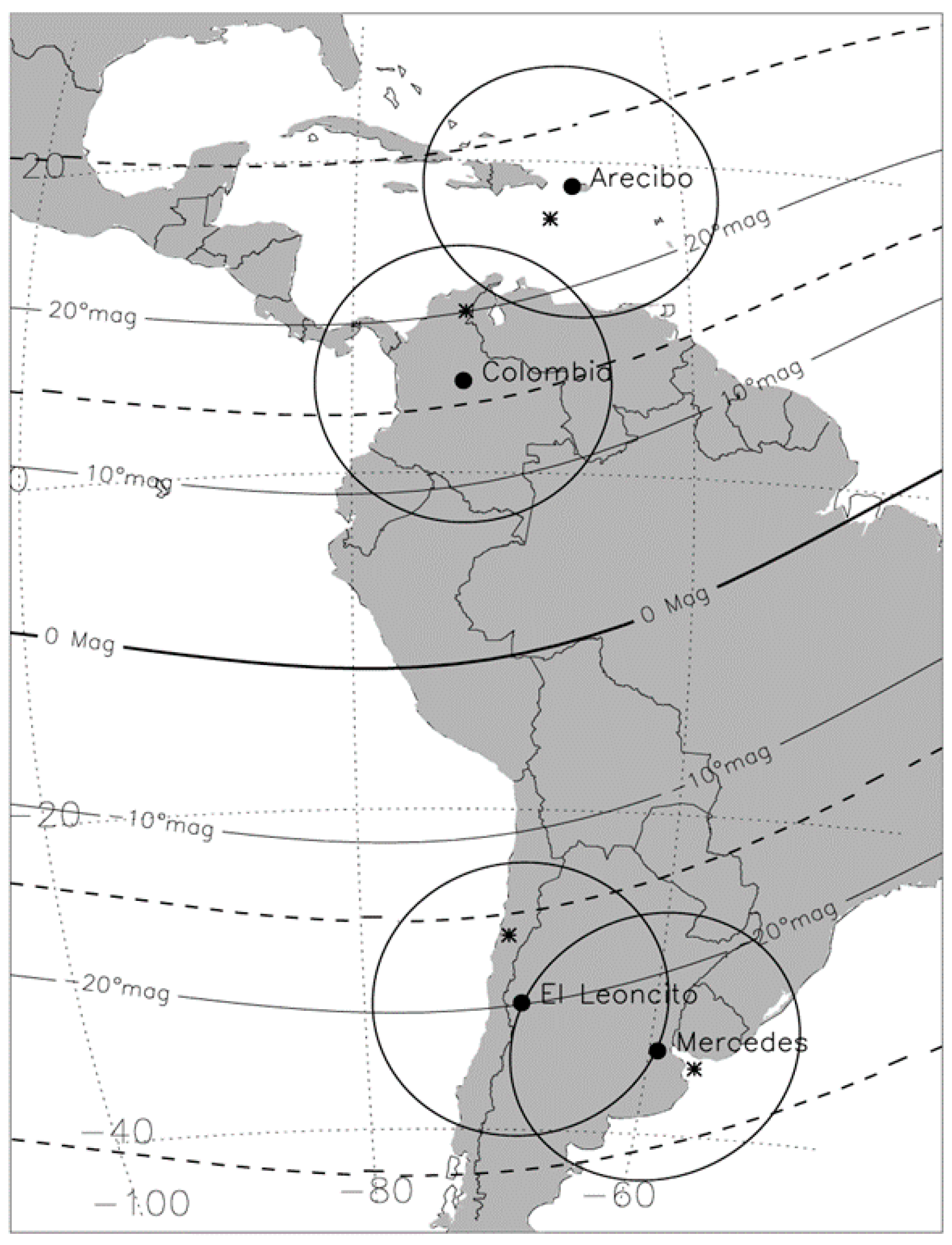
2. Observations
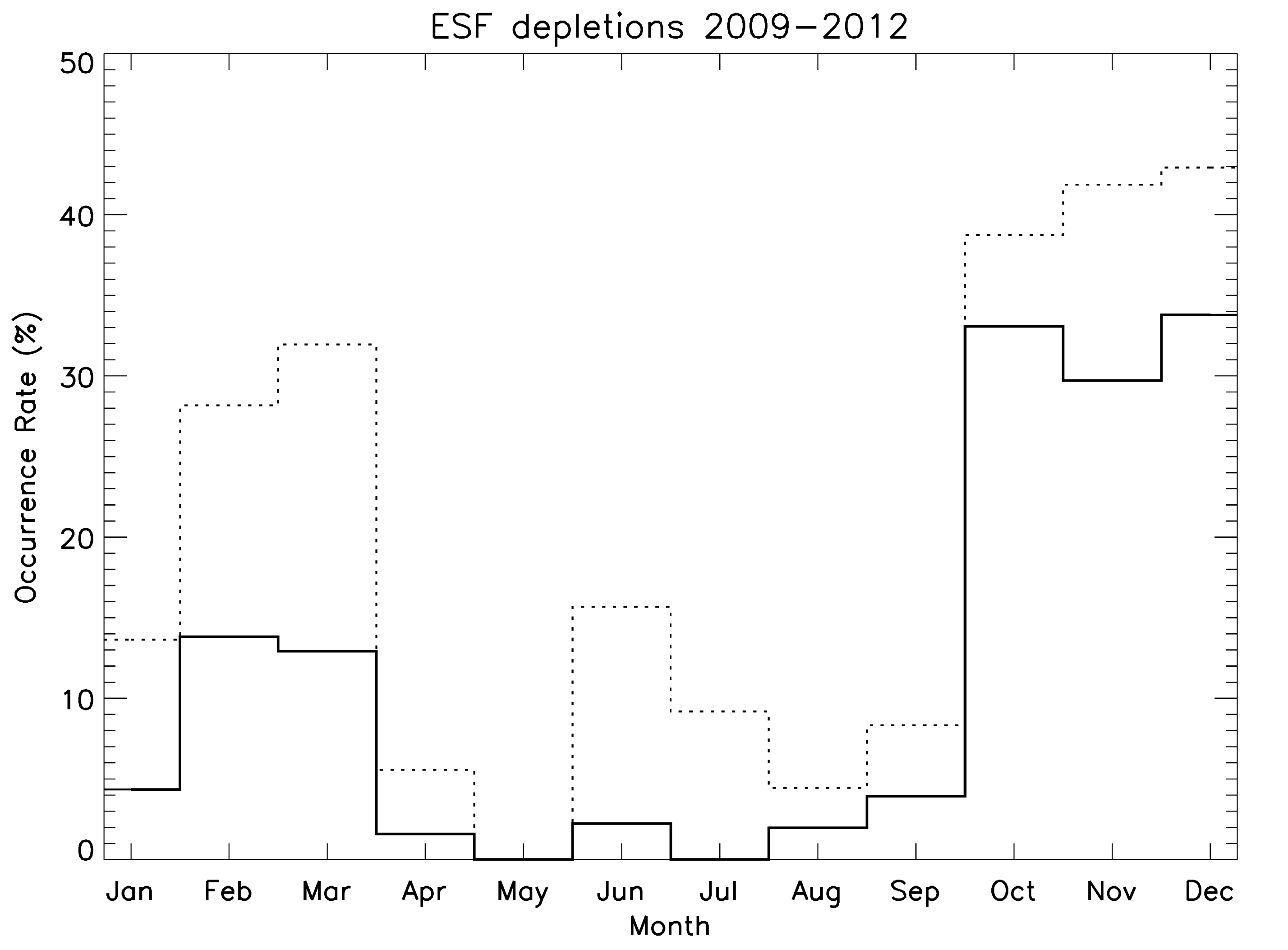
2.1. Arecibo ESF Depletions
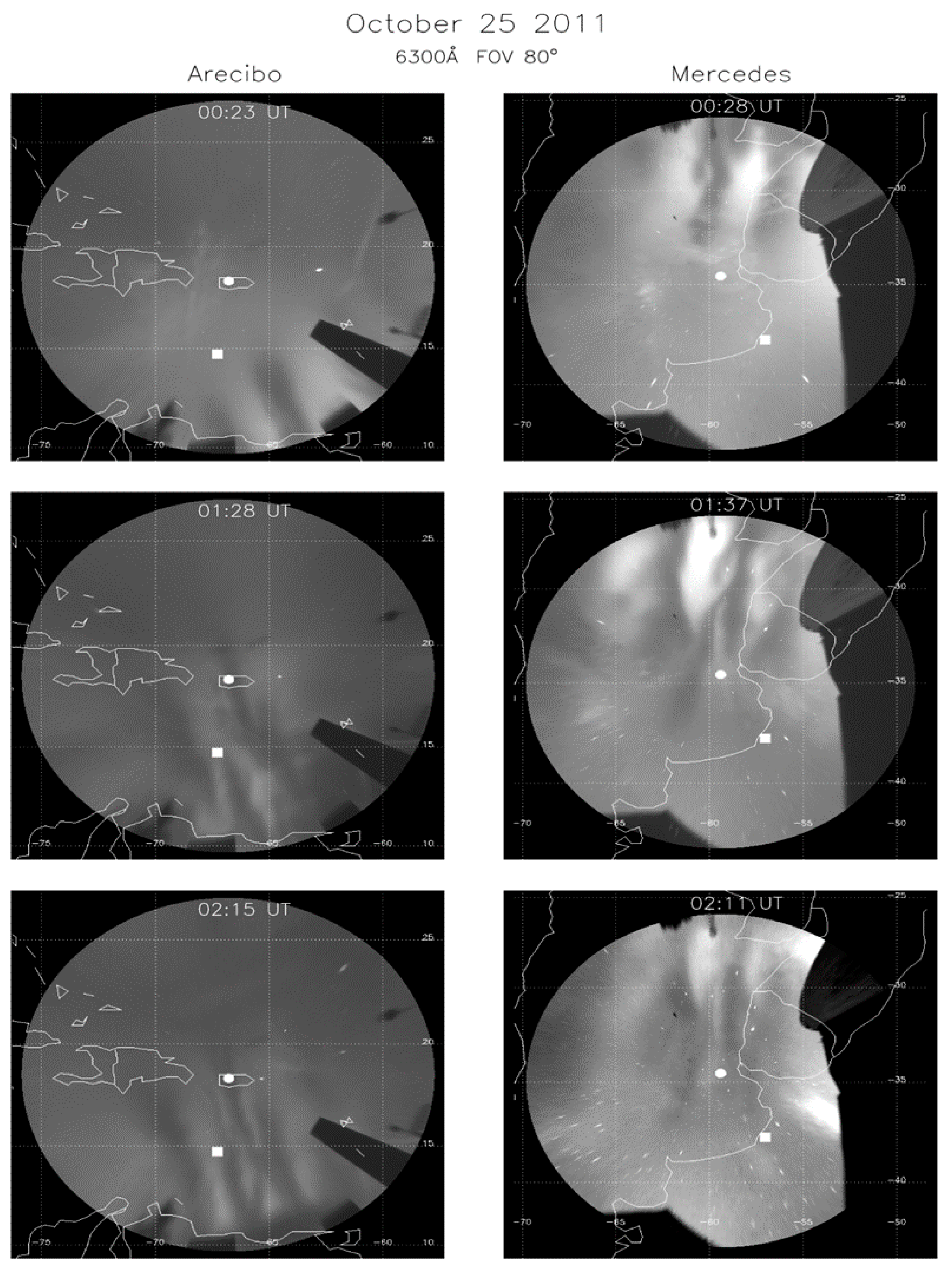
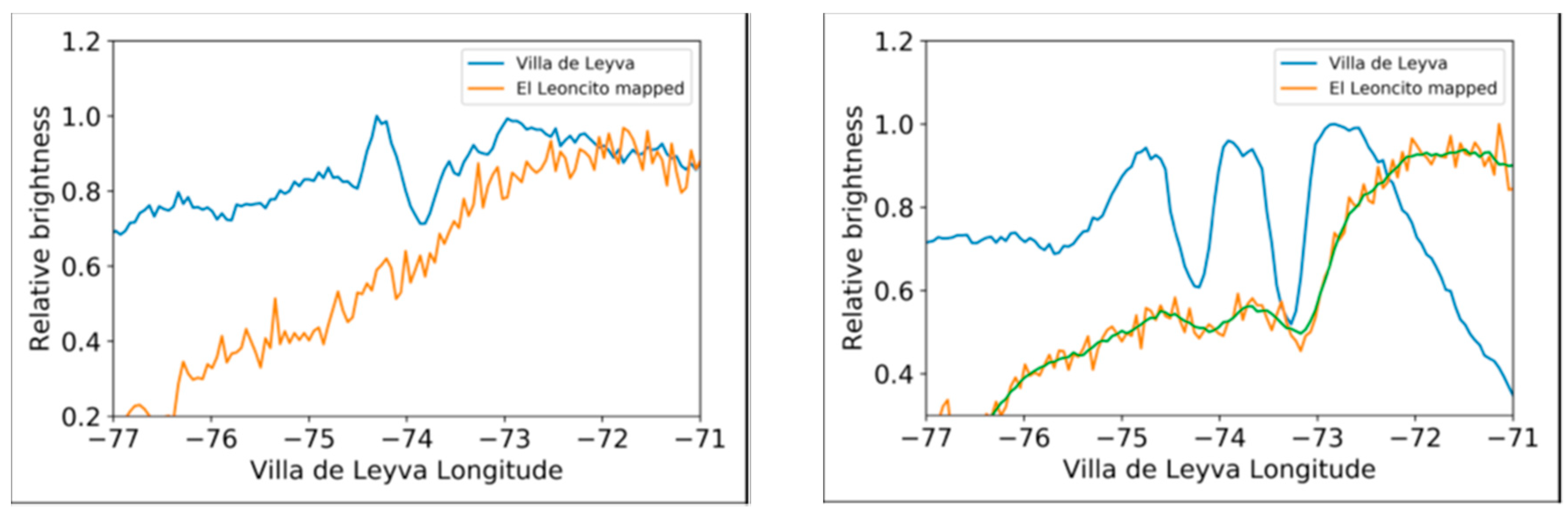
2.2. Magnetically Conjugate Observations
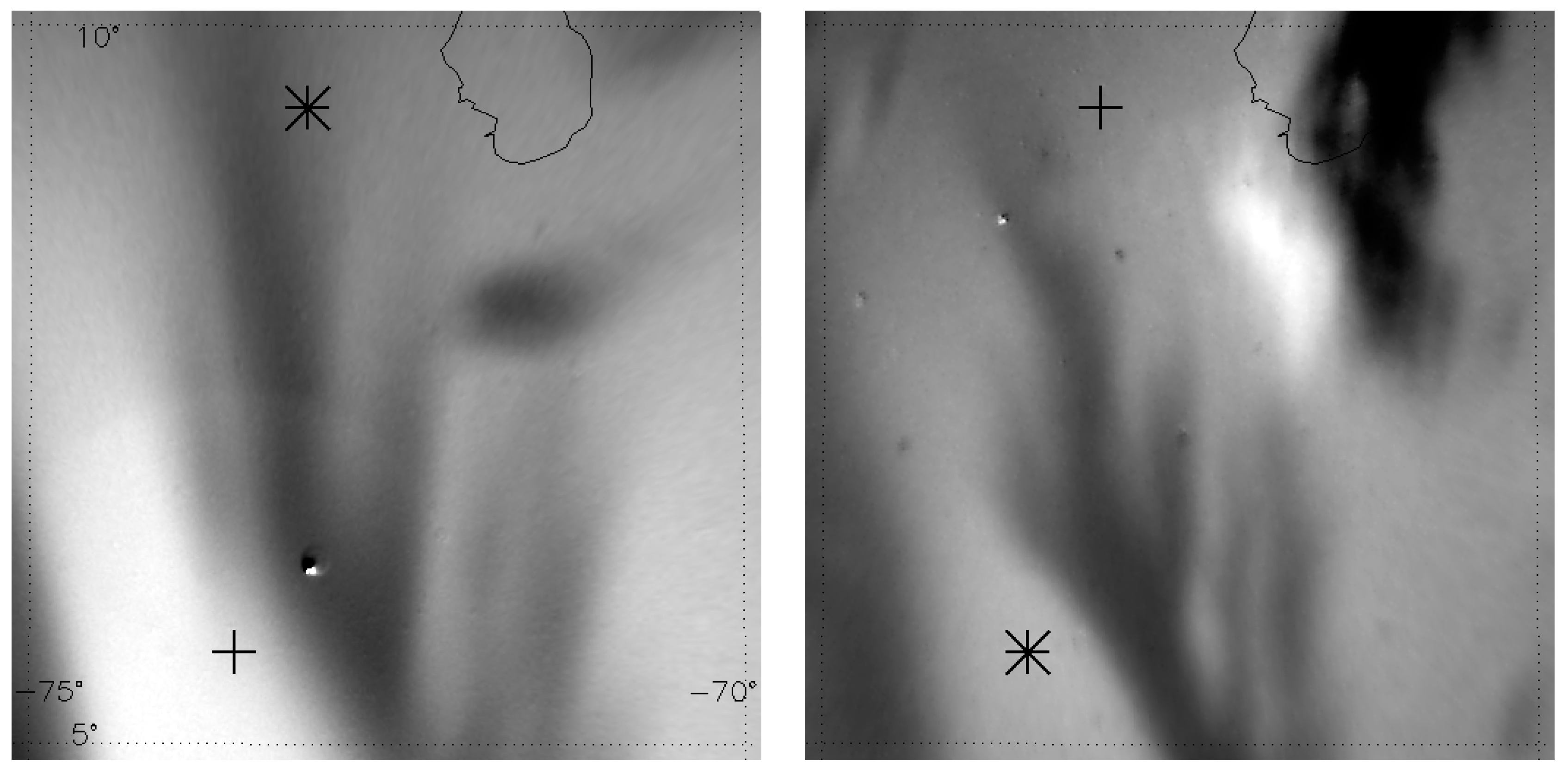
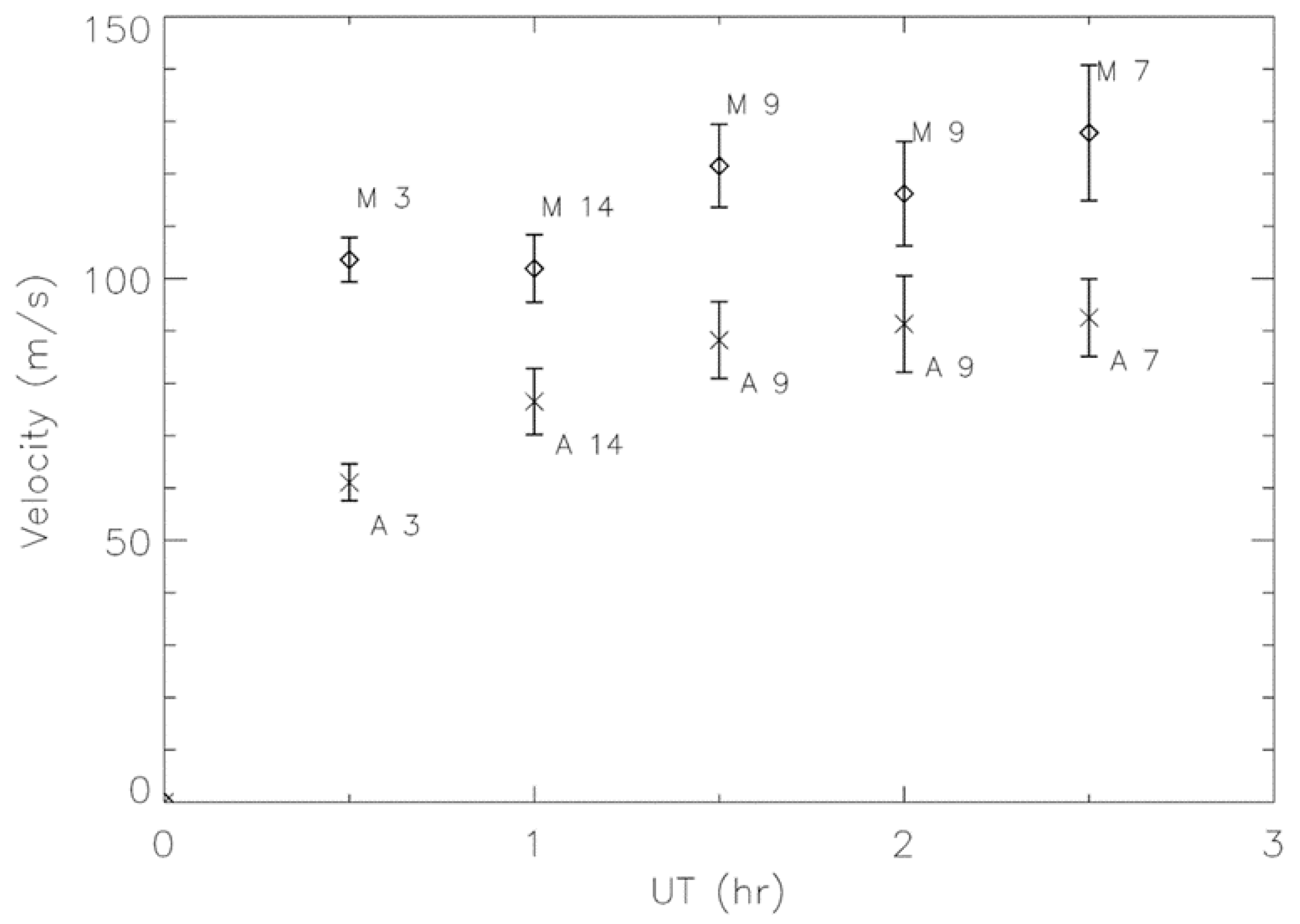
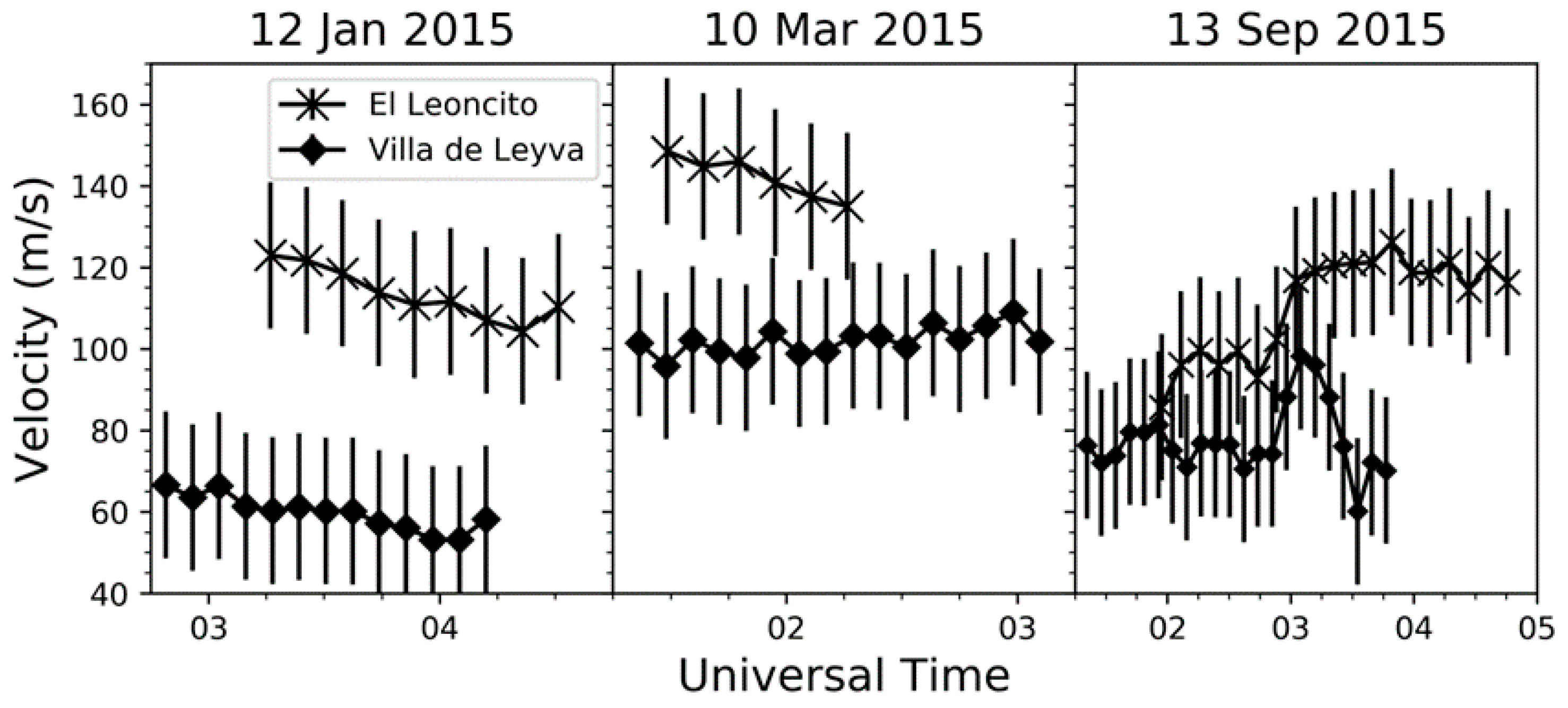
2.3. Magnetically Conjugate Zonal Velocities
3. Discussion
4. Conclusions
Author Contributions
Funding
Acknowledgments
Conflicts of Interest
References
- Martinis, C.; Baumgardner, J.; Wroten, J.; Mendillo, M. All-sky-imaging capabilities for ionospheric space weather research using geomagnetic conjugate point observing sites. Adv. Space Res. 2018, 61, 1636–1651. [Google Scholar] [CrossRef]
- Hickey, D.A.; Sau, S.; Narayanan, V.L.; Gurubaran, S. A possible explanation of interhemispheric asymmetry of equatorial plasma bubbles in airglow images. J. Geophys. Res. Space 2020, 125, e2019JA027592. [Google Scholar] [CrossRef]
- Bilitza, D.; Altadill, D.; Truhlik, V.; Shubin, V.; Galkin, I.; Reinisch, B.; Huang, X. International reference ionosphere 2016: From ionospheric climate to real-time weather predictions. Space Weather 2017, 15, 418–429. [Google Scholar] [CrossRef]
- Picone, J.M.; Hedin, A.E.; Drob, D.P.; Aikin, A.C. NRLMSISE-00 empirical model of the atmosphere: Statistical comparisons and scientific issues. J. Geophys. Res. 2002, 107, 1468. [Google Scholar] [CrossRef]
- Martinis, C.; Mendillo, M. Equatorial spread F-related airglow depletions at Arecibo and conjugate observations. J. Geophys. Res. 2007, 112, A10310. [Google Scholar] [CrossRef]
- Martinis, C.; Baumgardner, J.; Wroten, J.; Mendillo, M. Seasonal dependence of MSTIDs obtained from 630.0 nm airglow imaging at Arecibo. Geophys. Res. Lett. 2010, 37, L11103. [Google Scholar] [CrossRef]
- Shiokawa, K.; Ihara, C.; Otsuka, Y.; Ogawa, T. Statistical study of nighttime medium-scale traveling ionospheric disturbances using midlatitude airglow images. J. Geophys. Res. 2003, 108, 1052. [Google Scholar] [CrossRef]
- Martinis, C.; Baumgardner, J.; Wroten, J.; Mendillo, M. All-sky imaging observations of conjugate medium-scale traveling ionospheric disturbances in the American sector. J. Geophys. Res. 2011, 116, A05326. [Google Scholar] [CrossRef]
- Aarons, J. The longitudinal morphology of equatorial F-layer irregularities relevant to their occurrence. Space Sci. Rev. 1993, 63, 209–243. [Google Scholar] [CrossRef]
- Burke, W.; Huang, C.; Gentile, L.; Bauer, L. Seasonal-longitudinal variability of equatorial plasma bubbles. Ann. Gepphys. 2004, 22, 3089–3098. [Google Scholar] [CrossRef]
- Aa, E.; Zou, S.; Liu, S. Statistical analysis of equatorial plasma irregularities retrieved from Swarm 2013–2019 observations. J. Geophys. Res. Space 2020, 125, e2019JA027022. [Google Scholar] [CrossRef]
- Martinis, C.; Mendillo, M.; Aarons, J. Toward a synthesis of equatorial spread-F (ESF) onset and suppression during geomagnetic storms. J. Geophys. Res. 2005, 110, A07306. [Google Scholar] [CrossRef]
- Hickey, D.A.; Martinis, C.R.; Mendillo, M.; Baumgardner, J.; Wroten, J.; Milla, M. Simultaneous 6300 Å airglow and radar observations of ionospheric irregularities and dynamics at the geomagnetic equator. Ann. Geophys. 2018, 36, 473–487. [Google Scholar] [CrossRef]
- Martinis, C.; Eccles, J.V.; Baumgardner, J.; Manzano, J.; Mendillo, M. Latitude dependence of zonal plasma drifts obtained from dual-site airglow observations. J. Geophys. Res. 2003, 108, 1129. [Google Scholar] [CrossRef]
- Sobral, J.H.A.; Abdu, M.A.; Pedersen, T.R.; Castilho, V.; Arruda, D.; Muella, M.; Batista, I.; Mascarenhas, M.; de Paula, E.; Kintner, P. Ionospheric zonal velocities at conjugate points over Brazil during the COPEX campaign: Experimental observations and theoretical validations. J. Geophys. Res. 2009, 114, A04309. [Google Scholar] [CrossRef]
- Chapagain, N.P.; Fisher, D.J.; Meriwether, J.W. Comparison of zonal neutral winds with equatorial plasma bubble and plasma drift velocities. J. Geophys. Res. Space Phys. 2013, 118, 1802–1812. [Google Scholar] [CrossRef]
- Fukushima, D.; Shiokawa, K.; Otsuka, Y.; Nishioka, M.; Kubota, M.; Tsugawa, T.; Nagatsuma, T.; Komonjinda, S.; Yatini, C.Y. Geomagnetically conjugate observation of plasma bubbles and thermospheric neutral winds at low latitudes. J. Geophys. Res. Space Phys. 2015, 120, 2222–2231. [Google Scholar] [CrossRef]
- Kelley, M.C.; Makela, J.J.; Paxton, L.J.; Kamalabadi, F.; Comberiate, J.M.; Kil, H. The first coordinated ground- and space-based optical observations of equatorial plasma bubbles. Geophys. Res. Lett. 2003, 30, 1766. [Google Scholar] [CrossRef]
- Otsuka, Y.; Shiokawa, K.; Ogawa, T.; Wilkinson, P. Geomagnetic conjugate observations of equatorial airglow depletions. Geophys. Res. Lett. 2002, 29, 15. [Google Scholar] [CrossRef]
- Abdu, M.A.; Batista, I.S.; Reinisch, B.W.; de Souza, J.R.; Sobral, J.H.A.; Pedersen, T.R.; Medeiros, A.F.; Schuch, N.J.; de Paula, E.R.; Groves, K.M. Conjugate Point Equatorial Experiment (COPEX) campaign in Brazil: Electrodynamics highlights on spread F development conditions and day-to-day variability. J. Geophys. Res. 2009, 114, A04308. [Google Scholar] [CrossRef]
- Ma, G.; Maruyama, T. A super bubble detected by dense GPS network at east Asian longitudes. Geophys. Res. Lett. 2006, 33, L21103. [Google Scholar] [CrossRef]
- Martinis, C.; Baumgardner, J.; Mendillo, M.; Wroten, J.; Coster, A.; Paxton, L. The night when the auroral and equatorial ionospheres converged. J. Geophys. Res. Space Phys. 2015, 120, 8085–8095. [Google Scholar] [CrossRef]
- Aa, E.; Zou, S.; Ridley, A.J.; Zhang, S.; Coster, A.; Erickson, P.; Liu, S.; Ren, J. Merging of storm time midlatitude traveling ionospheric disturbances and equatorial plasma bubbles. Space Weather 2019, 17, 285–298. [Google Scholar] [CrossRef]
- Mendillo, M.; Zesta, E.; Shodhan, S.; Sultan, P. Observations and modeling of the coupled latitude-altitude patterns of equatorial plasma depletions. J. Geophys. Res. 2005, 110, A09303. [Google Scholar] [CrossRef]
- Krall, J.; Huba, J.D.; Martinis, C. Three-dimensional modeling of equatorial spread-F airglow enhancements. Geophys. Res. Lett. 2009, 36, L10103. [Google Scholar] [CrossRef]
- Krall, J.; Huba, J.D.; Ossakow, S.L.; Joyce, G. Why do equatorial ionospheric bubbles stop rising? Geophys. Res. Lett. 2010, 37, L09105. [Google Scholar] [CrossRef]
- Thébault, E.; Finlay, C.C.; Beggan, C.D.; Alken, P.; Aubert, J.; Barrois, O.; Bertrand, F.; Bondar, T.; Boness, A.; Brocco, L. International Geomagnetic Reference Field: The 12th generation. Earth Planets Space 2015, 67, 79. [Google Scholar] [CrossRef]
- Rishbeth, H. Thermospheric winds and the F-region: A review. J. Atmos. Terr. Phys. 1972, 34, 1–47. [Google Scholar] [CrossRef]
- Drob, D.P.; Emmert, J.T.; Meriwether, J.W.; Makela, J.; Doornbos, J.; Conde, M.; Hernandez, G.; Noto, J.; Zawdie, K.A.; McDonald, S.E. An update to the Horizontal Wind Model (HWM): The quiet time thermosphere. Earth Space Sci. 2015, 2, 301–319. [Google Scholar] [CrossRef]
- Laundal, K.M.; Richmond, A.D. Magnetic Coordinate Systems. Space Sci. Rev. 2017, 206, 27–59. [Google Scholar] [CrossRef]


| Year | <F10.7> | # Cases Arecibo | # Cases Mercedes | # Simultaneous |
|---|---|---|---|---|
| 2009 | 69 | 5 | 15 | 3 |
| 2010 | 80 | 13 | 33 | 7 |
| 2011 | 113 | 45 | 67 | 27 |
| January–February 2012 | 113 | 18 | 17 | 14 |
| Total | 81 | 122 | 51 |
© 2020 by the authors. Licensee MDPI, Basel, Switzerland. This article is an open access article distributed under the terms and conditions of the Creative Commons Attribution (CC BY) license (http://creativecommons.org/licenses/by/4.0/).
Share and Cite
Martinis, C.; Hickey, D.; Wroten, J.; Baumgardner, J.; Macinnis, R.; Sullivan, C.; Padilla, S. All-Sky Imager Observations of the Latitudinal Extent and Zonal Motion of Magnetically Conjugate 630.0 nm Airglow Depletions. Atmosphere 2020, 11, 642. https://doi.org/10.3390/atmos11060642
Martinis C, Hickey D, Wroten J, Baumgardner J, Macinnis R, Sullivan C, Padilla S. All-Sky Imager Observations of the Latitudinal Extent and Zonal Motion of Magnetically Conjugate 630.0 nm Airglow Depletions. Atmosphere. 2020; 11(6):642. https://doi.org/10.3390/atmos11060642
Chicago/Turabian StyleMartinis, Carlos, Dustin Hickey, Joei Wroten, Jeffrey Baumgardner, Rebecca Macinnis, Caity Sullivan, and Santiago Padilla. 2020. "All-Sky Imager Observations of the Latitudinal Extent and Zonal Motion of Magnetically Conjugate 630.0 nm Airglow Depletions" Atmosphere 11, no. 6: 642. https://doi.org/10.3390/atmos11060642
APA StyleMartinis, C., Hickey, D., Wroten, J., Baumgardner, J., Macinnis, R., Sullivan, C., & Padilla, S. (2020). All-Sky Imager Observations of the Latitudinal Extent and Zonal Motion of Magnetically Conjugate 630.0 nm Airglow Depletions. Atmosphere, 11(6), 642. https://doi.org/10.3390/atmos11060642