Abstract
Seasonal Auto Regressive Integrative Moving Average models (SARIMA) were developed for monthly rainfall time series. Normality of the rainfall time series was achieved by using the Box Cox transformation. The best SARIMA models were selected based on their autocorrelation function (ACF), partial autocorrelation function (PACF), and the minimum values of the Akaike Information Criterion (AIC). The result of the Ljung–Box statistical test shows the randomness and homogeneity of each model residuals. The performance and validation of the SARIMA models were evaluated based on various statistical measures, among these, the Student’s t-test. It is possible to obtain synthetic records that preserve the statistical characteristics of the historical record through the SARIMA models. Finally, the results obtained can be applied to various hydrological and water resources management studies. This will certainly assist policy and decision-makers to establish strategies, priorities, and the proper use of water resources in the Sinú river watershed.
1. Introduction
Precipitation is one of the variables commonly used to study climate variability. It is the result of the interaction of various physical phenomena and is characterized by its spatial and temporal variation. Thus, the analysis of rainfall data is essential for the prediction of meteorological information and also for the planning and management of water resource systems [1,2,3,4].
Missing data are a very frequent problem in climatology, and they influence the quality of the results, impacting hydrological studies as well as water resource management. These studies require complete and reliable records of rainfall data. Some methods to solve the problem of the reliability of obtained results and findings can be found in the literature [5,6,7,8]. Among these, stochastic models stand out. They are used to generate synthetic time series, which exhibit similar statistical characteristics to the observed data and behave according to probabilistic laws. Consequently, the observed series is only one of the possible achievements of the stochastic process and, thus, the forecast is not an exact but a possible scenario [9]. For instance, Autoregressive Moving Average (ARMA) models are stochastic models based on probability theory, so they can represent the temporal uncertainty of data. They originate from the research of Yule [10,11], who first described Autoregressive (AR) models; Slutzky [12], who proposed Moving Average (MA) models; and Wold [13], who introduced ARMA mixed models.
In addition, there are variations of autoregressive models, such as Periodic Autorregressive Moving Average (PARMA) models; ARMA models with the Auxiliary inputs, ARMAX; Autoregressive Interated Moving Average (ARIMA) models; and ARIMA models with seasonal components or Seasonal Auto Regressive Integrative Moving Average (SARIMA), which allow the user to generate synthetic time series considering cyclical variations in the observed series records [9,14].
Among the applications of stochastic models for forecasting rainfall, it is important to mention works such as the one from Sanvicente-Sanchez and Solis-Alvarado [15], who proposed a method to generate a synthetic series of daily precipitation, seeking to preserve the spatial, temporal, and magnitude correlation of rain in a network of weather stations or in a watershed divided into sub-watersheds. On the other hand, Lee [16] combined the Markov chains (AR models describing a sequence of possible events in which the probability of each event depends only on the state achieved in the previous event) with ARMA models to generate a synthetic time series [17,18]. By using SARIMA models to analyze the daily and hourly rainfall data, Bang et al. [19] compared the performance of ARMA, SARIMA, and ARMAX models to predict rainfall and temperature in India, finding that temperature is best predicted by the SARIMA model and that the accuracy of predictions made for rainfall by the ARMA model is better than those made by the ARMAX model.
Another area of potential breakthrough is the possible enhancement of forecasts for weather and climate phenomena, such as El Niño–Southern Oscillation (ENSO) in the tropical Pacific and La Niña (adverse cold effects). Such events are related to a variation of ±0.5 °C in the sea surface temperature averaged over three consecutive months [20]. Sun and Furbish [21] found high values of correlation coefficients between the sea surface temperature data and a precipitation series, studied using ARMA (0,1) models. They showed that the El Niño and La Niña events are responsible for 40% of annual precipitation variations and up to 30% of river discharge variations in Florida. In this context, some studies use Smooth Transition Autoregressive (STAR) for nonlinear time series modeling. The results revealed STAR-type nonlinearities in ENSO dynamics, resulting in the superior sample forecast performance of STAR over the linear autoregressive models [22]. Likewise, Arganis et al. [23] proposed a procedure to determine sea surface temperatures through the combination of the Fiering and Svanidze methods, overcoming deficiencies that appeared in the Svanidze and ARMA–Svanidze models and allowing the analysis of the possible long term behavior of the values for sea surface temperature and the modelling of “El Niño” or “La Niña” episodes in Mexico.
Despite the fact that nonlinear models such as Artificial Neural Networks, Artificial Intelligence models, Genetic Programming, and Chaos Theory techniques have been successfully used as suitable tools for modeling and forecasting meteorological information such as precipitation and runoff [24,25,26,27,28], the versatility of stochastic models has been proved. Consequently, a wide range of improvements to the procedures traditionally used can be found [29,30,31,32,33,34,35,36,37,38].
In general, stochastic models have made possible the study of several autocorrelation functions of the hydro–climatological variables used to describe the processes of the hydrologic cycle. Furthermore, hydrological time series modeling based on stochastic models has been confirmed by many researchers, because these models are a proper choice for areas where nothing but the hydrological time series data is available [1]. Thus, stochastic models are still suitable for analyzing and forecasting the variables of the hydrological cycle, such as precipitation, in a reliable way [39,40,41,42].
Finally, data generation is an important subject in stochastic hydrology and is used by hydrologists for many purposes. These include, for example, reservoir sizing and planning, water resources management, and climate variability analyses.
This article proposes the SARIMA approach to generating synthetic monthly rainfall in the Sinú river watershed in Colombia. The aspects considered are the model form identification, parameter estimation techniques, seasonal time series modeling, and the effects of different model time increments.
2. Materials and Methods
2.1. Study Area
The Sinú River watershed is in Northwestern Colombia between 9°30’ N and 7°05’ N and 76°35’ W and 75°15’ W (Figure 1), with an area of 13,972 km2 and in the jurisdiction of the Córdoba, Sucre, and Antioquia departments. According to the Autonomous Regional Corporation of the Valleys of Sinú and San Jorge (CVS), the watershed is divided according to its physical and biotic characteristics into 3 zones: Upper, Middle, and Lower Sinú [43]. It should be noted that the main populated communities in the watershed are Tierralta and Valencia in the upper watershed, Montería (capital of the Córdoba department) in the middle one, and Lorica in the lower one. Additionally, the URRÁ hydroelectric power plant and the Paramillo National Natural Park are located in the upper watershed [44].
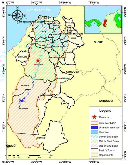
Figure 1.
Sinú river watershed location in Colombia. Montería city is observed to be the most representative urban area, along with the Sinú river and the URRÁ hydroelectric power plant.
Furthermore, according to information extracted from the climatological stations by the Colombian Institute of Hydrology, Meteorology, and Environmental Studies (IDEAM), the Sinú river watershed is known for having a unimodal rainfall regime, with a dry season and rainy season per year. The rainy season begins in April and ends in November, during which more than 80% of the annual rainfall occurs. Extreme rainfall events appear in the Upper Sinú basin, reaching magnitudes of greater than 4000 mm annually and decreasing from south to north. Thus, in the lower part of the river (delta) the precipitation is about 1300 mm. Similarly, it was evident that the average air temperature is above 27 °C and varies from south to north as the precipitation does. Consequently, in the upper Sinú there are temperatures of up to 17 °C, while in the rest of the basin the temperature exceeds 32 °C.
The data used for the modeling were obtained from 75 climatological stations (Figure 2) from the IDEAM database, and it was verifyied that they had influence in the study area using Thiessen Polygons [45]. The missing rainfall data were estimated using the ClimGen model [46,47]. To gain information to validate the models obtained, the original data were divided so that a calibration vector was obtained that corresponded to the first 90% of the data and a validation vector was obtained that was equivalent to the remaining 10%. This criterion was chosen considering what was reported by Dabral and Murry [48] and Nury et al. [49]. This allows the user to make a forecast with the selected model and compare the observed and predicted rainfall during the period corresponding to the validation vector.
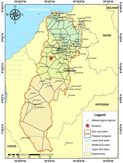
Figure 2.
Spatial locations of the selected rainfall stations and Thiessen polygons for the 75 selected stations in the Sinú river watershed (Colombia).
To guarantee the normality of the calibration vectors, a transformation was performed to make the transformed data approximately Gaussian and stabilize the variance of the time series. Although there are many families of transformations which may be used for such a purpose, the Box–Cox power transformation was found to be useful in various fields including hydrology and meteorology, as reported by Chatfield [50] and Dabral and Murry [48]. Given an observed time series, xt, the transformed series is given by:
where yt is the Box–Cox transformed data and λ denotes the power parameter chosen to make the transformed data approximately Gaussian.
Before determining the optimal forecast model, a filtering procedure was performed. The transformed calibration vectors were decomposed in three components: trend, seasonal, and remainder. According to Cleveland et al. [51], the trend component is the low frequency variation in the data together with nonstationary, long-term changes in the level; the seasonal component is the variation in the data at or near the seasonal frequency, normally one cycle per year; and the remainder component is the remaining variation in the data beyond that in the seasonal and trend components [1,52]. The equation of the additive decomposition is:
where the time series, trend component, seasonal component, and the remainder component are denoted by Xt, Tt, St, and Rt, respectively.
2.2. SARIMA Models
The SARIMA model is based on the application of the ARMA models to a transformed time series where the seasonal and non-stationary behavior has been eliminated.
For a seasonal series with s periods per year, the SARIMA(p,d,q) × (P,D,Q)s models are used. Thus, having a Bs operator such that BsXt = Xt−s and since the seasonal difference can be written as (Xt − Xt−s) = (1 − Bs)Xt, a SARIMA model with (p,d,q) non-seasonal order terms and (P,D,Q) seasonal order terms—SARIMA(p,d,q) × (P,D,Q)s—has the following structure [50]:
where Φ(Bs) and Θ(Bs) denote polynomials in Bs with P and Q order, respectively, while ϕ(B) and θ(B) are polynomials in B with p and q order, respectively.
Four stages were followed to determine the optimal forecast model in each station: identification, estimation, verification, and application or forecast, as suggested by Box et al. [53], Salas and Obeysekera [54], and Burlando et al. [55]. In the first instance, it was required to verify the data stationarity, and the general form or model order was estimated. Then, the model parameters were estimated using the maximum likelihood method, and the model suitability was verified using the Ljung–Box statistical test to prove that the residuals behaved as white noise [56]. The optimal model was chosen from among those that satisfactorily adjusted the data. There are several tools, such as the Bayesian Information Criterion (BIC), Hannan–Quinn criterion (H–Q), and the coefficient of determination (R2), to determine the best model [1,49]. However, in most of the carried-out research, the Autocorrelation Function (ACF) and the Partial Autocorrelation Function (PACF) have been used to select the optimal model. Considering this, the ACF and PACF were used to determine the best type of model. The Akaike Information Criterion (AIC) of each model was estimated and the one with the lowest AIC was chosen [53,57].
Finally, once the optimal model was determined, the forecast was made and the results were compared with the validation vector to evaluate the performance. For all this, an algorithm was designed in the programming language for statistical analysis “R”, which also allowed us to identify the most suitable forecast model from the AIC. Thus, different model options, such as AR, MA, ARMA, ARIMA, and SARIMA, were tested, and it was determined that the models that showed the best performance were the SARIMA.
3. Results and Discussion
To illustrate the methodology used to determine the optimal forecast models, the results from the Momil station will be used as an example. The corresponding calibration vector can be observed in Figure 3. First, to guarantee the normality of the series, a data transformation was performed using Box–Cox (Figure 4); then, the Augmented Dickey–Fuller test (ADF), a unit root test that allows accepting or rejecting the null hypothesis of stationarity in a time series for validation, was used [48,58].
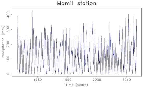
Figure 3.
Calibration vector of the monthly precipitation time series.
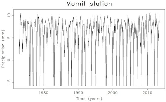
Figure 4.
Calibration vector of the transformed monthly precipitation time series using Box–Cox.
In the Momil station transformed series graph (Figure 4), peaks are observed approximately once a year, which may be indicators that the series exhibits seasonal behavior. Nonetheless, although it is not graphically possible to confirm the seasonality presence, it is possible by decomposing the time series since it allows determining the series components (trend, seasonality, random components) and analyzing their structure. In this way, Figure 5 shows the additive decomposition of the series in question, where it is possible to identify that the series has a marked seasonality that mainly obeys the unimodal precipitation regime typical from the area; it is evident that a trend is not maintained throughout the series period.
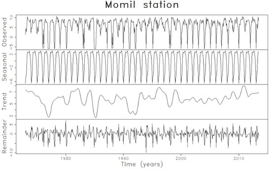
Figure 5.
Decomposition of the calibration vector of the transformed precipitation time series using Box–Cox (time series graphs with random, seasonal, and trend components).
Bearing this in mind, it is inferred that s = 12, i.e., the number of periods per year is 12 (one period per month). To check the latter, the series correlograms were calculated from the ACF and the PACF, as shown in Figure 6 and Figure 7, where indeed it was possible to see that the highest correlation occurs when the lag k is 12, indicating that values of a specific month have a greater relationship with those shown in the same month from the immediately previous year.
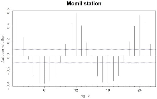
Figure 6.
Autocorrelation function (ACF) of the calibration vector of the transformed precipitation time series using Box–Cox.
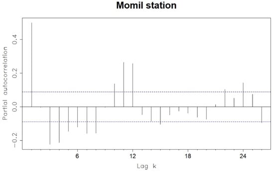
Figure 7.
Partial autocorrelation function (PACF) of the calibration vector of the transformed precipitation time series using Box–Cox.
Moreover, the correlograms (Figure 6 and Figure 7) show a sinusoidal shape, which additionally suggests that the SARIMA model is the most appropriate one to represent the precipitation series of the Momil station. Thus, the different models were adjusted until the optimal one was selected using the AIC. The best fit model was SARIMA (2,0,0) × (2,1,0)12, which was selected based on the minimum values of AIC = 2433.6 (Table 1). The simplified general equation is:
where the parameters ϕp and Φp are observed on the left, multiplying the values of Xt times the different lags, i.e., values that the variable took before the instant of interest time. In this case, since there are two parameters ϕp, it implies that the two previous values of Xt, will be multiplied, i.e., it goes back two months in the non-seasonal component, or the same as the model will use the precipitation values of the two immediately preceding months to calculate rainfall at a given point in time. On the other hand, the two parameters Φp of the seasonal component imply that the model considers the values of the previous 2 years for the month analyzed. Thus, the equation of the SARIMA (2,0,0) × (2,1,0)12 is the resulting one from solving the product of the polynomials shown in the simplified general equation until arriving at the following expression:

Table 1.
Akaike Information Criterion (AIC) from some of the forecast models tested at the Momil station.
Figure 8 shows the synthetic series generated (predicted data). It shows that the model can represent both the magnitude of the recorded rainfall and its variation.
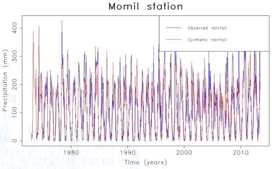
Figure 8.
Observed precipitation (calibration vector) and synthetic time series.
Then, the residuals were analyzed using the Ljung–Box test and correlograms (Figure 9). The correlograms show significant peaks in lags 24 and 25, indicating that those order models could more represent the series structure. Nonetheless, using the AIC based on the parsimony principle that the greater the number of parameters of a model, the greater its complexity, and a solution must be sought that allows maintaining a balance between the adjustment and complexity, it is concluded that the best model is the one selected, since it has minimum values of Akaike information criterion (AIC) and therefore uses the fewest parameters to generate a synthetic series. The result of the Ljung–Box statistic test shows the randomness and homogeneity of the residuals. Thus, the SARIMA model is appropriate for forecasting. At this point, it is important to highlight that, although the residuals’ analysis is considered important for the analysis of the model’s performance, there could be a case where the Ljung–Box test indicates that they are not random for a given significance level. Even so, if the model can adequately represent the series’ behavior and preserve the mean of the original data, it is concluded that the selected model is the most appropriate among all those tested and can be used to make forecasts (Figure 10).
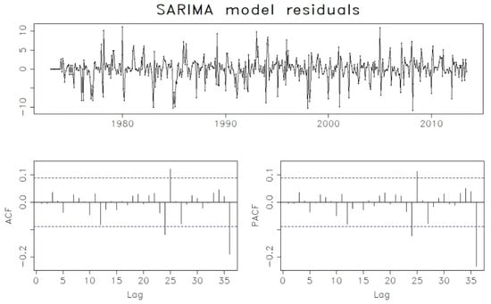
Figure 9.
Residuals from the Seasonal Auto Regressive Integrative Moving Average (SARIMA) model.
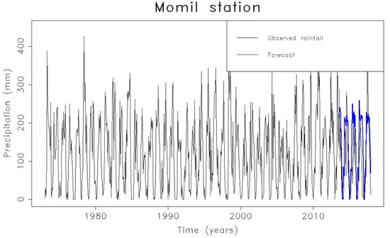
Figure 10.
Model prediction versus the observed values.
Subsequently, a test of hypothesis concerning the difference between two means with student’s t-distribution was used to compare the mean of the calibration vector with that of the synthetic series, and in the same way compare the validation vector mean with that of the forecast obtained [59]. The null hypothesis is that the difference in the means of the two datasets is equal to 0, therefore the alternative hypothesis is that difference in means is not equal to 0.
In the Momil station case, Table 2 shows that at a 5% significance level there is no statistically significant difference between the means of the calibration vector and the synthetic series. This is because the p value (0.15) is greater than 0.05 and because the 95% confidence interval (−3.15, 20.4) includes the 0 value. The above implies that by using the SARIMA model (2,0,0) × (2,1,0)12, a synthetic series statistically equal to the original can be obtained, and therefore it is the optimal model for the Momil station.
Table 2.
Hypothesis test regarding the difference between the two means from the Momil station.
Finally, when comparing the means of the validation vector and the forecast, it was concluded that at a 2% significance level there is no statistically significant difference, since the p-value (0.023) is greater than 0.02 and the 98% confidence interval (−0.82, 79.65) includes the 0 value (Table 2). The test was performed for a confidence level of 98% for the comparison between the validation vector and the forecast since, in this way, there was a greater probability that the hypothesis was satisfied.
Since the validation series and the forecast are determined to be statistically the same, it is considered that the SARIMA (2,0,0) × (2,1,0)12 model adequately represents the data structure from the Momil station and is appropriate for forecasting precipitation. Table 3 shows the optimal model for all the climatological stations in the study area.
Table 3.
SARIMA models for modeling and forecasting the monthly rainfall in the Sinú river watershed in Colombia.
4. Conclusions
This study focused on modeling and forecasting a monthly rainfall series using SARIMA modeling. The results obtained can be applied for various hydrological and water resource management studies. This will certainly assist policy and decision-makers to establish strategies, priorities, and the proper use of water resources in the Sinú river watershed—e.g., the proposed models can be used to determine the occurrence of the El Niño-–Southern Oscillation phenomena, to identify the potential for water harvesting use, and to operate irrigation systems.
The monthly precipitation series recorded in the stations of the study area show a seasonal behavior, reflecting the typical unimodal rain regime from the basin. Similarly, it was determined that a trend was not maintained throughout the recording period.
Through the Box–Cox transformation, it was possible to guarantee the stationarity assumption for the precipitation time series recorded in the Sinú river basin. This allowed us to establish that, given the seasonal behavior of the series analyzed, the SARIMA models allow the satisfactory representation of the temporal structure of precipitation in the study area. The SARIMA approach showed an improvement over the integration of the removal of the trend, periodicity, and stochastic components approach in time series modelling. The different performance statistics in the model development and validation phase of this study also confirmed higher prediction accuracy using the SARIMA models.
By means of the stochastic SARIMA models, it was possible to generate a synthetic time series of precipitation without missing data, which allows us to preserve the behavior and structure of the original data. It was shown that the synthetic series obtained are statistically the same as the observed precipitation, and likewise that the forecasts made using the SARIMA models selected for each season adequately represent the behavior of the rainfall in the area. Based on the results, stochastic models are one of the most appropriate techniques for the prediction of rainfall.
It is important to highlight that although the forecasts obtained with the models do not allow predicting the exact precipitation amount, they can reveal the probable trend of future rains and provide information that can help decision-makers to establish strategies in areas such as agriculture, where it is of utmost importance to know the beginning and end of the rainy seasons the planning of civil works; and the preparation of mitigation plans for natural dangers, such as floods and droughts.
Finally, it is worth noting that rational planning and comprehensive management of water resources require forecasting events that may occur in the future, bearing in mind at the same time that it is usually based on past events. For this reason, time series analysis is a valuable tool since it allows making inferences about the future.
Author Contributions
Conceptualization, discussion and conclusions: Á.A.L.-L., J.P.M.-B., L.M.-A., Á.L.-R. and J.F.R.L.; Material and Methods: J.P.M.-B. and Á.A.L.-L.; Writing—Original Draft Preparation, J.P.M.B. and Á.A.L.-L.; Writing—Review and Editing, Á.A.L.-L.; Visualization, L.M.-A.; Supervision, Á.L.-R., Á.A.L.-L. and J.F.R.L.; Project Administration, Á.A.L.-L., Á.L.-R. and L.M.-A.; Funding Acquisition, J.F.R.L. and L.M.-A. All authors have read and agreed to the published version of the manuscript.
Funding
This research was funded by UNIVERSIDAD PONTIFICIA BOLIVARIANA Seccional Montería, grant number 212-07/17-G018 and HIDRUS S.A de CV. The APC was funded by UNIVERSIDAD PONTIFICIA BOLIVARIANA Seccional Montería.
Acknowledgments
The present study was conducted as a research project number 212-07/17-G018 from the School of Civil Engineering of Universidad Pontificia Bolivariana campus Montería (Colombia), and financed by Universidad Pontificia Bolivariana Seccional Montería, Universidad Autónoma de Baja California campus Ensenada and Hidrus S.A de C.V.
Conflicts of Interest
The authors declare no conflict of interest.
References
- Dastorani, M.; Mirzavand, M.; Dastorani, M.T.; Sadatinejad, S.J. Comparative study among different time series models applied to monthly rainfall forecasting in semi-arid climate condition. Nat. Hazards 2016, 81, 1811–1827. [Google Scholar] [CrossRef]
- Venkata, R.R.; Krishna, B.; Kumar, S.R.; Pandey, N.G. Monthly rainfall prediction using wavelet neural network analysis. Water Resour. Manag. 2013, 27, 3697–3711. [Google Scholar] [CrossRef]
- Li, Y.P.; Nie, S.; Huang, C.Z.; McBean, E.A.; Fan, Y.R.; Huang, G.H. An integrated risk analysis method for planning water resource systems to support sustainable development of an arid region. J. Environ. Inform. 2017, 29, 1–15. [Google Scholar] [CrossRef]
- Radhakrishnan, P.; Dinesh, S. An alternative approach to characterize time series data: Case study on Malaysian rainfall data. Chaos Solitons Fractals 2006, 27, 511–518. [Google Scholar] [CrossRef]
- Wang, S.; Feng, J.; Liu, G. Application of seasonal time series model in the precipitation forecast. Math. Comput. Model. 2013, 58, 677–683. [Google Scholar] [CrossRef]
- Chang, T.J.; Kavvas, M.L.; Delleur, J.W. Daily precipitation modelling by discrete autoregressive moving average processes. Water Resour. Res. 1984, 20, 565–580. [Google Scholar] [CrossRef]
- Ben, A.M.A.; Chebana, F.; Ouarda, T.B.M.J. Probabilistic multisite statistical downscaling for daily precipitation using a Bernoulli-generalized pareto multivariate autoregressive model. J. Clim. 2015, 28, 2349–2364. [Google Scholar] [CrossRef]
- Kim, J.W.; Kim, K.Y.; Kim, M.K.; Cho, C.H.; Lee, Y.; Lee, J. Statistical multisite simulations of summertime precipitation over South Korea and its future change based on observational data. Asia-Pac. J. Atmos. Sci. 2013, 49, 687–702. [Google Scholar] [CrossRef]
- Chatfield, C.; Xing, H. The Analysis of Time Series an Introduction with R, 7th ed.; Chapman and Hall/CRC: London, UK, 2019; ISBN 978-1-4987-9563-0. [Google Scholar]
- Yule, G.U. Why do we sometimes get nonsense-correlations between time-series?—A study in sampling and the nature of time-series. J. R. Stat. Soc. 1926, 89, 1. [Google Scholar] [CrossRef]
- Yule, G.U. On a method of investigating periodicities in disturbed series, with special reference to Wolfer’s sunspot numbers. J. R. Stat. Soc. 1927, 226, 267–298. [Google Scholar]
- Slutzky, E. the summation of random causes as the source of cyclic processes. Econometrica 1937, 5, 105–146. [Google Scholar] [CrossRef]
- Wold, H.O. The Analysis of Stationary Time Series, 1st ed.; Almqvist & Wiksells boktrycheri ab: Estocolmo, Sweden, 1954; ISBN B00086YNV8. [Google Scholar]
- Cox, D.R.; Miller, H.D. The Theory of Stochastic Processes, 1st ed.; Chapman & Hall/CRC: Boca Raton, FL, USA, 1977; ISBN 0-412-15170-7. [Google Scholar]
- Sanvicente-Sánchez, H.; Solís-Alvarado, Y. Generator of synthetic rainfall time series through markov hidden states. In Computational Science and Its Applications—ICCSA 2008; Springer: Berlin, Germany, 2008; Volume 5073, pp. 959–969. ISBN 3-540-69840-X. [Google Scholar]
- Lee, T. Stochastic simulation of precipitation data for preserving key statistics in their original domain and application to climate change analysis. Theor. Appl. Climatol. 2015, 124, 91–102. [Google Scholar] [CrossRef]
- Papalaskaris, T.; Panagiotidis, T.; Pantrakis, A. Stochastic monthly rainfall time series analysis, modeling and forecasting in Kavala City, Greece, North-Eastern Mediterranean Basin. Procedia Eng. 2016, 162, 254–263. [Google Scholar] [CrossRef]
- Cantet, P.; Arnaud, P. Gains from modelling dependence of rainfall variables into a stochastic model: Application of the copula approach at several sites. Hydrol. Earth Syst. Sci. Discuss. 2012, 9, 11227–11266. [Google Scholar] [CrossRef]
- Bang, S.; Bishnoi, R.; Chauhan, A.S.; Dixit, A.K.; Chawla, I. Fuzzy logic based crop yield prediction using temperature and rainfall parameters predicted through ARMA, SARIMA, and ARMAX models. In Proceedings of the 2019 Twelfth International Conference on Contemporary Computing (IC3), Noida, India, 8–10 August 2019; pp. 1–6. [Google Scholar]
- NOAA (National Centers for Environmental Information). Equatorial Pacific Sea Surface Temperatures; NOAA: Silver Spring, MD, USA, 2017.
- Sun, H.; Furbish, D.J. Annual precipitation and river discharges in Florida in response to El Niño- and La Niña-sea surface temperature anomalies. J. Hydrol. 1997, 199, 74–87. [Google Scholar] [CrossRef]
- Ubilava, D.; Helmers, C.G. Forecasting ENSO with a smooth transition autoregressive model. Environ. Model. Softw. 2013, 40, 181–190. [Google Scholar] [CrossRef]
- Arganis, J.M.L.; Dominguez, M.R.; Fuentes, M.G.; Gutierrez-Lopez, A. Synthetic generation of monthly sea surface temperatures in “El Niño” regions by means of the Fiering-Svanidze method. Atmósfera 2010, 23, 367–386. [Google Scholar]
- Gershenfeld, N.A.; Weigend, A.S. The Future of Time Series; Xerox Corporation, Palo Alto Research Center: Palo Alto, CA, USA, 1993. [Google Scholar]
- Babovic, V. Data mining in hydrology. Hydrol. Process. 2005, 19, 1511–1515. [Google Scholar] [CrossRef]
- Babovic, V.; Keijzer, M. Forecasting of river discharges in the presence of chaos and noise. Flood Issues Contemp. Water Manag. 2000, 405–419. [Google Scholar] [CrossRef]
- Sun, Y.; Babovic, V.; Chan, E.S. Multi-step-ahead model error prediction using time-delay neural networks combined with chaos theory. J. Hydrol. 2010, 395, 109–116. [Google Scholar] [CrossRef]
- Yu, X.; Liong, S.Y.; Babovic, V. EC-SVM approach for real-time hydrologic forecasting. J. Hydroinformat. 2004, 6, 209–223. [Google Scholar] [CrossRef]
- Keller, D.E.; Fischer, A.M.; Frei, C.; Liniger, M.A.; Appenzeller, C.; Knutti, R. Stochastic modelling of spatially and temporally consistent daily precipitation time-series over complex topography. Hydrol. Earth Syst. Sci. Discuss. 2014, 11, 8737–8777. [Google Scholar] [CrossRef]
- Breinl, K.; Turkington, T.; Stowasser, M. Simulating daily precipitation and temperature: A weather generation framework for assessing hydrometeorological hazards. Meteorol. Appl. 2015, 22, 334–347. [Google Scholar] [CrossRef]
- Chapman, T.G. Stochastic models for daily rainfall in the Western Pacific. Math. Comput. Simul. 1997, 43, 351–358. [Google Scholar] [CrossRef]
- Sharma, A.; Lall, U. A nonparametric approach for daily rainfall simulation. Math. Comput. Simul. 1999, 48, 361–371. [Google Scholar] [CrossRef]
- Carvajal, E.Y.; Segura, J.B.M. Modelos multivariados de predicción de caudal mensual utilizando variables macroclimáticas. Caso de estudio Río Cauca, Colombia. Rev. Ing. Y Compet. 2005, 7, 18–32. [Google Scholar]
- Mohammadi, K.; Eslami, H.R.; Kahawita, R. Parameter estimation of an ARMA model for river flow forecasting using goal programming. J. Hydrol. 2006, 331, 293–299. [Google Scholar] [CrossRef]
- Chao, Z.; Hua-sheng, H.; Wei-min, B.; Luo-ping, Z. Robust recursive estimation of auto-regressive updating model parameters for real-time flood forecasting. J. Hydrol. 2008, 349, 376–382. [Google Scholar] [CrossRef]
- Akpanta, A.C.; Okorie, I.E.; Okoye, N.N. SARIMA modelling of the frequency of monthly rainfall in Umuahia, Abia State of Nigeria. Am. J. Math. Stat. 2015, 5, 82–87. [Google Scholar] [CrossRef]
- Mahmud, I.; Bari, S.H.; Ur Rahman, M.T. Monthly rainfall forecast of Bangladesh using autoregressive integrated moving average method. Environ. Eng. Res. 2017, 22, 162–168. [Google Scholar] [CrossRef]
- Etuk, E.H.; Moffat, I.U.; Chims, B.E. Modelling monthly rainfall data of Port Harcourt, Nigeria by Seasonal Box-jenkins methods. Int. J. Sci. 2013, 2, 1–8. [Google Scholar]
- Lata, K.; Misra, A.K. The influence of forestry resources on rainfall: A deterministic and stochastic model. Appl. Math. Model. 2020, 81, 673–689. [Google Scholar] [CrossRef]
- Berhane, T.; Shibabaw, N.; Awgichew, G.; Kebede, T. Option pricing of weather derivatives based on a stochastic daily rainfall model with Analogue Year component. Heliyon 2020, 6, e03212. [Google Scholar] [CrossRef] [PubMed]
- Cujia, A.; Agudelo-Castañeda, D.; Pacheco-Bustos, C.; Teixeira, E.C. Forecast of PM10 time-series data: A study case in Caribbean cities. Atmos. Pollut. Res. 2019, 10, 2053–2062. [Google Scholar] [CrossRef]
- Jing, Z.; An, W.; Zhang, S.; Xia, Z. Flood control ability of river-type reservoirs using stochastic flood simulation and dynamic capacity flood regulation. J. Clean. Prod. 2020, 257, 120809. [Google Scholar] [CrossRef]
- Corporación Autónoma Regional de los Valles del Sinú y San Jorge (CVS). Fases de Prospección y Formulación Del Plan de Ordenamiento y Manejo Integral de la Cuenca Hidrográfica del RÍO SINÚ (POMCA-RS); CVS: Montería, Colombia, 2006. [Google Scholar]
- Valbuena, D.L. Geomorfología y Condiciones Hidráulicas del Sistema Fluvial del RÍO SINÚ. Integración Multiescalar. 1945–1999–2016. Ph.D. Thesis, Universidad Nacional de Colombia, Bogotá, Colombia, 2017. [Google Scholar]
- Chow, V.T.; Maidment, D.R.; Mays, L.W. Applied Hydrology; Hill, M.G., Ed.; Tata McGraw-Hill Education: New York, NY, USA, 1988; ISBN 0-07-010810-2. [Google Scholar]
- Esquivel, G.; Cerano, J.; Sánchez, I.; López, A.; Gutiérrez, O.G. Validación del modelo ClimGen en la estimación de variables de clima ante escenarios de datos faltantes con fines de modelación de procesos. Tecnol. Cienc. Agua 2015, VI, 117–130. [Google Scholar]
- Mckague, K.; Rudra, R.; Ogilvie, J. ClimGen—A convenient weather generation tool for Canadian Climate Stations. In Proceedings of the Meeting of the CSAE/SCGR Canadian Society for Engineering in Agricultural Food and Biological Systems, Montreal, QC, Canada, 6–9 July 2003; pp. 1–26. [Google Scholar]
- Dabral, P.P.; Murry, M.Z. Modelling and forecasting of rainfall time series using SARIMA. Environ. Process. 2017, 4, 399–419. [Google Scholar] [CrossRef]
- Nury, A.H.; Hasan, K.; Alam, M.J.B. Comparative study of wavelet-ARIMA and wavelet-ANN models for temperature time series data in northeastern Bangladesh. J. King Saud Univ. Sci. 2017, 29, 47–61. [Google Scholar] [CrossRef]
- Chatfield, C. Time-Series Forecasting, 1st ed.; Chapman and Hall/CRC: Boca Raton, FL, USA, 2000; ISBN 978-1-4200-3620-6. [Google Scholar]
- Cleveland, R.B.; Cleveland, W.S.; McRae, J.E.; Terpenning, I. STL: A seasonal-trend decomposition. J. Off. Stat. 1990, 6, 3–73. [Google Scholar]
- Ahaneku, I.E.; Otache, Y.M. Stochastic characteristics and modelling of monthly rainfall time series of Ilorin, Nigeria. Open J. Mod. Hydrol. 2014, 4, 67–79. [Google Scholar]
- Box, G.E.P.; Jenkins, G.M.; Reinsel, G.C. Time Series Analysis Forecasting and Control; Prentice-Hall: Upper Saddle River, NJ, USA, 1994; ISBN 0253-9624. [Google Scholar]
- Salas, J.D.; Obeysekera, J.T.B. ARMA model identification of hydrologic time series. Water Resour. Res. 1982, 18, 1011–1021. [Google Scholar] [CrossRef]
- Burlando, P.; Rosso, R.; Cadavid, L.G.; Salas, J.D. Forecasting of short-term rainfall using ARMA models. J. Hydrol. 1993, 144, 193–211. [Google Scholar] [CrossRef]
- Ljung, G.M.; Box, G.E.P. On a measure of lack of fit in time series models. Biometrika 1978, 65, 297–303. [Google Scholar] [CrossRef]
- Akaike, H. Information theory and an extension of the maximum likelihood principle. In Proceedings of the Second Inernational Symposium on Information Theory, Tsahkadsor, Armenia, 2–8 September 1973; pp. 267–281. [Google Scholar]
- Said, S.E.; Dickey, D.A. Testing for unit roots in autoregressive-moving average models of unknown order. Biometrika 1984, 71, 599–607. [Google Scholar] [CrossRef]
- Mendenhall, W.; Beaver, R.J.; Beaver, B.M. Introduction to Probability and Statistics, 14th ed.; Cengage Learning: Boston, MA, USA, 2012; ISBN 978-1-133-10375-2. [Google Scholar]
© 2020 by the authors. Licensee MDPI, Basel, Switzerland. This article is an open access article distributed under the terms and conditions of the Creative Commons Attribution (CC BY) license (http://creativecommons.org/licenses/by/4.0/).