Abstract
Since 2017, the operational high-resolution air quality forecasting system FORAIR_IT, developed and maintained by the Italian National Agency for New Technologies, Energy and Sustainable Economic Development, has been providing three-day forecasts of concentrations of atmospheric pollutants over Europe and Italy, on a daily basis, with high spatial resolution (20 km on Europe, 4 km on Italy). The system is based on the Atmospheric Modelling System of the National Integrated Assessment Model for Italy (AMS-MINNI), which is a national modelling system evaluated in several studies across Italy and Europe. AMS-MINNI, in its forecasting setup, is presently a candidate model for the Copernicus Atmosphere Monitoring Service’s regional production, dedicated to European-scale ensemble model forecasts of air quality. In order to improve the quality of the meteorological input into the chemical transport model component of FORAIR_IT, several tests were carried out on daily forecasts of NO2 and O3 concentrations for January and August 2019 (representative of the meteorological seasons of winter and summer, respectively). The aim was to evaluate the sensitivity to the meteorological input in NO2 and O3 concentration forecasting. More specifically, the Weather Research and Forecasting model (WRF) was tested to potentially improve the meteorological driver with respect to the Regional Atmospheric Modelling System (RAMS), which is currently embedded in FORAIR_IT. In this work, the WRF chain is run in several setups, changing the parameterization of several micrometeorological variables (snow, mixing height, albedo, roughness length, soil heat flux + friction velocity, Monin–Obukhov length), with the main objective being to take advantage of WRF’s consistent physics in the calculation of both mesoscale variables and micrometeorological parameters for air quality simulations. Daily forecast concentrations produced by the different meteorological model configurations are compared to the available measured concentrations, showing the general good performance of WRF-driven results, even if performance skills are different according to the single meteorological configuration and to the pollutant type. WRF-driven forecasts clearly improve the model reproduction of the temporal variability of concentrations, while the bias of O3 is higher than in the RAMS-driven configuration. The results suggest that we should keep testing WRF configurations, with the objective of obtaining a robust improvement in forecast concentrations with respect to RAMS-driven forecasts.
1. Introduction
Real-time air quality forecasting systems are widely used to assess short-term (1 to 5 days ahead) atmospheric concentrations of pollutants [1,2]. This information can support air quality managers in adopting decisions aimed at a reduction in either emissions (e.g., limitations to road traffic and residential heating) or human exposure to pollution (e.g., limitations on outdoor sport activities, discouraging vulnerable individuals like children and the elderly from leaving home in the most polluted hours of the day) [3,4].
FORAIR_IT [5,6] is a real-time air quality forecasting system for Italy, developed and maintained by the Italian National Agency for New Technologies, Energy and Sustainable Economic Development (ENEA), Division Models and Technologies for Risks Reduction, Laboratory of Atmospheric Pollution (SSPT-MET-INAT [7]), which reproduces regulated air pollutants on a three-dimensional Eulerian grid. The system, fully described and validated in [6], has been running since 2017 and it is currently being upgraded towards full operation, on behalf of the Italian Ministry for the Environment, Land and Sea. FORAIR_IT is based on the national Atmospheric Modelling System of the National Integrated Assessment Model for Italy (AMS-MINNI) to support the international negotiation on atmospheric pollution [8,9], evaluated in several studies across Italy [10,11,12,13,14] and Europe [15,16,17]. AMS-MINNI is presently a candidate model for the regional production of the Copernicus Atmosphere Monitoring Service (CAMS) [18], dedicated to European-scale ensemble model forecasts of air quality.
The modelling systems AMS-MINNI and FORAIR_IT have a chemical transport model (CTM) core, fed by emission data and meteorological variables. Currently, in both systems, the meteorological driver is the prognostic model Regional Atmospheric Modelling System (RAMS) [19,20,21] coupled with a diagnostic processor for micrometeorology, SURFace–atmosphere interface PROcessor (SURFPRO) [22,23].
The Weather Research and Forecasting system (WRF) [24,25], a widely used state-of-the-art weather model, has been recently tested as meteorological driver of FORAIR_IT. The main reasons for testing WRF are (i) the user-friendly interface for extracting the derived micrometeorological quantities, which gives the possibility to directly force the CTM, giving physical consistency to the simulations, and (ii) the wide community of developers and users who keep the model constantly updated. In Europe, the use of WRF to drive CTMs with national/regional coverage is widespread (France [26], Germany [27], Poland [28], Spain [29,30], Switzerland [31], the United Kingdom [32]), with several countries running CMAQ (Community Multiscale Air Quality modeling system [33]). The aim of our study is to start to identify an optimal configuration for real-time air quality forecasting, using WRF as the meteorological driver for FORAIR_IT. In particular, we want to investigate how to increase the physical consistency of the simulations, in terms of coupling between meteorological conditions and pollutant concentrations, by using, as much as possible, both the mesoscale variables and the turbulent/micrometeorological variables produced by WRF. From this perspective, FORAIR_IT air quality forecasts produced by WRF are evaluated by using seven different combinations of micrometeorological variable setups. Forecasts produced by RAMS forcing are also shown and compared to WRF-driven results.
Predicted concentrations have been compared to available measurements at surface background stations in Italy in in January and August 2019, two months generally taken into consideration for the seasonal meteorology of winter and summer in the Northern Hemisphere, respectively (e.g., see [34,35]).
Section 2 illustrates the FORAIR_IT model chain setup and the implementation of WRF, together with the observations used for the evaluation of the daily forecasts. Section 3 presents the results of the two analysed pollutants together with model performances, evaluated in terms of three skill scores (Root Mean Square Error, Correlation Index and Modified Mean Bias), as well some analyses of RAMS and WRF results. In conclusion, Section 4 draws some conclusions and illustrates the future directions of WRF implementation in FORAIR_IT.
2. Materials and Methods
2.1. FORAIR_IT Current Setup
FORAIR_IT is a real-time air quality forecasting system, entirely based on the national modelling system AMS-MINNI, funded since 2002 by the Italian Ministry for the Environment, Land and Sea. Since 2017, FORAIR_IT has been providing three-day forecasts of concentrations of atmospheric pollutants over Europe and Italy, on a daily basis, with high horizontal spatial resolution (20 km over Europe, 4 km over Italy). The system runs on the Computational RESearch Centre on COmplex systems (CRESCO), the high-performance computing infrastructure of ENEA [36].
Here, we outline the main characteristics of FORAIR_IT, which are highlighted in the flowchart scheme of Figure 1 and can be found in detail in [6].
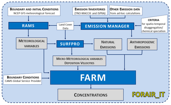
Figure 1.
Flowchart scheme of the FORAIR_IT model system.
The core of the modelling system is the chemical transport model Flexible Air Quality Regional Model (FARM) [37,38,39,40,41]. It is a three-dimensional offline Eulerian model that accounts for the transport, chemistry and removal of atmospheric pollutants. FARM’s major features include the handling of emission of pollutants from area and point sources, with plume rise calculation and mass assignment to vertical grid cells, three-dimensional transport by advection and turbulent diffusion, transformation of chemical species by gas-phase chemistry (SAPRC-99 [42]) and aerosol modules (AERO3 [43]), and the dry and wet removal of pollutants, depending on meteorology and land use.
Anthropogenic emissions come from the TNO-MACCIII emission inventory (Toegepast Natuurwetenschappelijk Onderzoek-Monitoring Atmospheric Composition and Climate III [44,45]) for the European domain. For the Italian domain, emissions are provided by the National Emission Inventories of Italy and neighbouring countries. Furthermore, particulate matter emissions from resuspension induced by road traffic and agricultural activities are calculated and included. Natural emissions are computed by the biogenic emission module MEGAN (Model of Emissions of Gases and Aerosols from Nature [46]) v2.04, integrated in SURFPRO (the diagnostic processor for micrometeorology); natural emissions include biogenic non-methane volatile organic compounds (NMVOCs), sea salt and crustal dust. Further details on emissions are available in [14].
The FORAIR_IT forecasting system is currently running with the non-hydrostatic prognostic model RAMS as meteorological driver. RAMS has been widely used since the 1990s for meteorological assessment and forecasting for CTMs in the USA [47,48,49,50], where it was developed, and outside the USA [51,52,53,54,55,56,57]. In FORAIR-IT, RAMS is run in a multiple-grid two-way nesting scheme. The horizontal resolution is the same as in the chemical transport model, while the vertical resolution is made of 35 levels. Convection is explicitly solved on the fine grid and parametrised on the coarse grid [58].
Together with meteorological variables, the CTM also needs, as inputs, micrometeorological and prognostic parameters like total and net solar radiation, snow, mixing height, albedo, roughness length, latent and sensible heat, wind stress, Monin–Obukhov length and turbulent diffusion coefficients. In FORAIR_IT, RAMS is coupled with FARM by means of the diagnostic processor for micrometeorology SURFPRO, which was originally developed to directly feed FARM, with the flexible ingestion of different types of measured or modelled meteorological data [22,59]. SURFPRO processes land use data, providing season-based information on surface physical features such as albedo, soil moisture, surface roughness, leaf area index and Bowen ratio. From the topography, season, latitude, cloud cover and solar constant, the incoming solar radiation Q (W m-2) is computed as a gridded 2D field, taking into account the presence of water bodies, terrain slopes and solar shading effects. In particular, net radiation and heat flux are computed according to the method in [60], as well as wind stress and Monin–Obukov length for unstable conditions. The latter two, for stable conditions, are computed according to [61]. Different formulations are available for the calculation of horizontal and vertical diffusion coefficients, the latter based on various boundary layer scaling regimes. The setup used in the standard configuration of FORAIR_IT uses a combination of local stability class/wind speed and stress tensor formulation from [62] for horizontal diffusion coefficients and the boundary layer parametrization regimes for vertical diffusion coefficients (mixing due to convection is not explicitly taken into account [63]). The schemes to compute Planetary Boundary Layer (PBL) scaling parameters are different for daytime (encroachment method, as in [64,65]) and night time (minimum value between [66] and [67]).
The work from [6] proved that the FORAIR_IT forecasting system produces results comparable with CAMS [18] across the European domain (daily mean PM10 and PM2.5 and daily maximum NO2 and O3). In particular, [6] outlined two crucial aspects: (i) by increasing the spatial model resolution in an area of interest, which, in the study, was Italy, lower values of Root Mean Square Error Difference (RMSED) can be obtained and (ii) the meteorological forcing may represent a key factor in explaining air pollutant concentration exceedances, in terms of both timing and intensities (in the study, PM10 was analysed).
2.2. WRF as Alternative Meteorological Driver
WRF is a mesoscale numerical weather prediction model. It was implemented in “Lambert Conformal” geographic projection at a horizontal resolution of 20 km over Europe and 4 km over Italy, in two-way nesting mode, and it was run non-hydrostatically on both grids with 34 unevenly distributed vertical levels reaching 5000 Pa. The first level is located at 25 m height and the first ten levels below are 1500 m height.
Boundary conditions came from the Global Forecast System (GFS) meteorological forecast of the National Centers for Environmental Prediction of the United States National Weather Service (NCEP), with a spatial resolution of 0.1°. The GFS fields at 18:00 UTC (Universal Time Coordinated) were used for initialising WRF. The first 6 hours were considered as a spin-up period for adjusting meteorological fields. The temporal output was obtained at hourly intervals.
The following combination of physical parameterisations (whose details can be found in references reported in the WRF documentation and user guide [25]), derived from the configuration adopted by the Developmental Testbed Center [68] and from literature studies focused on Italy [69,70,71,72,73,74], was tested as follows:
- Single-Moment 6 class scheme (WSM6) for microphysics;
- Rapid Radiative Transfer Model (RRTMG) for short- and long-wave radiation;
- MM5 (Fifth Generation NCAR/Penn State Mesoscale Model) scheme for surface layer;
- Noah Land Surface Model for land surface;
- Yonsei University scheme for Planetary Boundary Layer;
- Kain–Fritsch scheme for cumulus parameterization at 20 km resolution (turned off at 4 km resolution).
WRF could represent a potential improvement in the meteorological driving of our real-time air quality forecast system, given that it is fit for operational forecasting applications, with a higher computational efficiency compared to RAMS. This is partly due to the use of both shared and distributed memory parallel computing paradigms and partly to the possibility of using less accurate but more efficient parameterizations. For example, RAMS uses bin-emulating microphysics, while, in our configuration, WRF uses the WSM6 bulk parameterization scheme. This computational efficiency potentially represents a major upgrade for a daily operational forecast chain, given the limited time (a few hours) available for the simulation (download and preparation of input data, computation of 24–120 hourly multi-pollutant concentration fields, publication of results). Moreover, WRF has gained a leading position in the scientific community of air quality modellers, based on a pervasive use by U.S. scientists, including researchers of the national Environmental Protection Agency, and worldwide [75]. Such a wide user community provides, together with leading developers, continuous updates and support to users.
Lastly, while testing the effects of WRF implementation in FORAIR_IT, the feasibility of moving to a direct forcing of the CTM was tested as well; moreover, some micrometeorological quantities produced by the meteorological model were used directly in order to add physical consistency to the simulations. Indeed, SURFPRO was originally developed as micrometeorological pre-processor for FARM, regardless of the source of mesoscale meteorological variables (measured [22] or predicted by different weather models [59]). This is in line with many state-of-the-art air quality models, relying on standard meteorological observations and diagnostically estimated turbulence, atmospheric stability, mixing height, and dispersion coefficients. Off-line interfaces can limit the possibility of air quality models to access and exploit all the information provided by new-generation mesoscale meteorological models, while, at the same time, they can improve boundary layer description. A COST Action (COST728 [76]) explored, in detail, relevant European practices and advantages/shortcomings of using offline calculations for transport [77].
The abovementioned advantages in using WRF suggest that it should be tested to update the whole meteorological chain of prognosis and micrometeorology in FORAIR_IT.
2.3. FORAIR_IT Evaluation
FORAIR_IT forecasts were verified by considering the months of January and August 2019 as representative of winter and summer weather conditions, respectively.
2.3.1. Weather Conditions during the Selected Periods
In order to describe the average weather regime across Italy for the selected months, we looked at the NCEP/NCAR (National Centers for Environmental Prediction/National Center for Atmospheric Research) reanalysis fields at 2.5° resolution [78]. On average, January 2019 across Italy was characterised by low mean sea level pressure (mslp) at central and southern parts of the peninsula and cold air mass advection from northern and northeast Europe, driven by a high pressure ridge over the Atlantic up to the British Islands and western Scandinavia. This is clearly visible from the average fields depicted in Figure 2. Looking at anomaly fields computed across the 1981–2010 period (not shown here), in general, January 2019 for Italy was characterised by negative anomalies of temperature between 2 and 3 K as well as negative pressure and 500 hPa geopotential height (GPH) anomalies, denoting a period with the persistence of low pressure systems affecting mainly southern Italy, while this configuration the north of the country presented dry and cold conditions. On the contrary, August 2019 across Italy was dominated by moderately high pressure in the north, with the advection of hot air mass from Africa and high geopotential height values at 500 hPa. In this case, anomaly fields computed across the 1981–2010 period (not shown here) are characterised by above-average mslp and 500 hPa GPH, while temperature anomalies at 850 hPa reach values between 2 and 2.5 K all over the country, indicating hot and dry conditions affecting the area in August.
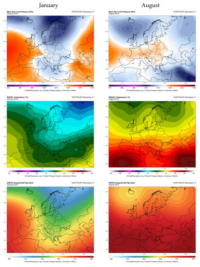
Figure 2.
Average fields of Mean Sea Level Pressure (hpa) (upper panel), 850 hPa temperature (midle panel) and 500 hPa (lower panel) geopotential height, respectively, for January (left) and August (right) 2019 derived from United States National Weather Service (NCEP)/NCAR Reanalysis. Image from [79].
2.3.2. Evaluation of Forecast Concentrations
Forecast concentrations of air pollutants regulated by the European Ambient Air Quality Directive [80] of major concern for human health in Italy [81] were evaluated in the present study, i.e., NO2 and O3. Observed concentrations at background monitoring stations for January and August 2019 were retrieved from near-real-time (NRT) data reported on an hourly basis to the European Environmental Agency (EEA, [82]) from Italy. PM10 and PM2.5 concentrations, despite being of major interest due to their high impact on human health in Italy [81], could not be evaluated because Italy only reported observed hourly values to the EEA on a few monitoring stations, which were not sufficient for a statistically significant model evaluation. NRT data cannot undergo full validation as they are reported to EEA immediately after measurement; therefore they can show anomalies and outliers.
For each station, the statistical consistency of hourly observed time series was checked, discarding stations with less than 75% of valid data on single days and with less than 75% of valid days in the month. Only the stations that satisfied the criteria for both months were considered valid in order to assure statistical consistency. The resulting number of NO2 monitoring stations was 136, with a total number of observations of 85,714 for January and 93,626 for and August. The number of O3 monitoring stations was 102, with a total number of observations of 63,270 for January and 71,484 for August.
In Table 1, the number of valid stations per pollutant and per type of area is shown, whereas the location of stations is visible in the Results section and in the complete list of stations reported in the Supplementary Materials.

Table 1.
Number and type of valid background stations used for the model evaluation.
Model concentrations evaluated in the study were referred to the first day of forecast concentrations. The model’s skill in reproducing NO2 and O3 observed concentrations, calculated separately for January and August 2019, was quantified by means of three statistical scores:
- Root Mean Square Error (RMSE), referring to hourly concentrations throughout the day and to the daily maximum of hourly concentrations. The value, expressed in µg/m3, is higher than or equal to zero by definition and the target value is zero (the lower the RMSE, the better the model performs);
- Correlation Coefficient (R), referring to hourly concentrations throughout the day. The non-dimensional value is between −1 and one by definition and the target value is one (the higher the R, the better the model performs);
- Modified Mean Bias (MMB), referring to hourly concentrations throughout the day. The non-dimensional value is between −2 and two and the target value is zero (the lower the absolute value of MMB, the better the model performs). Values lower than zero mean model underestimation, values higher than zero mean model overestimation. This indicator is often preferred to bias alone in evaluating model-based pollutant concentrations, because atmospheric species can vary greatly over time, space and evaluation metrics; therefore, a relative indicator ensures comparability between the performance of different species, and because it is symmetric, it therefore represents both underestimations and overestimations [83].
See Appendix A for details on the formulation of skill scores and Section 3 for a detailed explanation of the spatial and temporal reference of the sill scores.
2.4. WRF and RAMS Configuration Tests
For all WRF-driven tested configurations, basic meteorological variables produced by WRF were used: two-dimensional fields such as total cloud cover, sea surface temperature, total precipitation, snow depth, and three-dimensional fields such as meridional and zonal wind speed, vertical velocity, temperature, pressure, relative humidity and geopotential. Then, a scheme for sensitivity analysis was set up, starting with a baseline configuration (named S), with all micrometeorological variables (albedo, roughness length, soil heat flux, total and net radiation, sensible and latent heat flux, wind stress, Monin–Obukhov Length, PBL height and turbulent diffusion terms) calculated by SURFPRO. An additional configuration was used, i.e., the current FORAIR_IT set-up, with RAMS producing prognostic variables and SURFPRO in the S configuration. A total number of eight meteorological configurations were produced and are listed in Table 2.

Table 2.
Micrometeorological configurations for the sensitivity analysis. S is the baseline configuration with all micrometeorological variables produced by SURFace–atmosphere interface PROcessor (SURFPRO). S + variable is the configuration, where the variable is produced by the Weather Research and Forecasting Model (WRF), while the remaining micrometeorological variables are produced by SURFPRO.
In the experiment, for the configuration Snow, following the experience acquired during CAMS [18] where a simplified version of the snow cover computation proposed by [84] was tested, a snow mask was created, considering that all grid cells with a physical snow depth (SNOWH, variable in WRF, expressed in meters) higher than 1 mm were covered by snow, changing albedo, roughness length and Bowen ratio accordingly. All the other configurations were produced by changing, one by one, with the respective value calculated by WRF, a set of micrometeorological variables produced by SURFPRO: mixing height, albedo, roughness length, heat flux + friction velocity and Monin–Obukhov length. In the experiment, all includes the combination of all abovementioned variables computed by WRF at once.
The inclusion of the variables directly computed from WRF is coded by changing a simple “namelist” in the operational chain. The clear advantage is the simplicity of changing from one configuration to another. However, in terms of computational effort, even if each of the six WRF-based alternative configurations require a number of numerically solved operations lower than the Base configuration, the calculation time needed for one day of forecast is not sensitive to the different configurations, since it is mostly used by the two main models (WRF prognosis of mesoscale variables and FARM).
3. Results and Discussion
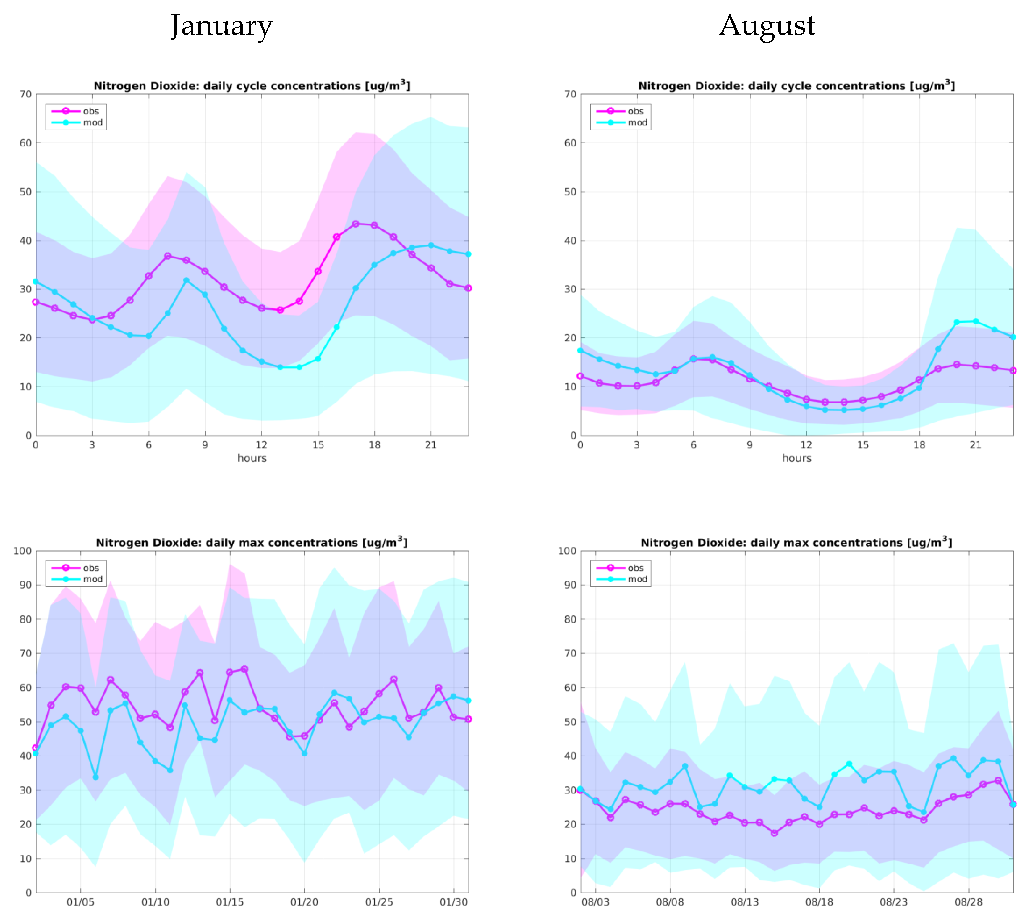
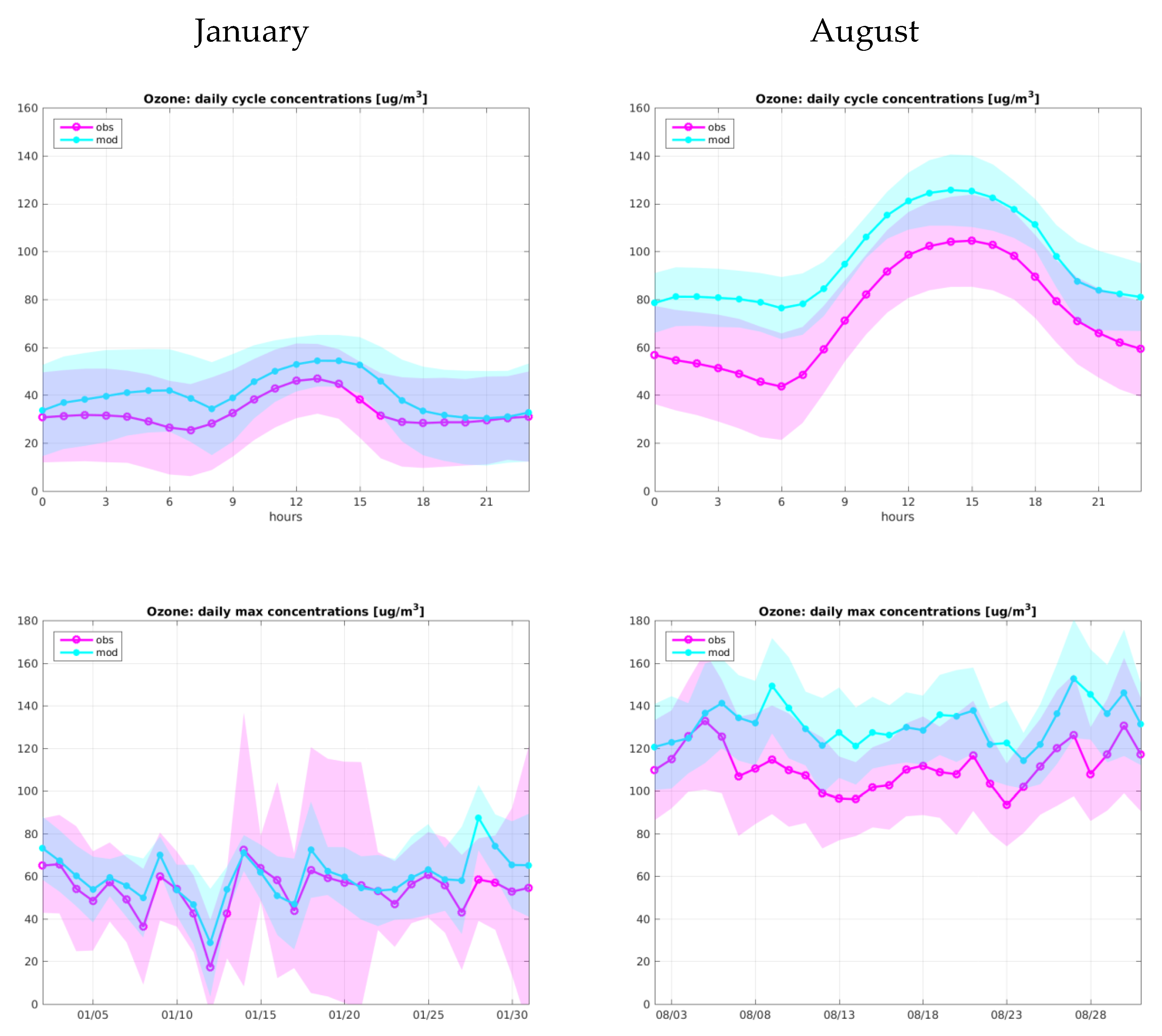
All model results presented below were extracted from the child domain at 4 km resolution. A first qualitative evaluation of model performance is provided by looking at the average daily cycle of hourly concentrations and the average daily maximum of hourly concentrations, produced in the Base configuration. The times all refer to UTC. Here, observations and simulated values were compared at the locations of monitoring stations (simulated values were extracted by means of nearest neighbour interpolation). Figure 3 and Figure 4 show a comparison for NO2 and O3, respectively, for January and August 2019.
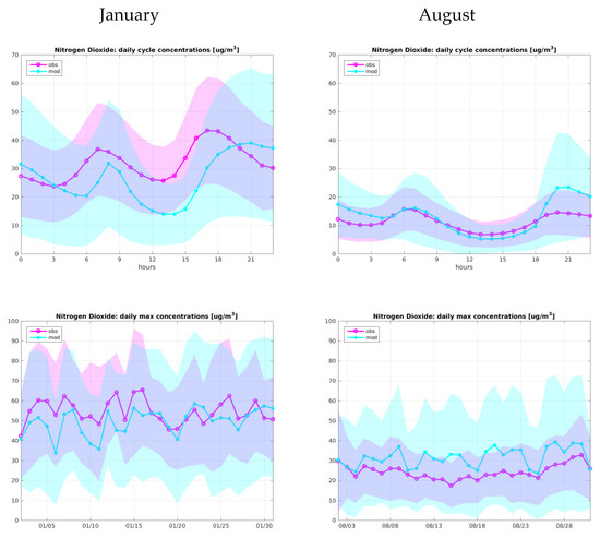
Figure 3.
NO2—observed (violet) and modelled (light blue) average daily cycle of hourly concentrations (upper panel) and average daily maximum of hourly concentrations (lower panel), for January (left) and August (right). The dotted line is the average on all stations, the coloured strip is in the range of the 25th–75th percentiles of the values at stations. The x-axis reports UTC times.
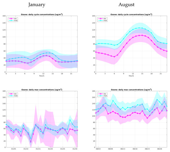
Figure 4.
O3—observed (violet) and modelled (light blue) average daily cycle of hourly concentrations (upper panel) and average daily maximum of hourly concentrations (lower panel), for January (left) and August (right). The dotted line is the average on all stations, coloured strip is in the range of the 25th–75th percentiles of the values at stations. The x-axis reports UTC times.
Figure 3 and Figure 4 highlight the average value and the range between the 25th and 75th percentile values, calculated at all stations. For NO2, the daily cycle of average hourly concentrations is in better agreement with the observations in August than in January. In general, the lack of spatial resolution leads to underestimated model values (see comments to Figure 5). For the all-station average, in January, the model gives an underestimation in daytime and a slight overestimation at night. In August, the model gives good results in daytime and an overestimation at night. Thus, there could be a systematic underestimation of night time mixing height, which is more pronounced in August. This would compensate underestimations in concentrations in January and lead to August overestimation during the night. As for daytime bias, which is present in January and absent in August, this is probably partly due to the underestimation of emissions (see description of Figure 5), which is more significant in January when emissions are higher.
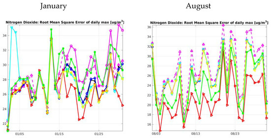

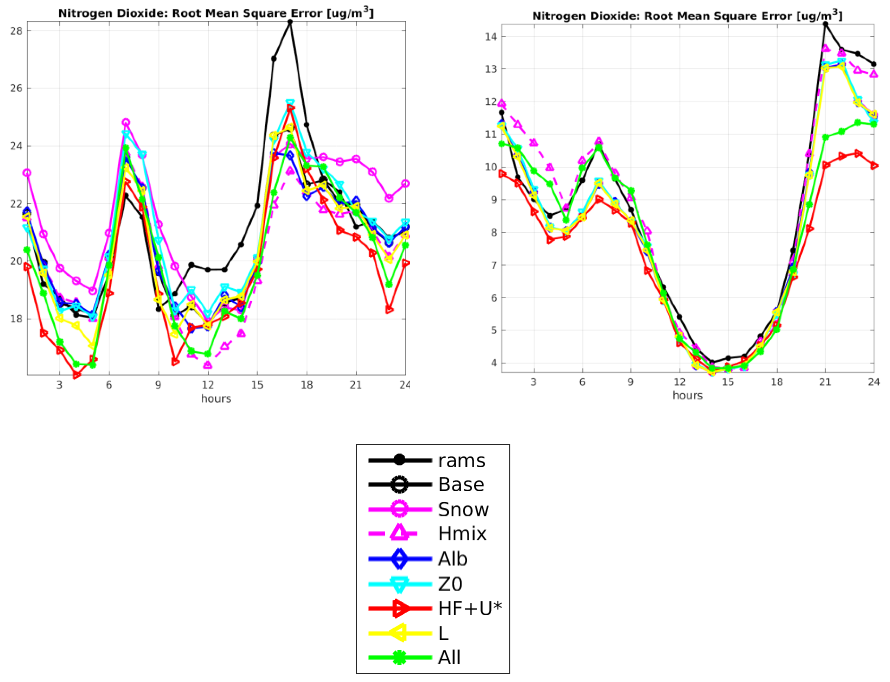
Figure 5.
NO2—RMSE of the daily maximum of hourly concentrations (upper panel) and of hourly concentrations (lower panel), for January (left) and August (right). The x-axis reports UTC times.
Ozone is generally overestimated (slightly in January, more significantly in August). For both the pollutants, daily maxima concentrations are quite well reproduced in January (except for the underestimation of NO2 during the first half of the month), while in August a general overestimation of simulated values is present, which is more significant for O3. The spatial variability (represented by the width of the range of the 25th–75th percentiles) of O3 is well captured by the model, both on a daily and an hourly basis, while for NO2 it is, in general, overestimated, especially in August during night time.
In the following Section 3.1 (NO2) and Section 3.2 (O3), the results are shown and commented on, for each pollutant, following this order:
- RMSE, R and MMB, synthesizing all valid monitoring stations and all the hours of the whole month;
- RMSE of the daily maximum of hourly concentrations, synthesizing all valid monitoring stations for each day of the month, and RMSE of hourly concentrations, synthesizing all valid monitoring stations and all days of the month for each hour of the daily cycle;
- R and MMB of hourly concentrations, synthesizing all valid monitoring stations and all days of the month for each hour of the daily cycle;
- Maps of the monthly average field of model concentrations, overlaid by monthly model skills on single monitoring stations.
3.1. NO2
Table 3 shows that the RMSE of January is similar for all configurations, between 22.3 µg/m3 (for Heat Flux and Wind Stress (HF+U*), slightly improving the Base simulation) and 24.7 µg/m3 (for Snow). R is substantially the same for all configurations (around 0.56). The MMB is between −0.29 and 0.4, with all configurations being better or equal to the Base, except for HF+U*, scoring 0.4. August outcomes confirm the stability of RMSE among the different configurations, around 13.7 µg/m3, with HF+U* showing the best skill (12.2 µg/m3, the only improving the Base simulation) and Mixing Height (Hmix) the worst (15.3 µg/m3). R is around 0.42 for all configurations apart from Hmix and HF+U*, slightly higher than the Base case. The MMB is close to zero in all cases. Apart from slight differences on single scores, HF+U* and Hmix register the most uniform improvements with respect to Base.

Table 3.
NO2—monthly Root Mean Square Error (RMSE) (µg/m3), Correlation Coefficient (R) and Modified Mean Bias (MMB). Values in bold indicate that performance improved (lower RMSE and MMB, higher R) with respect to the Base configuration.
The All configuration shows the best performance of the other configurations (even with a slight increase in R in August), improving Base as well.
RAMS has significantly lower correlations, indicating an inferior capability in reproducing the variability of monthly concentrations and a lower MMB (indicating higher underestimation) in August. The remaining scores are comparable to WRF-driven values.
The simulation system in all configurations gives a higher R in January and MMB values closer to zero in August, suggesting that in winter, when concentrations are higher, the absolute values are underestimated, but the variability of concentrations is better reproduced than in summer. The negative bias in both months suggests a systematic underestimation of NOx in the emission inventory, while the larger bias in January may be related to an inaccurate monthly emissions profile. The RMSE has higher values in January rather than in August, because a score like RMSE, which is not normalised, is proportional to concentration values. Therefore, the model chain behaves better in January than in August, which is a desirable outcome, given that the overall aim is to reproduce, at best, the high concentrations recorded in wintertime (when emissions and atmospheric stability are higher and the PBL height is generally lower), represented here by the month of January.
In the plot of the RMSE of the daily maximum of hourly concentrations, in both months (Figure 5, upper panel), all configurations show a large variability. Values range in January from 22 to 36 µg/m3, with the maximum value being reached on the 13th, before and after the sharpest variations in the month. This instability is also visible in absolute concentrations in Figure 3 (lower right panel): here, on the 6th and the 13th of January, observed and model values show the largest bias in the month, but the 6th shows a local minimum for the series, while from the 12th to 14th the series display different patterns. Excluding an inaccurate simulation of meteorology for the 13th (as the lower panel in Figure 4 shows, for the same day, a good agreement with O3 observations), a possible explanation is an outlier in the observed values at one or more stations. In August, the variability is from 15 to 36 µg/m3. From 1st to 14th January, all configurations show similar values, around 24–28 µg/m3, apart from Z0 on the 2nd and the 3rd, then HF+U* tends to decrease and Hmix tends to increase, with respect to the other configurations, which maintain quite similar values and trends. In August, HF+U* confirms to be the best configuration, while the other ones do not show significant differences, apart a slight worsening of Hmix.
Regarding the RMSE of hourly concentrations (Figure 5, lower panel), values are significantly higher in January (17–26 µg/m3), than in August (4–13 µg/m3), due to the larger value of wintertime concentrations. In January, values are proportional to hourly concentrations, with peaks in early morning and late afternoon and minimums at night and around midday. A first explanation could be the an underestimation of road traffic emissions during rush hours, known to be an issue affecting emission inventories, both for underestimations of real-world emission factors used in the calculations and for approximations in the hourly allocation of aggregate yearly emissions [85]. A second reason is probably the lack of spatial resolution in the CTM, which is a well-known problem in regional-scale simulations, affecting NO2 more than other pollutants due to the high sub-grid spatial variability of emissions, which is lost during spatialization on model grids with kilometric-scale spacing [86,87,88]. HF+U* is, again, the best configuration from 1.00 to 10.00 and from 21.00 to 24.00, but Hmix has the lowest values from 11.00 to 17.00. During August, all configurations have very similar values, with a clear U-shaped curve from 7.00 to 21.00, with HF+U* performing best and Hmix performing worst. The overall hourly pattern is not really different between January and August, even if August has lower daily variability.
R (Figure 6, upper panel) has low values on average, ranging from 0.25 to 0.5 in January and from 0.15 to 0.45 in August. In January, Z0 performs worst, HF+U* has the highest values from 1.00 to 10.00 and from 19.00 to 24.00, Hmix is the best configuration from 11.00 to 18.00. In August, very similar values are obtained among the configurations, with HF+U* and Hmix slightly better particularly from 13.00 to 20.00. The overall daily pattern shows increasing values in the first 13 hours and decreasing values afterwards in both months, with some exceptions such as the local minimum at 7.00 and the local maximum at 17.00 in January.
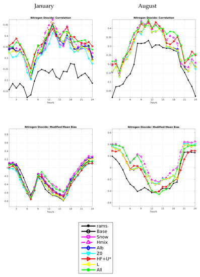
Figure 6.
NO2—R of hourly concentrations (upper panel), MMB of hourly concentrations (lower panel), for January (left) and August (right). The x-axis reports UTC times.
The MMB (Figure 6, lower panel) shows a systematic underestimation in January, apart from hours 1.00 to 2.00 and 22.00 to 24.00, with the highest absolute errors at 7.00 and 16.00. All configurations give similar results, with Hmix showing slightly lower underestimation from 11.00 to 16.00. In August, both overestimation (night time, from 1.00 to 5.00 and from 20.00 to 24.00) and underestimation (from 10.00 to 19.00) are recorded for almost all configurations. Again, Hmix and HF+U* can be clearly distinguished by the others. The former is the worst from 1.00 to 10.00 and from 20.00 to 24.00, and the best from 11.00 to 19.00. The latter shows the highest underestimation from 10.00 to 19.00, but the lowest overestimation from 21.00 to 24.00.
All plots of Figure 5 and Figure 6 indicate that, unsurprisingly, the All configuration shows values which are either similar to one configuration or intermediate between configurations, depending on which is the prevalent effect of single micrometeorological parameters in the All simulation. Over several days (first half of August for RMSE of daily maximum) and hours (night and midday for January RMSE, afternoon and evening for R), All “follows” either HF+U* or Hmix in giving better performances.
As for RAMS, the RMSE of daily maximum and of hourly concentrations is hardly distinguishable from WRF configurations, except for the hours from 11.00 to 18.00 in January, when it is visibly the highest. Correlations are always significantly lower than WRF. The MMB of January and of the second half of a typical day in August is similar to WRF, while the values are visibly lower in August from 1.00 to 4.00 (improving WRF bias) and from 5.00 to 11.00 (worsening WRF underestimation).
The overall picture emerging from the analysed skill scores of January is clearly a better performance of HF+U* during night time and of Hmix during daytime. August partially confirms the better results of HF+U*, on RMSE and R, while the MMB quality is strongly dependent on the hour of the day. August Hmix has variable rankings, being the worst for RMSE and night time MMB, and the best for R and daytime MMB.
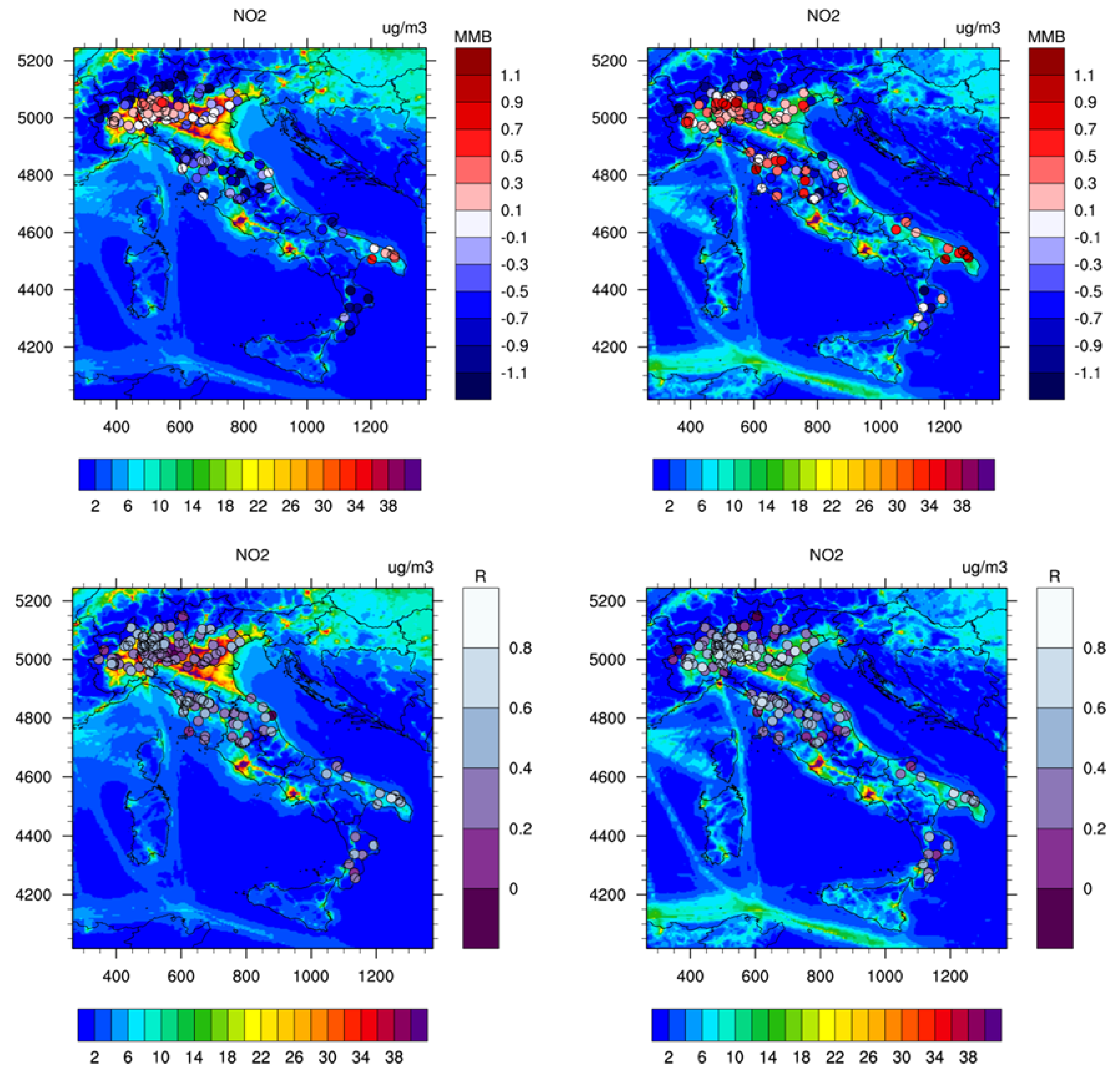
The model’s performance for single monitoring stations is presented in Figure 7 for the two relative scores (R and MMB) in the Base configuration, superimposed with the monthly average of model concentrations. R and MMB were chosen because the RMSE is dominated by large values due to the squaring operation in the calculation formula. Having used NRT observations, which are not quality-controlled, outliers could alter the RMSE in some stations, while it is less probable that the all-station averages presented above are significantly modified by observation anomalies on single stations.
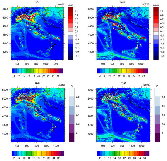
Figure 7.
NO2—Monthly average of model concentrations of January (left) and August (right) for the WRF Base configuration, overlaid with monthly values of MMB (upper panel) and R (lower panel) at monitoring stations. Model concentrations have a horizontal colour bar (µg/m3), skill scores have a vertical colour bar (non-dimensional).
The spatial distribution of pollutant concentrations is consistent with previous studies on Italy (e.g., [14]), showing a large NO2-polluted area in the north (Po Valley) with clear hotspots over cities and along the main roads. The MMB calculated at the measuring stations is generally good (between −0.7 and 0.5); in January, there was no clear dependency on the location of the stations, while, in August, which is indicative of summertime, higher values are obtained in urban areas of the Po Valley and Central Italy, and performances over the Apulia region (southeastern area) are generally lower. R is generally higher in August, without a clear geographical distribution. Both in January and in August, values are lower with respect to O3 (presented in the next sub-section); however, the sharp spatial gradients, typical of NO2 concentrations, pose a challenge to regional air quality modelling systems in capturing the time variability observed at measuring stations, since a shift of few kilometers in the meteorological and concentration field patterns may lead to a completely different temporal variability of modelled concentrations. Moreover, factors in the weather fields such as initial/boundary conditions, parameterizations choice can positively affect the meteorological simulations and possibly the air quality fields. In this respect, sensitivity tests would be needed, which are not the focus of the current work.
The exact values of monthly R and MMB, as well as those of monthly RMSE, at each monitoring station are reported in the Supplementary Materials.
3.2. O3
Table 4 shows that in January, on average, all configurations have similar values of RMSE, around 30–32 µg/m3, and of R, about 0.45, while the MMB ranges from 0.05 (Hmix) to 0.18 (Snow), with Hmix, HF+U*, Alb and All performing better than the Base configuration. In August, the RMSE is around 35.5 µg/m3 for most configurations, except for Hmix (33.1 µg/m3), HF+U* (33.5 µg/m3) and This shows the lowest value for WRF (31.5), both improving the Base simulation. R is around 0.64 for all configurations except for All that shows the best score (0.67), while MMB is between 0.28 and 0.35, with Hmix, HF+U*, L and All performing better than the Base configuration.

Table 4.
O3—monthly RMSE (µg/m3), R and MMB. Values in bold indicate performance improved (lower RMSE and MMB, higher R) with respect to the Base configuration.
The All configuration shows the best performance out of the other configurations, with several improvements (January MMB, all scores in August), resulting therefore the best WRF-driven set-up.
RAMS, though improving WRF-based RMSE and MMB, has significantly lower correlations for NO2. The results of the two pollutants are probably covariant, i.e., the misrepresentation of the variability of NO2 monthly concentrations is reflected in O3.
The simulations show contrasting seasonal skills for R (higher in summer) and MMB (closer to zero in winter). Therefore, a consideration can be derived that is similar to NO2, i.e., that in the months of higher concentrations, the model has biased absolute values (overestimated in summer for O3, while they are underestimated in winter for NO2), but a better capacity to capture the variability of concentrations compared to the months of lower concentrations.
In the end, All, Hmix and HF+U* are the best performing configurations, improving five out of six monthly skill scores. Regarding HF+U*, its good monthly performance in detecting NO2 is confirmed for O3, therefore suggesting that the updated and detailed physics in WRF (MM5 surface layer scheme for U* and Noah land surface model for HF) are more precise than SURFPRO parameterisations [60] in describing surface fluxes in the different seasons. As for Hmix, with respect to the other configurations, O3 performs better than NO2, therefore it is more sensitive to the change of mixing height from SURFPRO to WRF. A possible reason is the different vertical distribution of the two pollutants: while NO2 largely comes from primary emissions of NOx, therefore being more concentrated at ground level, O3 is secondarily produced in the atmosphere at different heights and can be more concentrated at higher altitudes [89]. This would confirm that WRF reproduces its results better the vertical transport inside the boundary layer.
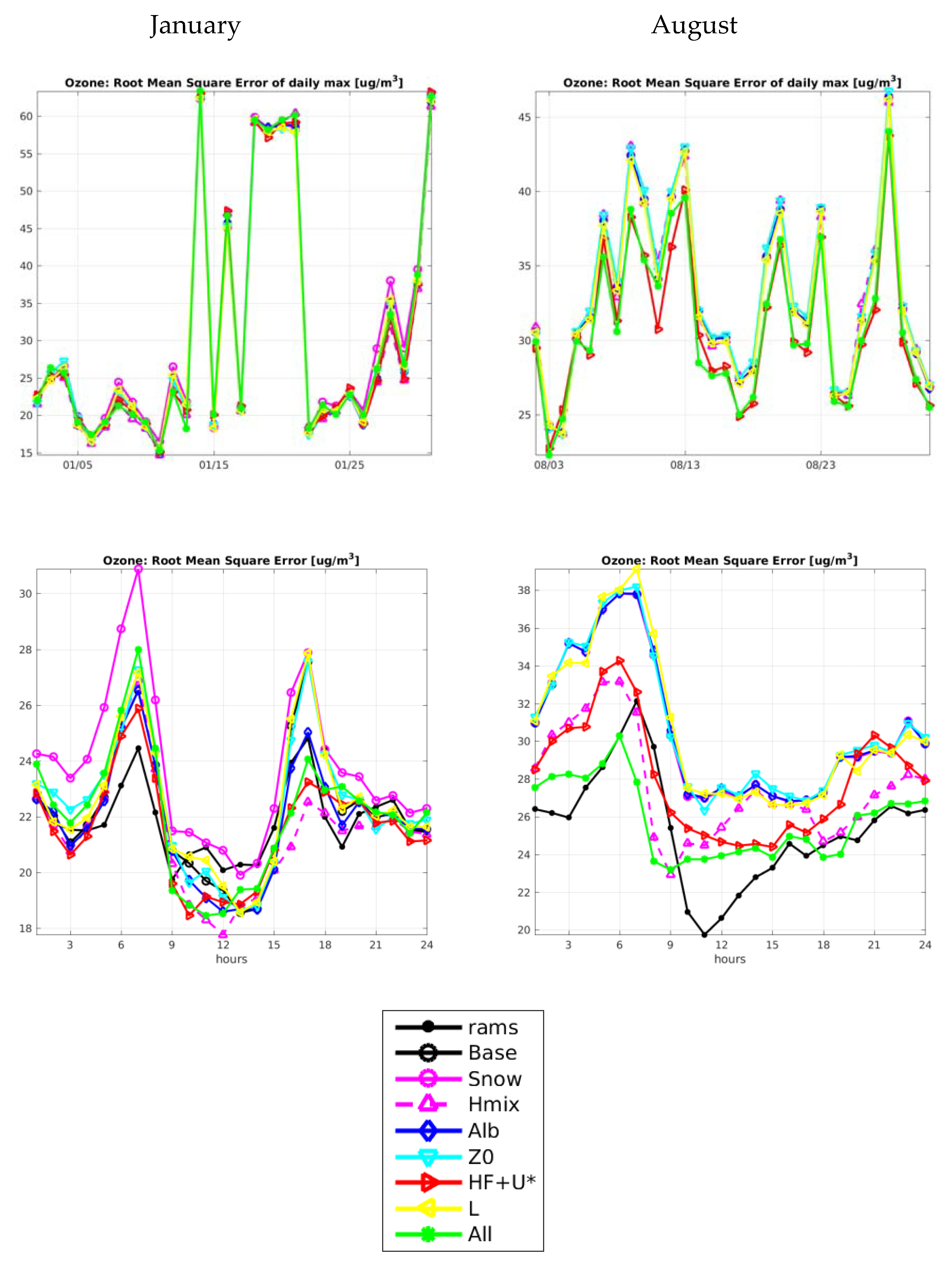
In the plot of the RMSE of the daily maximum of hourly concentrations (Figure 8, upper panel), reasonable values are obtained in January from the 1st to the 13th, ranging from 15 to 27 µg/m3, and from the 22nd to the 30th, ranging from 19 to 40 µg/m3, with a local maximum on the 28th. Then, higher values (around 62 µg/m3) are recorded on the 31st, possibly due to an increase in concentrations started the day before, but the observation anomaly is not excluded. Instead, no straightforward quality assessment of observed values is possible from the 14th to the 21st, due to the sharp variations in RMSE in the first four days and to the substantial persistence of very high values, around 60 µg/m3, in the last four days. This could be a high concentration episode, starting on the 15th (which could be an outlier) or even on the 14th (which could be a valid value) and ending on the 21st, or conversely a period of multiple observation anomalies. This hypothesis is supported by the much higher variability in observations recorded exactly on the mentioned days (14th, 16th, 18th–21st, 31st, Figure 4, lower panel). Despite the general good agreement between the spatial variability of observations and the simulation in January, as shown by the 25th–75th percentile ranges in Figure 4, in the period of the 14th–21st the variability is higher in the observations than in the model, suggesting that, even if a high concentration episode had occurred, it would have been quite localised. All configurations have very similar values. In August, no clear outliers are visible and the variability is from 23 to 47 µg/m3, with significant yet reasonable inter-day variations. HF+U* performs slightly better than the other configurations.
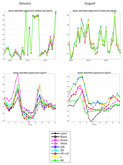
Figure 8.
O3—RMSE of the daily maximum of hourly concentrations (upper panel) and of hourly concentrations (lower panel), for January (left) and August (right). The x-axis reports UTC times.
The RMSE of hourly concentrations (Figure 8, lower panel) ranges from 19 to 34 µg/m3 in January and from 22 to 40 µg/m3 in August, indicating that model performances have similar hourly variability in the two months, despite the higher concentration values in August. In January, RMSE values are in counterphase compared to hourly concentrations of Figure 4 (upper panel), with peaks at 7.00 and in early afternoon and a minimum plateau around midday, like for NO2. This seems to indicate that, regardless the pollutant, in January the model performs better in the central hours of the day and of the night, with a degradation in its skill in the transition hours. This could be due to the hypothesised underestimation of NOx emissions during peak traffic hours, leading to lower concentrations of NO2 and lower titration of O3. Hmix performs slightly better from 10.00 to 20.00, like NO2, but for a longer time interval, while Snow has higher errors in most hours of the day, again confirming the NO2 results. In August, the peak values in early morning cover the interval between 5.00 and 7.00 (one hour before NO2 morning peak values), then most models show a U-shaped pattern like for NO2, but with a lower rate of increase after the minimum value around 15.00. Hmix and HF+U* can be distinguished from the other configurations: HF+U* follows the general daily cycle (apart from slight differences from 19.00 to 24.00), but shows lower values in most hours of the day, while Hmix shows the absolute minimum value of all plotted hourly RMSE at 9.00, then an increase in the morning is observed followed by a decrease in the afternoon, and finally an ascending ramp in the last hours of the day, like most of the other configurations. Values are lower in daytime from 10.00 to 18.00.
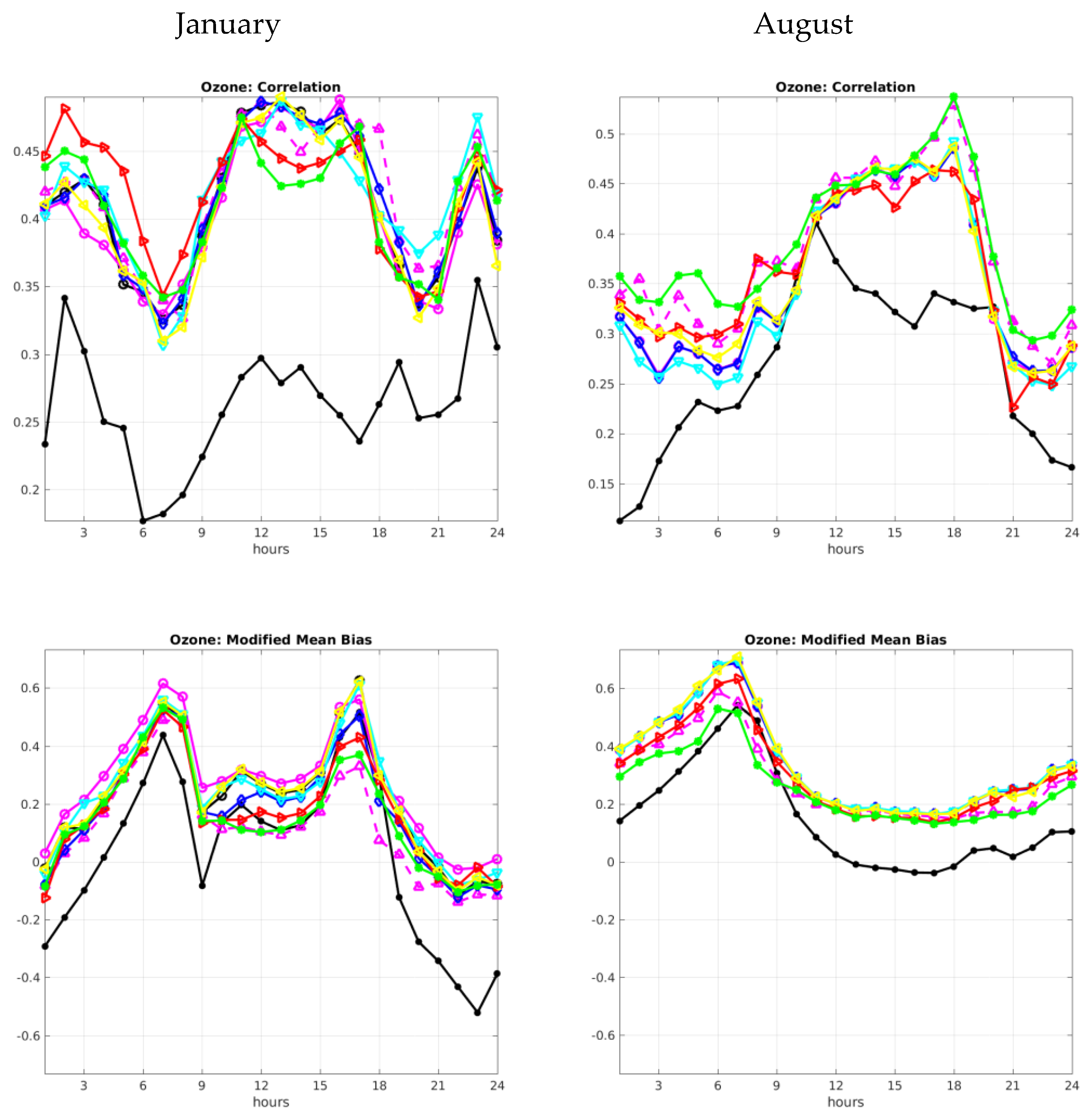
Values of R (Figure 9, upper panel) are between 0.24 and 0.44 in January and between 0.23 and 0.52 in August. In January, the average pattern is a W-shape, it shows descending values at night, with the absolute minimum between 7.00 and 8.00, then a sharp rise until 11.00, followed by a decrease towards a relative minimum value at 21.00, then, again, a rapid increase, until 23.00. HF+U* is the best configuration during night time, Hmix has the highest values from 10.00 to 20.00, Z0 gives the best results at 21.00 and 22.00. August values show a different pattern, with lower values at night (with Hmix slightly better) and higher values during the day (Hmix is the best from 7.00 to 8.00, together with HF+U*, and from 17.00 to 20.00).
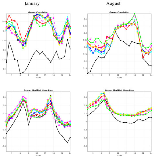

Figure 9.
O3—R of hourly concentrations (upper panel), MMB of hourly concentrations (lower panel), for January (left column) and August (right column). The x-axis reports UTC times.
The MMB values Figure 9, lower panel) indicate good performances in January, between –0.2 and 0.2 in most hours of the day, while from 5.00 to 8.00 and from 16.00 to 17.00 the overestimation is higher. While the RMSE only indicates that the model performs better in the central hours of the day and of the night, the MMB reveals that NO2 is underestimated and O3 is overestimated, with higher absolute MMB values in the transition hours. This suggests that one of the possible interpretations given above for NO2 and RMSE of O3, i.e., a likely underestimation of NOx emissions during peak traffic hours, could be confirmed, thus leading to lower concentrations of NO2 and lower titration of O3. Hmix configuration is better from midday to 20.00. Later in the day, it gives larger underestimation at 21.00 and 22.00. In August, the absolute maximum is recorded at 6.00 or 7.00 depending on the configuration. Afterwards, the score quickly declines and remains quite stable between 10.00 and midnight. There is not a clear ranking of performances among the different configurations.
Like for NO2, Figure 8 and Figure 9 show that the All configuration tends to follow either one configuration (when the influence of the relevant parameter is higher) or intermediate values between configurations. Nevertheless, there are exceptions, with All clearly scoring the best values. This is the case for the August night time hours, probably due to a synergistic effect of HF+U* and Hmix in producing a less diffusive PBL, thus limiting the overestimation and slightly increasing the correlations.
As for RAMS, the RMSE of daily maximum is not distinguishable from WRF configurations. The RMSE of hourly concentrations is lower than WRF in early morning in January and in the night and midday hours of August. Correlations are almost always significantly lower than WRF, as with NO2. The MMB indicates a smaller overestimation than WRF in January from 1.00 to 9.00 and from 19.00 to 24.00, while, in August, a reduced overestimation can be found for the whole day. It is therefore clear that WRF has added more consistency in describing the variability, while RAMS–SURFPRO is still better in representing the mass of generated pollutant, probably due to a better calculation in RAMS of variables input to SURFPRO, such as solar radiation (during the day) and PBL (at night). Therefore, further work will be needed to evaluate other WRF micrometeorological parameters, namely solar radiation and the eddy turbulent diffusion coefficients.
In general, in January, all configurations show better performances during daytime. In August, similar features are obtained, with most daytime hours showing better scores, apart from early morning, when performances are worse. All, Hmix and HF+U* present the best overall results.
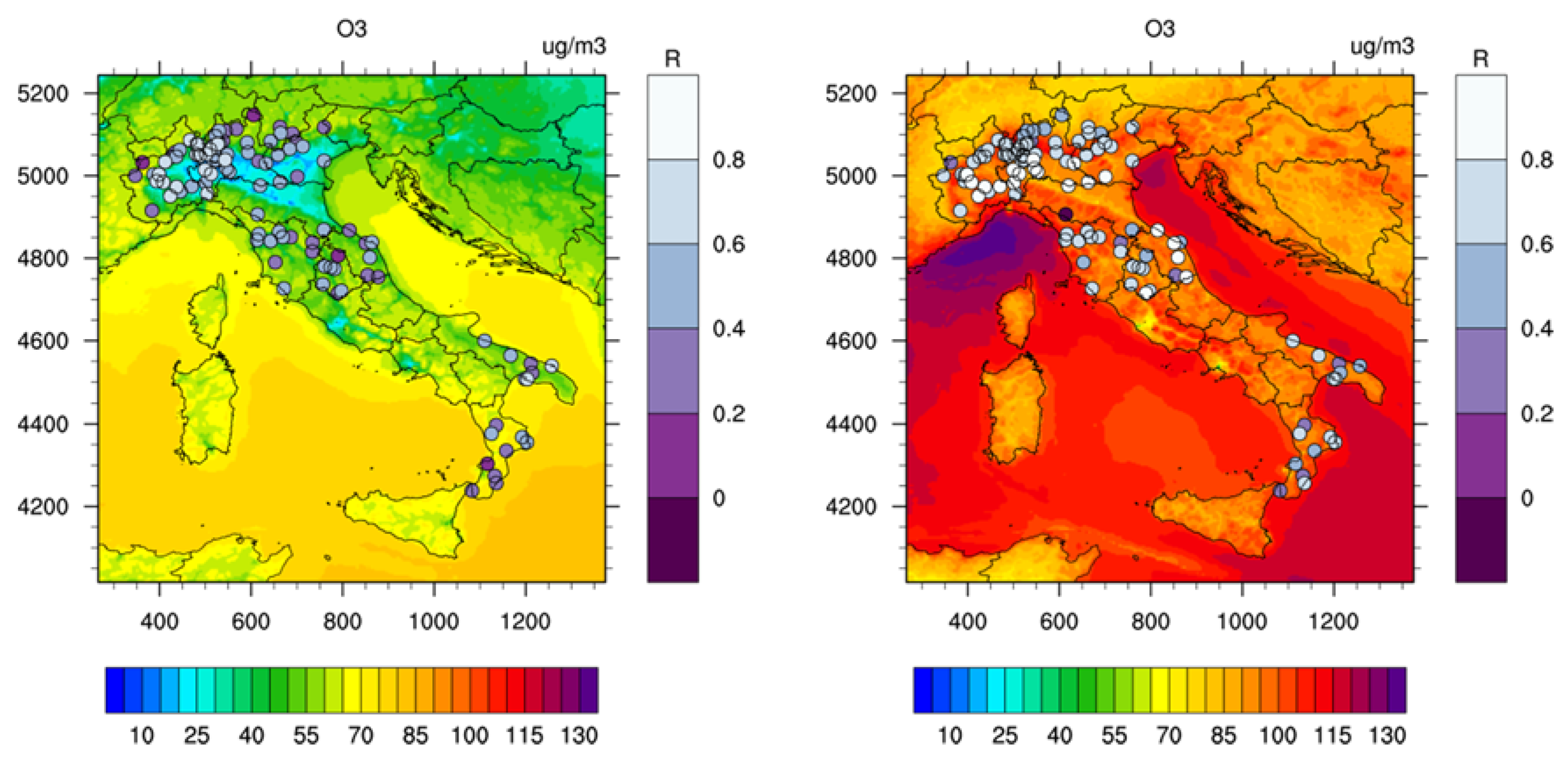
As for NO2, the model performances for O3 on single monitoring stations are presented in Figure 10, superimposed with the monthly average of model concentrations for the two months and the two skill scores, as explained in Section 3.1.


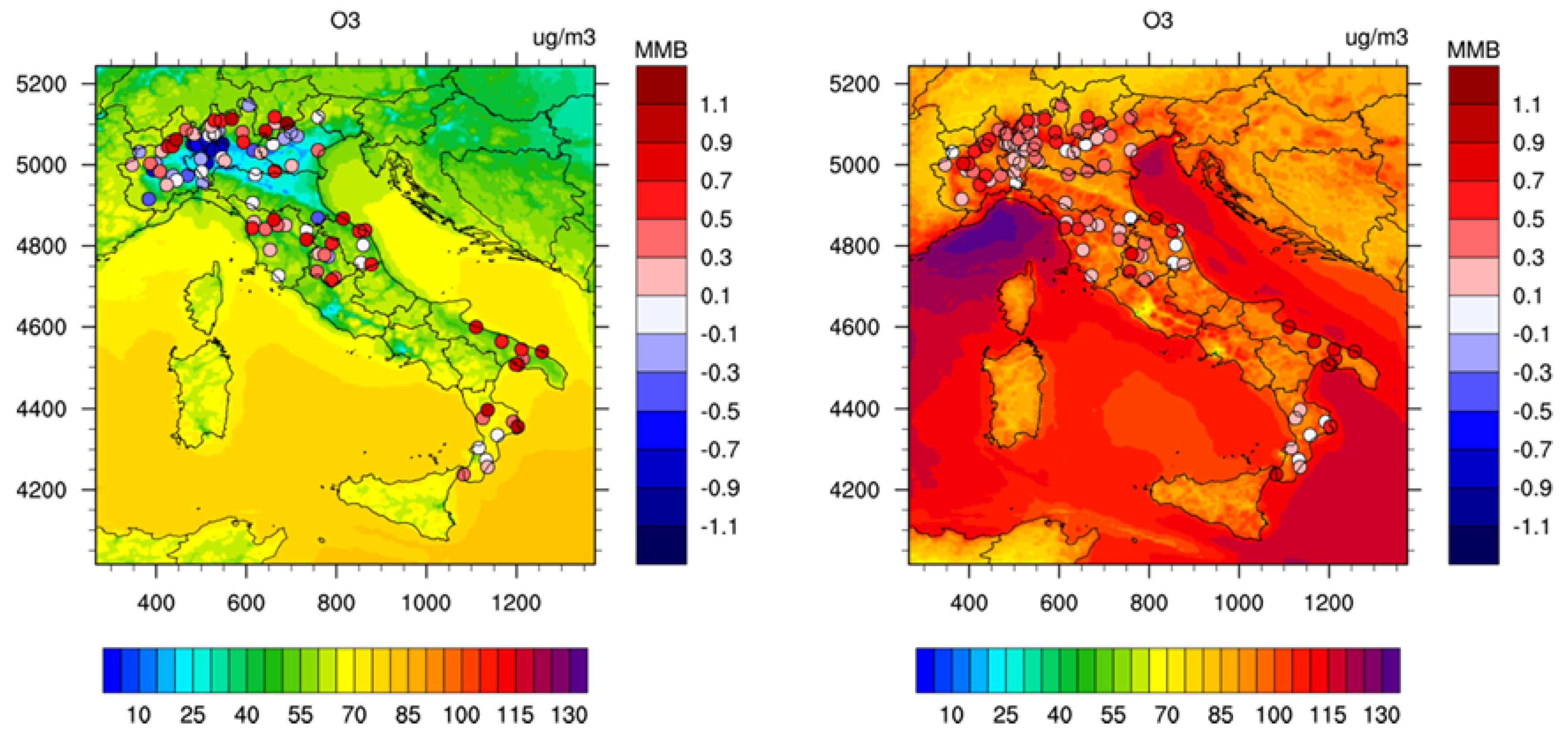
Figure 10.
O3—Monthly average of model concentrations of January (left) and August right) for the Base configuration, overlaid with monthly values of MMB (upper panel) and R (lower panel) at monitoring stations. Model concentrations have a horizontal colour bar (µg/m3), skill scores have a vertical colour bar (non-dimensional).
In January, over-land concentrations are clearly inversely related to NO2 concentrations, with minimums in the largest urban areas and regional areas of maxima in Southern Italy, while offshore concentrations are generally higher than those over land and are driven by southern boundary contributions. High levels of O3 in August are more uniformly recorded over the peninsula, particularly along the coastlines, where the contribution of transport from the sea is important. In contrast to January, the maximum values (over 130 µg/m3) are in the violet “stain” visible on the Ligurian sea, likely due to transport from the Eastern Mediterranean sea (the maximum level along the borders of the modelling domain is reached, between 120 and 125 µg/m3, about 100 km southwest of the Ligurian sea). Both skill indicators show a better model performance in the Po Valley and (in August) in Central Italy, whereas the pre-alpine region, Southern Italy and (in January) Central Italy score higher MMB and lower R values.
The exact values of monthly R and MMB, as well as those of monthly RMSE, at each monitoring station are reported in the Supplementary Materials.
4. Conclusions
In the process of the implementation of the full operational mode of the FORAIR_IT real-time air quality forecasting system over Italy on a daily basis, the WRF model was initially tested as meteorological driver for the chemical transport model (CTM) core (FARM) of the system, as an alternative to RAMS, currently embedded in the system. WRF was used for the production of the meteorological variables at the regional scale and then tested in seven different configurations for the simulation of the micrometeorological variables input to FARM. In each configuration, all micrometeorological variables were produced by SURFPRO, apart from one produced by WRF: snow, mixing height, albedo, roughness length, soil heat flux + friction velocity and Monin–Obukhov length. Results produced by RAMS with SURFPRO were also included in the study. One-day forecast concentrations from January and August 2019 were compared to near-real-time observations to assess the model performance by means of three skill scores (Root Mean Square Error (RMSE), Correlation Coefficient (R), Modified Mean Bias (MMB)).
The working hypothesis that drove the present work, by strengthening the coupling between meteorological conditions and the pollutant concentrations, was to increase the physical consistency between mesoscale and micro-meteorological variables, in order to capture the high-concentration events mainly driven by the meteorological conditions. With that in mind, the use of WRF variables to directly feed FARM simulations would be preferable, if the results do not show excessive degradation when compared to the Base configuration, i.e., using SURFPRO as a different micrometeorology processor.
We highlight the following key findings:
- WRF significantly improves RAMS-driven results on R, indicating its higher capability in reproducing the spatial and temporal variability of concentrations. This is the first confirmation of the potential for improvement by using WRF in FORAIR_IT;
- The results of the Base WRF-driven simulation compared to the observed values show that the model performs better in January with respect to August for NO2, while the opposite is true for O3. The daily cycle of average hourly concentrations of NO2 in January is underestimated in daytime and well reproduced during night time, and it is generally well reproduced in August. The daily cycle of O3 is generally overestimated in both months. Daily maxima concentrations of both pollutants are quite well reproduced in January, apart from some underestimation of NO2 in the first half of the month, and overestimation in August. The picture (underestimation of NO2, overestimation of O3) seems to confirm a common finding in regional-scale CTM simulations, with several explanations (underestimation of road traffic emissions, lack of spatial resolution);
- Monthly scores showed that a general improvement is obtained by directly using the Heat Flux and Wind Stress (HF+U*) and the Mixing Height (Hmix) estimated by WRF, for both the analysed pollutants. The All configuration shows the best performance out of the other configurations, with several improvements on O3. HF+U* is improved by physics in WRF (MM5 surface layer scheme for U* and Noah land surface model for HF), while Hmix gives a larger improvement to O3, likely due to the better representation of PBL vertical mixing in WRF. RAMS has significantly lower correlations, indicating an inferior capability in reproducing the spatial variability in monthly concentrations, and lower MMB on O3, probably due to more accurate solar radiation enhancing the photochemical generation of the pollutant;
- Concerning the time variability of the statistical scores, in terms of both intra-day variability and daily cycle variability, all the experiments show similar features, suggesting that the introduction of new meteorological variables into the CTM do not significantly change the time variability of the concentrations for both pollutants and months. For NO2, both in January and in August, HF+U* and Hmix score the best results in most (but not all) hours of the day. For O3, both in January and in August, all configurations show better performances in daytime (apart early morning in August), with Hmix and HF+U* presenting the best overall results. As with the monthly scores, the All configuration shows the best performance out of the two mentioned configurations and shows further improvements in August night time hours, probably due to better PBL stability. RAMS has, again, significantly lower correlations and hence worse skills in following the variability; however, it has lower O3 MMB values, namely in January night time (due to better PBL stability) and all hours during a typical August day (confirming the better solar radiation and indicating that this will be a key parameter to be taken from WRF and tested in future analyses);
- The spatial distribution of performance skill scores (MMB and R) calculated at monitoring stations for the Base configuration did not show a clear variability with the location. For NO2 in August, both MMB and R are slightly higher in urban areas of the Po Valley and Central Italy, suggesting that, for these stations, a better description of time variability and a lower quality of local emission input, with respect to the remaining stations. Conversely, for O3, both performance skill scores indicate better results in the Po Valley and (in August) in Central Italy, whereas the pre-alpine region, Southern Italy and (in January) Central Italy score higher MMB and lower R values.
While the statistical significance of the hourly analysis on a typical day of each studied month is quite robust, the limited number of months in the analysed year prevents us from reaching statistical significance on monthly and annual performance. This is a limitation of the present work. Moreover, as the verification of meteorological fields produced by RAMS and WRF has not yet been conducted, we could not quantify the influence of potential differential bias in the two models, which may have an impact on the air quality model.
In future analyses, more meteorological components from WRF will be introduced, i.e., the total and net radiance and the eddy turbulent diffusion coefficients, and a fine tuning of the roughness length will be performed. This will provide further insights into the role of WRF mesoscale variables in driving the interface with the CTM. Having reached, by introducing WRF, the goal of improving how FORAIR_IT describes the time variability of concentrations, our next efforts will be focused on reducing the bias between observed and modelled values. Furthermore, the sensitivity analysis on WRF options will be extended to longer simulation periods and multi-year time series in order to add statistical significance to our conclusions.
Supplementary Materials
The following are available online at https://www.mdpi.com/2073-4433/11/6/574/s1, File S1.ods: tables of values on single stations (see legend in the file).
Author Contributions
Conceptualization, M.A., A.P. and L.C.; methodology, M.A. and L.V.; software, M.A. and M.D.; validation, M.A.; resources, A.P., L.C. and M.G.V.; writing—original draft preparation, M.A. and A.P.; writing—review and editing, A.P., M.A., L.C., M.D., M.G.V. and L.V.; project administration, A.P. All authors have read and agreed to the published version of the manuscript.
Funding
This research was funded by the Italian Ministry for the Environment, Land and Sea, in the Collaboration Agreement for technical activities related to the implementation of the National Emission Ceilings Directive, 27 December, 2018.
Acknowledgments
The computing resources and the related technical support used for this work have been provided by CRESCO/ENEAGRID High Performance Computing infrastructure and its staff. CRESCO/ENEAGRID High Performance Computing infrastructure is funded by ENEA, the Italian National Agency for New Technologies, Energy and Sustainable Economic Development and by Italian and European research programmes; see http://www.cresco.enea.it/english for information. We acknowledge the NOAA/OAR/ESRL PSL, Boulder, Colorado, USA, for providing NCEP Reanalysis data.
Conflicts of Interest
The authors declare no conflict of interest. The funders had no role in the design of the study; in the collection, analyses, or interpretation of data; in the writing of the manuscript, or in the decision to publish the results.
Appendix A
The mathematical formulation of the three skill scores used in the present study is reported as:
where: M = model; O = observation; N = number of observations in time; T = time;
References
- Marécal, V.; Peuch, V.; Andersson, C.; Andersson, S.; Arteta, J.; Beekmann, M.; Benedictow, A.; Bergström, R.; Bessagnet, B.; Cansado, A.; et al. A regional air quality forecasting system over Europe: The MACC-II daily ensemble production. Geosci. Model Dev. 2015, 8, 2777–2813. [Google Scholar] [CrossRef]
- Ryan, W.F. The air quality forecast rote: Recent changes and future challenges. J. Air Waste Manag. Assoc. 2016, 66, 576–596. [Google Scholar] [CrossRef] [PubMed][Green Version]
- Wayland, C.; White, J.; Dickerson, P.; Dye, T. Communicating Real-Time and Forecasted Air Quality to the Public: Current State and Future Plans. Environ. Manag. 2002, 28–36. Available online: http://tdenviro.com/wp-content/uploads/2017/05/Environmental-Manager-Forecasting.pdf (accessed on 21 April 2020).
- Zhang, Y.; Bocquet, M.; Mallet, V.; Seigneur, C.; Baklanov, A. Real-time air quality forecasting, part I: History, techniques, and current status. Atmos. Environ. 2012, 60, 632–655. [Google Scholar] [CrossRef]
- The Modelling System FORAIR_IT. Available online: https://www.afs.enea.it/project/ha_forecast/ (accessed on 12 March 2020).
- Adani, M.; Guarnieri, G.; Vitali, L.; Ciancarella, L.; D’Elia, I.; Mircea, M.; Gualtieri, M.; Cappelletti, A.; D’Isidoro, M.; Briganti, G.; et al. Evaluation of air quality forecasting system FORAIR_IT over Europe and Italy at high resolution for year 2017. Geosci. Model Dev. Discuss. under review. [CrossRef]
- Atmospheric Pollution Laboratory, ENEA. Available online: https://impatti.sostenibilita.enea.it/en/structure/inat (accessed on 28 May 2020).
- D’Elia, I.; Bencardino, M.; Ciancarella, L.; Contaldi, M.; Vialetto, G. Technical and non-technical measures for air pollution emission reduction: The integrated assessment of the regional air quality management plans through the Italian national model. Atmos. Environ. 2009, 43, 6182–6189. [Google Scholar] [CrossRef]
- Mircea, M.; Zanini, G.; Briganti, G.; Cappelletti, A.; Pederzoli, A.; Vitali, L.; Pace, G.; Marri, P.; Silibello, C.; Finardi, S.; et al. Modelling air quality over Italy with MINNI atmospheric modelling system: From regional to local scale. In Air Pollution Modeling and its Application XXI; Steyn, D.G., Trini Castelli, S., Eds.; Springer: Dordrecht, The Netherlands, 2011; pp. 491–498. [Google Scholar] [CrossRef]
- Mircea, M.; Ciancarella, L.; Briganti, G.; Calori, G.; Cappelletti, A.; Cionni, I.; Costa, M.; Cremona, G.; D’Isidoro, M.; Finardi, S.; et al. Assessment of the AMS-MINNI system capabilities to predict air quality over Italy for the calendar year 2005. Atmos. Environ. 2014, 84, 178–188. [Google Scholar] [CrossRef]
- Adani, M.; Mircea, M.; D’Isidoro, M.; Costa, M.P.; Silibello, C. Heavy metal modelling study over Italy: Effects of grid resolution, lateral boundary conditions and foreign emissions on air concentrations. Water Air Soil Pollut. 2015, 226, 46. [Google Scholar] [CrossRef]
- Mircea, M.; Grigoras, G.; D’Isidoro, M.; Righini, G.; Adani, M.; Briganti, G.; Cremona, G.; Ciancarella, L.; Cappelletti, A.; Calori, G.; et al. Impact of grid resolution on aerosol predictions: A case study over Italy. Aerosol Air Qual. Res. 2016, 16, 1253–1267. [Google Scholar] [CrossRef]
- Ciancarella, L.; Adani, M.; Briganti, G.; Cappelletti, A.; Cremona, G.; Ciucci, A.; D’Elia, I.; D’Isidoro, M.; Piersanti, A.; Righini, G.; et al. La Simulazione Nazionale di AMS-MINNI Relativa All’anno 2010; ENEA Technical Report, RT/2016/12/ENEA; ENEA: Rome, Italy, 2016. (In Italian) [Google Scholar]
- Vitali, L.; Adani, M.; Briganti, G.; Cappelletti, A.; Ciancarella, L.; Cremona, G.; D’Elia, I.; D’Isidoro, M.; Guarnieri, G.; Piersanti, A.; et al. Ams-Minni National Air Quality Simulation on Italy for the Calendar Year 2015. Annual Air Quality Simulation of MINNI Atmospheric Modelling System: Results for the Calendar Year 2015 and Comparison with Observed Data; ENEA Technical Report, RT/2019/15/ENEA; ENEA: Rome, Italy, 2019. [Google Scholar]
- The EURODELTA III Exercise: Model Evaluation with Observations Issued from the 2009 EMEP Intensive Period and Standard Measurements in Feb/Mar 2009. TFMM & MSC-W Technical Report 1/2014. Available online: https://emep.int/publ/reports/2014/MSCW_technical_1_2014.pdf (accessed on 28 May 2020).
- Bessagnet, B.; Pirovano, G.; Mihaela, M.; Cuvelier, C.; Aulinger, A.; Calori, G.; Ciarelli, G.; Manders, A.; Stern, R.; Tsyro, S.; et al. Presentation of the EURODELTA III intercomparison exercise- evaluation of the chemistry transport models’ performance on criteria pollutants and joint analysis with meteorology. Atmos. Chem. Phys. 2016, 16, 12667–12701. [Google Scholar] [CrossRef]
- Mircea, M.; Bessagnet, B.; D’Isidoro, M.; Pirovano, G.; Aksoyoglu, S.; Ciarelli, G.; Tsyro, S.; Manders, A.; Bieser, J.; Stern, R.; et al. EURODELTA III exercise: An evaluation of air quality models’ capacity to reproduce the carbonaceous aerosol. Atmos. Environ. X 2019, 2, 100018. [Google Scholar] [CrossRef]
- Copernicus Atmosphere Monitoring Service Regional Production. Available online: https://atmosphere.copernicus.eu/regional-production/ (accessed on 12 March 2020).
- Pielke, R.A.; Cotton, W.R.; Walko, R.L.; Tremback, C.J.; Lyons, W.; Grasso, L.D.; Nicholls, M.E.; Moran, M.D.; Wesley, D.A.; Lee, T.J.; et al. A comprehensive meteorological modeling system—RAMS. Meteorol. Atmos. Phys. 1992, 49, 69–91. [Google Scholar] [CrossRef]
- Cotton, W.R.; Pielke, R.A., Sr.; Walko, R.L.; Liston, G.E.; Tremback, C.J.; Jiang, H.; McAnelly, R.L.; Harrington, J.Y.; Nicholls, M.E.; Carrio, G.G.; et al. RAMS 2001: Current status and future directions. Meteorol. Atmos Phys. 2003, 82, 5–29. [Google Scholar] [CrossRef]
- Tremback, C.J.; Walko, R.L. RAMS Version 6.0 User’s Guide—Introduction. 2005. Available online: http://www.atmet.com/html/docs/rams/ug60-introduction-1.1.pdf (accessed on 16 March 2020).
- Finardi, S.; Morselli, M.G.; Brusasca, G.; Tinarelli, G. A 2-D meteorological pre-processor for real-time 3-D ATD models. Int. J. Environ. Pollut. 1997, 8, 478–488. [Google Scholar]
- Finardi, S.; Silibello, C. SURFPRO3 User’s Guide (SURFace-Atmosphere Interface PROcessor, Version 3); Software manual. Arianet R2011.31; Arianet: Milan, Italy, 2011. [Google Scholar]
- Skamarock, W.C.; Klemp, J.B.; Dudhia, J.; Gill, D.O.; Liu, Z.; Berner, J.; Wang, W.; Powers, J.G.; Duda, M.G.; Barker, D.M.; et al. A Description of the Advanced Research WRF Version 4; NCAR Tech. Note NCAR/TN-556+STR; Mesoscale and Microscale Meteorology Laboratory, National Center for Atmospheric Research: Boulder, CO, USA, 2019. [CrossRef]
- Weather Research and Forecasting Model. Available online: https://www.mmm.ucar.edu/weather-research-and-forecasting-model (accessed on 12 March 2020).
- Menut, L.; Mailler, S.; Siour, G.; Bessagnet, B.; Turquety, S.; Rea, G.; Briant, R.; Mallet, M.; Sciare, J.; Formenti, P.; et al. Ozone and aerosol tropospheric concentrations variability analyzed using the ADRIMED measurements and the WRF and CHIMERE models. Atmos. Chem. Phys. 2015, 15, 6159–6182. [Google Scholar] [CrossRef]
- Kuik, F.; Lauer, A.; Churkina, G.; Denier van der Gon, H.A.C.; Fenner, D.; Mar, K.A.; Butler, T.M. Air quality modelling in the Berlin–Brandenburg region using WRF-Chem v3.7.1: Sensitivity to resolution of model grid and input data. Geosci. Model Dev. 2015, 9, 4339–4363. [Google Scholar] [CrossRef]
- Wałaszek, K.; Kryza, M.; Werner, M. A sensitivity analysis of the WRF model to shortwave radiation schemes for air quality purposes and evaluation with observational data. In Air Pollution Modeling and Its Application XXIII; Steyn, D., Mathur, R., Eds.; Springer: Dordrecht, The Netherlands, 2014. [Google Scholar] [CrossRef]
- Banks, R.F.; Baldasano, J.M. Impact of WRF model PBL schemes on air quality simulations over Catalonia, Spain. Sci. Total Environ. 2016, 572, 98–113. [Google Scholar] [CrossRef]
- Borge, R.; Alexandrov, V.; Del Vas, J.J.; Lumbreras, J.; Rodriguez, E. A comprehensive sensitivity analysis of the WRF model for air quality applications over the Iberian Peninsula. Atmos. Environ. 2008, 42, 8560–8574. [Google Scholar] [CrossRef]
- Ritter, M.; Müller, M.D.; Tsai, M.Y.; Parlow, E. Air pollution modeling over very complex terrain: An evaluation of WRF-Chem over Switzerland for two 1-year periods. Atmos. Res. 2013, 132, 209–222. [Google Scholar] [CrossRef]
- Dore, A.J.; Carslaw, D.C.; Braban, C.; Cain, M.; Chemel, C.; Conolly, C.; Derwent, R.G.; Griffiths, S.J.; Hall, J.; Hayman, G.; et al. Evaluation of the performance of different atmospheric chemical transport models and inter-comparison of nitrogen and sulphur deposition estimates for the UK. Atmos. Environ. 2015, 119, 131–143. [Google Scholar] [CrossRef]
- Byun, D.; Schere, K.L. Review of the governing equations, computational algorithms, and other components of the models-3 Community Multiscale Air Quality (CMAQ) modeling system. Appl. Mech. Rev. 2006, 59, 51–77. [Google Scholar] [CrossRef]
- Climate Monitoring for Italy, CNR-ISAC. Available online: http://www.isac.cnr.it/climstor/climate_news.html (accessed on 28 May 2020).
- Meteorological Versus Astronomical Seasons, NOAA. Available online: https://www.ncei.noaa.gov/news/meteorological-versus-astronomical-seasons (accessed on 28 May 2020).
- Ponti, G.; Palombi, F.; Abate, D.; Ambrosino, F.; Aprea, G.; Bastianelli, T.; Beone, F.; Bertini, R.; Bracco, G.; Caporicci, M.; et al. The role of medium size facilities in the HPC ecosystem: The case of the new CRESCO4 cluster integrated in the ENEAGRID infrastructure. In Proceedings of the 2014 International Conference on High Performance Computing and Simulation, HPCS 2014, Bologna, Italy, 21–25 July 2014; art. no. 6903807. pp. 1030–1033. [Google Scholar] [CrossRef]
- FARM—Flexible Air quality Regional Model. Available online: http://www.farm-model.org/ (accessed on 24 March 2020).
- Gariazzo, C.; Silibello, C.; Finardi, S.; Radice, P.; Piersanti, A.; Calori, G.; Cecinato, A.; Perrino, C.; Nussio, F.; Cagnoli, M.; et al. A gas/aerosol air pollutants study over the urban area of Rome using a comprehensive chemical transport model. Atmos. Environ. 2007, 41, 7286–7303. [Google Scholar] [CrossRef]
- Silibello, C.; Calori, G.; Brusasca, G.; Giudici, A.; Angelino, E.; Fossati, G.; Peroni, E.; Buganza, E. Modelling of PM10 concentrations over Milano urban area using two aerosol modules. Environ. Model. Softw. 2008, 23, 333–343. [Google Scholar] [CrossRef]
- Kukkonen, J.; Olsson, T.; Schultz, D.M.; Baklanov, A.; Klein, T.; Miranda, A.I.; Monteiro, A.; Hirtl, M.; Tarvainen, V.; Boy, M.; et al. A review of operational, regional-scale, chemical weather forecasting models in Europe. Atmos. Chem. Phys. 2012, 12, 1–87. [Google Scholar] [CrossRef]
- Silibello, C.; Calori, G.; Costa, M.P.; Dirodi, M.G.; Mircea, M.; Radice, P.; Vitali, L.; Zanini, G. Benzo[a]pyrene modelling over Italy: Comparison with experimental data and source apportionment. Atmos. Pollut. Res. 2012, 3, 399–407. [Google Scholar] [CrossRef]
- Carter, W.P.L. Documentation of the SAPRC-99 Chemical Mechanism for VOC Reactivity Assessment. Final Report to California Air Resources Board. 2000. Available online: https://intra.cert.ucr.edu/~carter/absts.htm#saprc99 (accessed on 23 March 2020).
- Binkowski, F.S.; Roselle, S.J. Models-3 community multiscale air quality (CMAQ) model aerosol component 1. Model description. J. Geophys. Res. 2003, 108, 4183. [Google Scholar] [CrossRef]
- Final Report MACC-III Monitoring Atmospheric Composition and Climate 3. February 2016. Available online: https://atmosphere.copernicus.eu/sites/default/files/repository/MACCIII_FinalReport.pdf (accessed on 28 May 2020).
- Kuenen, J.J.P.; Visschedijk, A.J.H.; Jozwicka, M.; Denier van der Gon, H.A.C. TNO-MACC_II emission inventory; a multi-year (2003–2009) consistent high-resolution European emission inventory for air quality modelling. Atmos. Chem. Phys. 2014, 14, 10963–10976. [Google Scholar] [CrossRef]
- Guenther, A.; Karl, T.; Harley, P.; Wiedinmyer, C.; Palmer, P.I.; Geron, C. Estimates of global terrestrial isoprene emissions using MEGAN (Model of Emissions of Gases and Aerosols from Nature). Atmos. Chem. Phys. 2006, 6, 3181–3210. [Google Scholar] [CrossRef]
- Lyons, W.A.; Tremback, C.J.; Pielke, R.A. Applications of the Regional Atmospheric Modeling System (RAMS) to provide input to photochemical grid models for the Lake Michigan Ozone Study (LMOS). J. Appl. Meteorol. 1995, 34, 1762–1786. [Google Scholar] [CrossRef]
- Pielke, R.A.; Uliasz, M. Use of meteorological models as input to regional and mesoscale air quality models—Limitations and strengths. Atmos. Environ. 1998, 32, 1455–1466. [Google Scholar] [CrossRef]
- Seaman, N.L. Meteorological modeling for air-quality assessments. Atmos. Environ. 2000, 34, 2231–2259. [Google Scholar] [CrossRef]
- Sistla, G.; Hao, W.; Ku, J.-Y.; Kallos, G.; Zhang, K.; Mao, H.; Rao, S.T. An operational evaluation of two regional-scale ozone air quality modeling systems over the eastern United States. Bull. Am. Meteorol. Soc. 2001, 82, 945–964. [Google Scholar] [CrossRef]
- Pilinis, C.; Kassomenos, P.; Kallos, G. Modeling of photochemical pollution in Athens, Greece. Application of the RAMS-CALGRID modeling system. Atmos. Environ. Part B Urban Atmos. 1993, 27, 353–370. [Google Scholar] [CrossRef]
- Finardi, S.; De Maria, R.; D’Allura, A.; Cascone, C.; Calori, G.; Lollobrigida, F. A deterministic air quality forecasting system for Torino urban area, Italy. Environ. Model. Softw. 2008, 23, 344–355. [Google Scholar] [CrossRef]
- Astitha, M.; Kallos, G. Gas-phase and aerosol chemistry interactions in South Europe and the Mediterranean Region. Environ. Fluid Mech. 2009, 9, 3–22. [Google Scholar] [CrossRef]
- Pereira, G.; Shimabukuro, Y.E.; Moraes, E.C.; Freitas, S.R.; Cardozo, F.S.; Longo, K.M. Monitoring the transport of biomass burning emission in South America. Atmos. Pollut. Res. 2011, 2, 247–254. [Google Scholar] [CrossRef]
- Solomos, S.; Kallos, G.; Kushta, J.; Astitha, M.; Tremback, C.; Nenes, A.; Levin, Z. An integrated modeling study on the effects of mineral dust and sea salt particles on clouds and precipitation. Atmos. Chem. Phys. 2011, 11, 873–892. [Google Scholar] [CrossRef]
- Li, R.; Mei, X.; Wei, L.; Han, X.; Zhang, M.; Jing, Y. Study on the contribution of transport to PM2. 5 in typical regions of China using the regional air quality model RAMS-CMAQ. Atmos. Environ. 2019, 214, 116856. [Google Scholar] [CrossRef]
- Mangia, C.; Bisignano, A.; Cervino, M.; Mortarini, L.; Trini Castelli, S. Modeling air quality impact of pollutants emitted by an oil/gas plant in complex terrain in view of a health impact assessment. Air Qual. Atmos. Health 2019, 12, 491–502. [Google Scholar] [CrossRef]
- Kuo, H.L. Further studies of the parameterization of the influence of cumulus convection on large-scale flow. J. Atmos. Sci. 1974, 31, 1232–1240. [Google Scholar] [CrossRef]
- D’Allura, A.; De Maria, R.; Clemente, M.; Lollobrigida, F.; Finardi, S.; Silibello, C.; Brusasca, G. The influence of surface-atmosphere exchange processes on ozone levels. In Proceedings of the Eighth International Conference on Advanced Computational Methods in Heat Transfer, Lisbon, Portugal, 24–25 March 2004; pp. 265–275. [Google Scholar] [CrossRef]
- Holtslag, A.A.; Van Ulden, A.P. A simple scheme for daytime estimates of the surface fluxes from routine weather data. J. Clim. Appl. Meteorol. 1983, 22, 517–529. [Google Scholar] [CrossRef]
- Weil, J.C.; Brower, R.P. Estimating Convective Boundary Layer Parameters for Diffusion Applications; Report No. PPSP-MP-48; Martin Marietta Environmental Center: Columbia, MD, USA, 1983.
- Smagorinsky, J. General circulation experiments with the primitive equations: 1. The basic experiment. Mon. Weather Rev. 1963, 91, 99–164. [Google Scholar] [CrossRef]
- Lange, R. Transferability of a three-dimensional air quality model between two different sites in complex terrain. J. Appl. Meteorol. 1989, 78, 665–679. [Google Scholar] [CrossRef]
- Maul, P.R. Atmospheric Transport of Sulphur Compound Pollutants. Ph.D. Thesis, Imperial College, London, UK, April 1980. Available online: https://spiral.imperial.ac.uk/bitstream/10044/1/35253/2/Maul-PR-1980-PhD-Thesis.pdf (accessed on 28 May 2020).
- Carson, D.J. The development of a dry inversion-capped convectively unstable boundary layer. Q. J. R. Meteorol. Soc. 1973, 99, 450–467. [Google Scholar] [CrossRef]
- Nieuwstadt, F.T.M. The steady-state height and resistance laws of the nocturnal boundary layer: Theory compared with Cabauw observations. Bound. Layer Meteorol. 1981, 20, 3–17. [Google Scholar] [CrossRef]
- Venkatram, A. Estimating the Monin-Obukhov length in the stable boundary layer for dispersion calculations. Bound. Layer Meteorol. 1980, 19, 481–485. [Google Scholar] [CrossRef]
- WRF Version Testing, Developmental Testbed Center. Available online: https://dtcenter.org/eval/meso_mod/version_tne/model/ (accessed on 28 May 2020).
- Miglietta, M.M.; Regano, A. An observational and numerical study of a flash-flood event over South-Eastern Italy. Nat. Hazards Earth Syst. Sci. 2008, 8, 1417–1430. [Google Scholar] [CrossRef]
- Balzarini, A.; Angelini, F.; Ferrero, L.; Moscatelli, M.; Pirovano, G.; Riva, G.M.; Toppetti, A.M.; Bolzacchini, E. Comparing WRF PBL schemes with experimental data over Northern Italy. In Air Pollution Modeling and its Application XXIII; Steyn, D., Mathur, R., Eds.; Springer Proceedings in Complexity: Berlin/Heidelberg, Germany, 2014. [Google Scholar] [CrossRef]
- Gsella, A.; de Meij, A.; Kerschbaumer, A.; Reimer, E.; Thunis, P.; Cuvelier, C. Evaluation of MM5, WRF and TRAMPER meteorology over the complex terrain of the Po Valley, Italy. Atmos. Environ. 2014, 89, 797–806. [Google Scholar] [CrossRef]
- Avolio, E.; Federico, S.; Miglietta, M.M.; Lo Feudo, T.; Calidonna, C.R.; Sempreviva, A.M. Sensitivity analysis of WRF model PBL schemes in simulating boundary-layer variables in southern Italy: An experimental campaign. Atmos. Res. 2017, 192, 58–71. [Google Scholar] [CrossRef]
- Rizza, U.; Miglietta, M.M.; Mangia, C.; Ielpo, P.; Morichetti, M.; Iachini, C.; Virgili, S.; Passerini, G. Sensitivity of WRF-chem model to land surface schemes: Assessment in a severe dust outbreak episode in the Central Mediterranean (Apulia Region). Atmos. Res. 2018, 201, 168–180. [Google Scholar] [CrossRef]
- Tyagi, B.; Gasbarra, D.; Agrillo, G.; Magliulo, V.; Gioli, B.; Riccio, A.; Finardi, S.; Calori, G.; D’Allura, A.; Carlucci, P.; et al. Aircraft measurements and WRF-FARM modeling of Ozone and Particulate Matter in the city of Naples-Caserta. In Proceedings of the ICUC9—9th International Conference on Urban Climate jointly with 12th Symposium on the Urban Environment; 2018. Available online: http://www.meteo.fr/icuc9/LongAbstracts/poster_7-9-7561610_a.pdf (accessed on 20 April 2020).
- Powers, J.G.; Klemp, J.B.; Skamarock, W.C.; Davis, C.A.; Dudhia, J.; Gill, D.O.; Coen, J.L.; Gochis, D.J.; Ahmadov, R.; Peckham, S.E.; et al. The weather research and forecasting model: Overview, system efforts, and future directions. Bull. Am. Meteorol. Soc. 2017, 98, 1717–1737. [Google Scholar] [CrossRef]
- COST Action 728—Enhancing Meso-Scale Meteorological Modelling Capabilities for Air Pollution and Dispersion Applications. Available online: https://www.cost.eu/actions/728/#tabs|Name:overview (accessed on 29 April 2020).
- Finardi, S.; D’Allura, A.; Fay, B. Off-line model integration: EU practices, interfaces, possible strategies for harmonisation. In Integrated Systems of Meso-Meteorological and Chemical Transport Models; Baklanov, A., Alexander, M., Sokhi, R., Eds.; Springer: Berlin/Heidelberg, Germany, 2010. [Google Scholar] [CrossRef]
- NCEP/NCAR Reanalysis Data, Provided by NOAA/OAR/ESRL PSL, Boulder, Colorado. Available online: https://psl.noaa.gov/ (accessed on 24 April 2020).
- Climate Reanalyzer, Climate Change Institute, University of Maine, USA. Available online: https://ClimateReanalyzer.org (accessed on 28 May 2020).
- European Commission (EC). Directive 2008/50/EC of the European Parliament and of the Council of 21 May 2008 on ambient air quality and cleaner air for Europe (The Framework Directive). Off. J. Eur. Union 2008, 152, 1. [Google Scholar]
- Publications Office of the European Union. Air Quality in Europe—2019 Report; European Environmental Agency EEA Report No 10/2019; Publications Office of the European Union: Brussels, Belgium, 2019. [Google Scholar] [CrossRef]
- Download of UTD Air Quality Data-Discomap EEA. Available online: http://discomap.eea.europa.eu/map/fme/AirQualityExport.htm (accessed on 28 May 2020).
- Katragkou, E.; Zanis, P.; Tsikerdekis, A.; Kapsomenakis, J.; Melas, D.; Eskes, H.; Flemming, J.; Huijnen, V.; Inness, A.; Schultz, M.G.; et al. Evaluation of near-surface ozone over Europe from the MACC reanalysis. Geosci. Model Dev. 2015, 8, 2299–2314. [Google Scholar] [CrossRef]
- Zhang, L.; Brook, J.R.; Vet, R. A revised parameterization for gaseous dry deposition in air-quality models. Atmos. Chem. Phys. 2003, 3, 2067–2082. [Google Scholar] [CrossRef]
- Vaughan, A.R.; Lee, J.D.; Misztal, P.K.; Metzger, S.; Shaw, M.D.; Lewis, A.C.; Purvis, R.M.; Carslaw, D.C.; Goldstein, A.H.; Hewitt, C.N.; et al. Spatially resolved flux measurements of NOx from London suggest significantly higher emissions than predicted by inventories. Faraday Discuss. 2016, 189, 455–472. [Google Scholar] [CrossRef]
- Timmermans, R.M.; Roemer, M.; Boersen, G.A.C.; Builtjes, P.; Sauter, F.; Velders, G.J.M.; Beck, J. The LOTOS-EUROS model: Description, validation and latest developments. Int. J. Environ. Pollut. 2008, 32, 270–290. [Google Scholar] [CrossRef]
- Schaap, M.; Cuvelier, C.; Hendriks, C.; Bassagnet, B.; Baldasano, J.M.; Colette, A.; Thunis, P.; Karam, D.; Fagerli, H.; Graff, A.; et al. Performance of European chemistry transport models as function of horizontal resolution. Atmos. Environ. 2015, 112, 90–105. [Google Scholar] [CrossRef]
- Terrenoire, E.; Bassagnet, B.; Rouil, L.; Tognet, F.; Pirovano, G.; Letinois, L.; Beauchamp, M.; Colette, A.; Thunis, P.; Amann, M.; et al. High-resolution air quality simulation over Europe with the chemistry transport model CHIMERE. Geosci. Model Dev. 2015, 8, 21–42. [Google Scholar] [CrossRef]
- Quaglia, P.; Larchevêque, G.; Jimenez, R.; Lazzarotto, B.; Simeonov, V.; Ancellet, G.; Van den Bergh, H.; Calpini, B. Planetary boundary layer ozone fluxes from combined airborne, ground based lidars and Wind profilers measurements. Analusis 1999, 27, 305–309. [Google Scholar] [CrossRef]
© 2020 by the authors. Licensee MDPI, Basel, Switzerland. This article is an open access article distributed under the terms and conditions of the Creative Commons Attribution (CC BY) license (http://creativecommons.org/licenses/by/4.0/).


