Air Pollution Sources’ Contribution to PM_2.5 Concentration in the Northeastern Part of the Czech Republic

Abstract

This article focuses on the source apportionment of air pollution in a specific northeastern part of the Czech Republic. The research area, located around the city of Třinec, is significantly affected by a complex spectrum of air pollution sources, including local residential heating (coal and wood burning), heavy industry (mainly iron and steel production), road traffic, and regional and long-range air pollution transport from the nearby cities, Poland, and other countries. The main pollution sources contributing to the total concentration of fine suspended particles (PM_2.5) were evaluated on the basis of the measurements at three sites and on subsequent positive matrix factorization modeling. The six major air pollution factors were identified, and their relative and absolute contributions were quantified. The result of the study is that the most important current task of air protection is to reduce the residential emissions from solid fuels, which are responsible for approximately 50–60% of PM_2.5 concentration, followed by the regional primary and secondary aerosol sources (up to 40% of the total PM_2.5 aerosol mass). Lower contributions have been identified in the case of resuspended mineral and biogenic particles (15–20%), long-range (trans-European) air pollution transport (up to 10%), and heavy industry (up to 10% in the most affected location). A detailed discussion has been provided considering specific regional EC (elemental carbon)–OC (organic carbon) relations in the region with traditional coal-burning for household heating which complicate the interpretation of the PMF (Positive Matrix Factorization) results, especially due to the interference between the traffic, residential heating, and biogenic aerosol factors.

1. Introduction

In the past decades, in the post-socialist countries of Central and Eastern Europe, persistent concentrations of PM₁₀ and PM_2.5 [1,2] performing the role of carriers of toxicologically significant polycyclic aromatic hydrocarbons (PAH) [3] have been a prominent problem for air quality from the point of view of reaching the limits of pollution and the relevant associated health hazards. The pollution situation regarding these substances has been changing only very slowly, whereas the horizon of reaching air polution limits in some regions has been impossible to estimate [4,5] (p. 62). One such outstandingly polluted area is the Silesian region, most of which is located in the territory of Poland, but which extends in part into the adjacent northeastern part of the Czech Republic. This is an area with a complex composition of air pollution sources. It has traditionally been a coal-mining region with heavy industry and high area urbanization with relevant vigorous motor vehicle traffic. In the Czech part of the region, there are two areas with different relations between emissions and air pollution. These are Ostravsko, resembling in its orography the Polish basin part of Silesia, and Třinecko, of which the rugged terrain topography (the Beskydy foothills) leads to varied meteorological relations [6].

The cause of this serious air pollution is the especially high anthropogenic emissions of pollutants [7]. In order to decrease them, it is necessary to intensify measures aimed at the main pollution sources. Although air quality and pollution cause evaluations have been carried out for approximately 50 years, as a result of the gradual development and complexity of the relations between emissions and air pollution no professional consensus regarding the question at what rate the individual air pollution source types influence the air quality here has been agreed thus far; or let us just say that the answer to the question differs depending on the various time periods. The aim of the research has been to provide the source apportionment of the PM_2.5 ambient air concentration in Třinecko using the current procedures of receptor modeling and thus provide the basis for the correct direction of future measures to improve air quality. Identification of the main factor contributions influencing the PM_2.5 concentration has been the primary goal. Part of the research has been to compare the analytical methods ICP-MS (mass spectrometry with inductively coupled plasma) and ED XRF (energy-dispersive X-ray fluorescence spectrometry) from the point of view of their usability for source apportionment by means of receptor modeling. The goal of comparing these datasets was to find whether the results would differ in terms of the types of sources and their contribution to PM_2.5 concentration.

The methodology of the works carried out was based on project activities by the Czech Hydrometeorological Institute in cooperation with an American environmental protection agency (U.S. EPA, United States Environmental Protection Agency) in 2012 [8,9]. It was a pilot air pollution source apportionment in the Czech part of the Moravian-Silesian Region. The realization of the project proved that the methodology approach with the positive matrix factorization model (PMF) used brings credible results even for an area affected by a complex emission mixture.

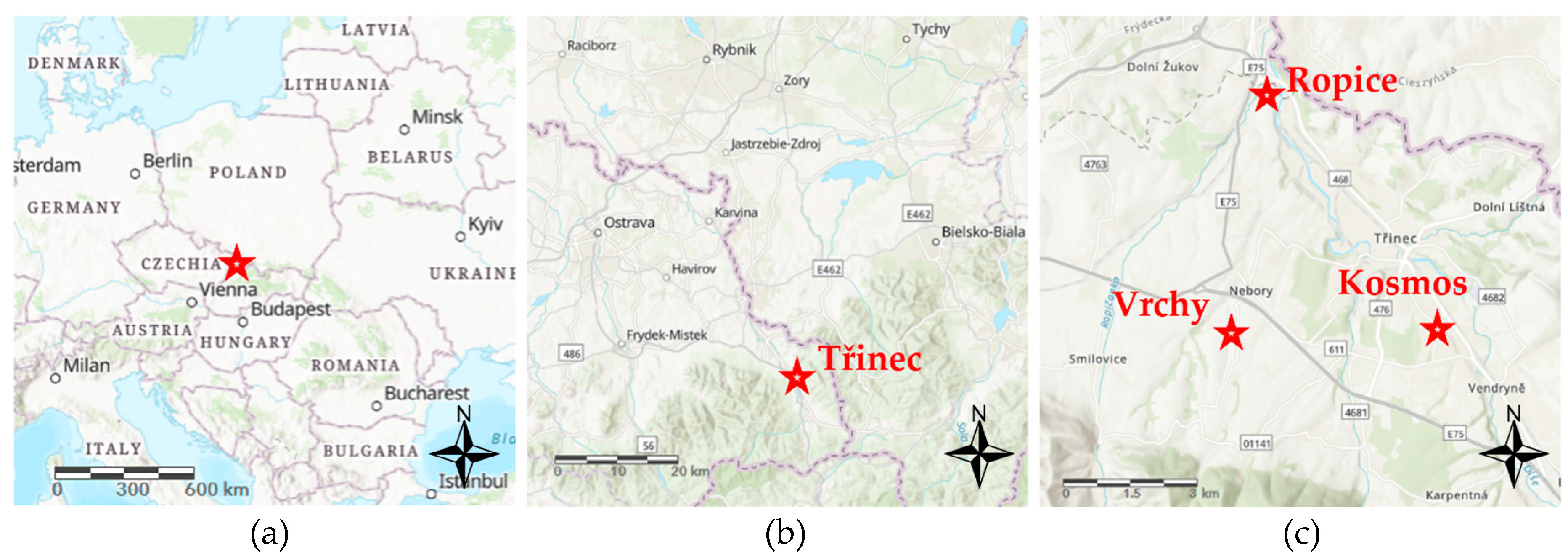
The research area is located in the eastern part of the Czech Republic, in the Moravian-Silesian Region, in the vicinity of the international border with Poland (Figure 1a,b). The area of interest includes the town of Třinec and its surroundings up to a distance of tens of kilometers. In order to identify the sources by means of PMF, dust aerosol sampling has been carried out at three sites in the town of Třinec and its surrounding areas. These were the local areas of Kosmos, Ropice, and Vrchy (Figure 1c).

The research area is affected by emissions from a number of various air pollution source types. From the Czech sources there is emission abundance, especially as far as iron metallurgy is concerned (TŘINECKÉ ŽELEZÁRNY, a.s. integrated steelworks on the north-northwestern periphery of the town of Třinec, approximately in the middle between the below-described sampling sites of Kosmos and Ropice). The other local industrial works relate mainly to the metallurgical production in Třinec and the regionally strongly developed automotive industry [7].

From the point of view of individual residential heating, the situation here is similar to the wider surrounding area in Silesia. Outside the towns, there is sparse low-floor housing development with the traditional representation of coal in the fuel mixture used for residential heating [10]. The intensity of motor vehicle traffic here does not exceed the usual values in similarly urbanized locations of the Czech Republic. It is localized towards the Třinec city center and international highway corridors towards Poland and Slovakia [11].

The average yearly concentrations of PM₁₀ and PM_2.5 in the ambient air have generally been decreasing in the direction from the heavily polluted city of Ostrava and its surroundings and the Polish part of Silesia in the north-northeast, to the relatively lightly polluted mountain area of the Beskydy in the south-southwest [12]. Apart from the Beskydy area, the PM_2.5 limit of pollution exceeds the values of 20 µg.m⁻³ which is stated as the maximum limit by a regulation that comes into force in 2020 [7] (p. 179), [12]. The increased particulate matter concentrations (PM) bear relation to benzo[a]pyrene pollution, the limit of which has been exceeded several times over in the whole of the research area [7] (pp. 171–172).

The population in the research area is concentrated especially in the Olše valley, mainly in the city of Třinec. Our initial analysis, based on the population density, size, and immission concentrations, shows that within the research area, the current air pollution inflicts the highest population health hazards in the city of Třinec and in the villages located in the Jablunkov Furrow (Vendryně, Bystřice).

2. Experiments

2.1. Sampling Sites

One of the sampling sites marked in Figure 1c is Třinec-Kosmos, which is also the location of the current site of the same name of the National Air Quality Monitoring Network of the Czech Republic. The locality represents background concentrations in the residential zones in an urban environment. In the vicinity, there are a parking, four-lane roads, and residential individual houses with individual residential heating. The main industrial air pollution source in the surrounding area is an integrated steelworks, about 2 km to the north-northeast. With regard to the vicinity of the international border with Poland (about 3.5 km to the northeast), it is possible to presume significant transborder pollution transport.

The Ropice sampling site is situated in the flat valley of the River Olše, between the cities of Třinec and Český Těšín. The air pollution here is composed of industrial activity, especially in Třinec (there is an integrated steelworks in the vicinity of about 1.5 km to the southeast, and about 700 m in the same direction there is a neighboring industrial zone). Motor vehicle traffic in the surrounding areas is represented mainly by the E75 road and its two-level junction with Road II/468 about 300 m to the northwest. There are also local fugitive emissions of PM in the surrounding area (facilities for building-demolition waste use and other kinds of loose material handling), and individual residential heating. With regard to the vicinity of the international border with Poland (about 650 m to the northeast), it is also possible to expect significant transborder pollution transport here.

The Vrchy sampling site is situated in a slightly sloping area at the foothills of the Beskydy Mountains. It represents a background country location in an open, sparsely forested landscape with a diffused settlement of individual houses (the Silesian housing development). The main sources of pollution in the surrounding area are predominantly individual residential heating with solid fuels, and agricultural activities. The surrounding transport sources are mainly the newly built E75 moderately loaded four-lane highway about 850 m away.

2.2. Sample Collection

The measured species and the campaign duration followed up the evaluation requirements by means of the PMF model. The sampling campaign was designed to use the data from three sampling sites in the Třinecko area in the PMF model. By this approach, different sources influencing the air quality in different parts of Třinecko were taken into account and a larger dataset was used, as it allowed to achieve more robust and more representative PMF results than could be provided by modeling of the individual locations. Samples collected at different sites have already been used in many other PMF source apportionment studies and, the approach has proven to increase the statistical significance of the analysis, although it assumes that the chemical profiles of the sources do not vary at the different sites [13] (pp. 134–136). The measurement at the three locations mentioned in Section 1 and Section 2.1 was divided into summer and winter sampling. The summer sampling was carried out from 5 June 2018 at 6:00 a.m. to 4 July 2018 at 6:00 p.m. The winter sampling was carried out from 14 December 2018 at 6:00 a.m. to 21 January 2019 at 6:00 p.m. All times in this article are stated in coordinated universal time (UTC). The number of samples collected and subsequently lab processed during the summer campaign was 54 (Ropice) up to 56 (Vrchy), and during the winter campaign, the number ranged from 70 (Kosmos and Vrchy) to 78 (Ropice). In the case of both the ICP-MS (mass spectrometry with inductively coupled plasma) and ED XRF (energy-dispersive X-ray spectroscopy) datasets, the time series of total size from 125 (Kosmos) to 126 (Ropice and Vrchy) samples has been used for the PMF model (sum of the summer and winter samples). The number of samples has been sufficient for reliable source apportionment based on the PMF model, as it is in accordance with its official user guide [14] (PMF is often used on speciated PM_2.5 datasets with a size above 100 samples).

Three sequence automatic samplers (Sven Leckel SEQ, Ingenieurbüro GmbH, Berlin, Germany) and one manual sampler (Sven Leckel MVS, Ingenieurbüro GmbH, Berlin, Germany) have been placed at every sampling site. The samples for PAHs and selected organic molecular tracers were collected simultaneously on 47 mm quartz fiber filters and on polyurethane foam (PUF, density 0.022 g/cm³) to collect both solid and gas–phase components of the PAHs. The same quartz fiber filters were used to collect samples for a levoglucosan analysis. The samples for other species analyses were collected on 47 mm glass fiber filters, with the exception of the analysis using the ICP-MS method, which was carried out on cellulose nitrate filters of the same diameter. At the Ropice sampling site, one Leckel SEQ automatic sequence sampler was operated for sampling on 47 mm Teflon filters for subsequent analysis using the ED XRF method.

All the dust aerosol samples were collected continuously for 12 h. For the collection of all the samples, sampling flows and collection heads were used, ensuring representative sampling of PM_2.5 fraction. The measurement of gas pollutants was carried out at the Ropice and Vrchy sites by automatic continuous analyzers placed in the mobile air quality monitoring vehicles. At all the sites, the wind speed and direction were monitored throughout the entire measurement process.

2.3. Laboratory Analyses

The lab analyses were performed in the Czech Hydrometeorological Institute, with the exception of determining the Na⁺, K⁺, Ca²⁺, and Mg²⁺ concentrations, which was done in the laboratories of the “ALS Czech Republic, s.r.o.” company (Prague, Czechia), and determining levoglucosan, which was done in the laboratories of the Institute of Chemical Process Fundamentals (ICPF) of the Czech Academy of Sciences. In all the collected aerosol samples, the same species were analyzed using the following methods to determine the ambient air concentrations:

• gravimetric analysis: PM_2.5 mass
• thermo-optical transmission: organic and elemental carbon (OC/EC)
• spectrometric analysis: ammonia (NH₄⁺)
• optical emission spectrometry with inductively coupled plasma (ICP-OES): Na⁺, K⁺, Ca²⁺, Mg²⁺
• ion chromatography with conductivity detection (IC-CD): sulfates and nitrates (SO₄²⁻, NO₃⁻)
• gas chromatography with mass detection (GC-MS):

  ○

  PAH (anthracene (A), benzo[a]anthracene (BaA), benzo[a]pyrene (BaP), benzo[b]fluoranthene (BbF), benzo[e]pyrene (BeP), benzo[ghi]perylene (BghiPRL), benzo[j]fluoranthene (BjF), benzo[k]fluoranthene (BkF), coronene (COR), chrysene (CRY), dibenz[a,h]anthracene (DBahA), phenanthrene (FEN), fluorene (Fl), fluoranthene (FLU), indeno[1,2,3-cd]pyrene (I123cdP), picene (PIC), perylene (PRL), pyrene (PYR), retene (RET)),

  ○

  hopanes (17α(H)-22,29,30-trisnorhopane, 17α(H),21β(H)-30-norhopane, 17α(H),21β(H)-hopane, 17β(H),21α(H)-hopane, 22S-17α(H),21β(H)- homohopane, 22R-17α(H),21β(H)-homohopane),

  ○

  steranes (ααα 20S-cholestane, αββ (20R)-cholestane, ααα 20R-cholestane, αββ 20R 24S-methylcholestane, αββ 20R 24R-ethylcholestane, ααα 20R 24R-ethylcholestane)

• mass spectrometry with inductively coupled plasma (ICP-MS): Li, B, Na, Mg, Al, Si, K, Ca, Ti, V, Cr, Mn, Fe, Co, Ni, Cu, Zn, Ga, Ge, As, Se, Rb, Sr, Mo, Pd, Ag, Cd, In, Sn, Sb, Te, Cs, Ba, La, Ce, Pr, Nd, Sm, Eu, Gd, Tb, Dy, Ho, Er, Tm, Yb, Lu, Hf, Ta, W, Re, Hg, Tl, Pb, Bi, Th, U
• high-performance anion-exchange chromatography with pulsed amperometric detection (IC HPAE-PAD): levoglucosan
• continuous analyzer measurement:

  ○

  UV-fluorescence (Teledyne Advanced Pollution Instrumentation T100): SO₂

  ○

  chemiluminescence (Teledyne Advanced Pollution Instrumentation T200): nitrogen oxides (NO, NO₂, NO_x)

  ○

  optoelectronic method (FIDAS 200): PM_2.5, PM₁₀

At the Ropice site, within the usability of ED XRF testing, species concentrations were also determined by means of this method in the following scale: Na, Mg, Al, Si, S, K, Ca, Ti, V, Cr, Mn, Fe, Ni, Cu, Zn, As, Se, Cd, Sb, Ba, and Pb. A parallel set of results as an alternative to the results of ICP-MS was thus acquired for subsequent receptor modeling.

3. Results

3.1. Wind Speed and Direction at the Sampling Sites

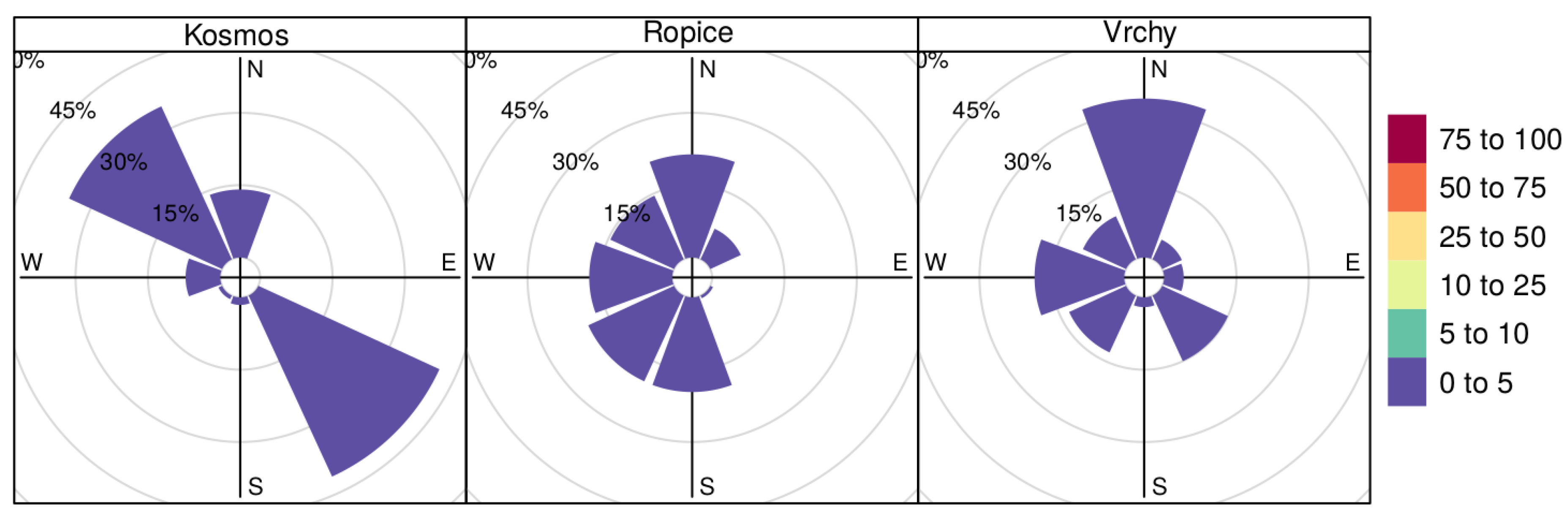
The following wind roses (Figure 2) document the situation at the sampling sites during the summer and winter sampling campaigns.

In order to interpret the modeling outputs and evaluate the predictive values of the assessment, the wind direction and speed were compared and measured during the sampling campaigns, with the average at the Kosmos site, which is also a site of the National Air Quality Monitoring Network of the Czech Republic, for the years 2009–2018. The prevailing wind direction corresponds to its long-term average. The average wind speed was generally higher (about 1.6 m.s⁻¹ at the time of sampling) as opposed to its long-term average (about 1.3 m.s⁻¹).

3.2. Analysis of the Measured Concentrations

The summary

Table 1. Species quantified in this study (summary of all 3 sampling sites). Std. Dev.:Standard deviation; BDL: Below detection limit; N/A: no data available.

	SUMMER				WINTER
Species	Mean (ng.m−3)	Std. Dev. (ng.m−3)	Percent Missing	Percent BDL	Mean (ng.m−3)	Std. Dev. (ng.m−3)	Percent Missing	Percent BDL
PM2.5	1.3 × 104	6.0 × 103	0%	0%	2.8 × 104	3.4 × 104	0%	0%
Li (ICP)	1.3 × 10−1	8.7 × 10−2	2%	88%	1.7 × 10−1	2.2 × 10−1	7%	2%
B (ICP)	5.0 × 100	3.2 × 100	2%	24%	5.2 × 100	6.6 × 100	7%	26%
Na (ICP)	8.6 × 101	7.3 × 101	2%	36%	1.1 × 102	1.1 × 102	7%	0%
Mg (ICP)	2.9 × 101	1.8 × 101	2%	4%	2.0 × 101	7.0 × 101	7%	10%
Al (ICP)	5.6 × 101	4.6 × 101	2%	10%	3.0 × 101	2.0 × 102	7%	4%
Si (ICP)	1.0 × 102	1.5 × 102	2%	42%	1.2 × 102	1.9 × 102	7%	48%
K (ICP)	1.1 × 102	1.3 × 102	2%	25%	2.8 × 102	9.4 × 102	7%	1%
Ca (ICP)	9.8 × 101	7.2 × 101	2%	9%	2.9 × 101	5.4 × 101	7%	16%
Ti (ICP)	1.3 × 100	8.8 × 10−1	2%	6%	6.8 × 10−1	1.3 × 100	7%	3%
V (ICP)	3.5 × 10−1	2.1 × 10−1	2%	5%	1.5 × 10−1	1.8 × 10−1	7%	0%
Cr (ICP)	3.6 × 100	2.3 × 100	2%	10%	1.1 × 100	2.0 × 100	7%	26%
Mn (ICP)	8.6 × 100	1.3 × 101	2%	5%	6.4 × 100	1.4 × 101	7%	0%
Fe (ICP)	2.4 × 102	3.8 × 102	2%	5%	1.7 × 102	3.7 × 102	7%	3%
Co (ICP)	4.3 × 10−2	3.5 × 10−2	2%	12%	5.2 × 10−2	6.7 × 10−2	7%	0%
Ni (ICP)	1.3 × 100	2.1 × 100	2%	36%	8.1 × 10−1	1.6 × 100	7%	25%
Cu (ICP)	4.6 × 100	3.4 × 100	2%	5%	4.6 × 100	1.6 × 101	7%	15%
Zn (ICP)	3.6 × 101	3.7 × 101	2%	5%	3.4 × 101	8.0 × 101	7%	0%
Ga (ICP)	1.6 × 10−1	1.3 × 10−1	2%	3%	3.5 × 10−1	7.6 × 10−1	7%	0%
Ge (ICP)	6.9 × 10−2	1.1 × 10−1	2%	6%	1.1 × 10−1	1.4 × 10−1	7%	0%
As (ICP)	7.7 × 10−1	7.0 × 10−1	2%	4%	1.3 × 100	1.3 × 100	7%	0%
Se (ICP)	6.6 × 10−1	4.2 × 10−1	2%	18%	4.5 × 10−1	5.5 × 10−1	7%	6%
Rb (ICP)	4.1 × 10−1	5.8 × 10−1	2%	5%	7.2 × 10−1	9.3 × 10−1	7%	0%
Sr (ICP)	5.5 × 10−1	3.7 × 10−1	2%	6%	1.5 × 100	1.2 × 101	7%	6%
Mo (ICP)	6.8 × 10−1	1.6 × 100	2%	3%	4.8 × 10−1	1.1 × 100	7%	0%
Pd (ICP)	1.2 × 10−3	6.3 × 10−4	2%	82%	1.8 × 10−3	7.8 × 10−3	7%	29%
Ag (ICP)	3.6 × 10−2	3.4 × 10−2	2%	7%	3.1 × 10−2	3.5 × 10−2	7%	6%
Cd (ICP)	2.1 × 10−1	2.0 × 10−1	2%	1%	2.6 × 10−1	3.1 × 10−1	7%	3%
In (ICP)	7.8 × 10−3	7.3 × 10−3	2%	32%	9.0 × 10−3	1.2 × 10−2	7%	1%
Sn (ICP)	1.3 × 100	1.1 × 100	2%	3%	1.0 × 100	1.1 × 100	7%	1%
Sb (ICP)	8.7 × 10−1	6.6 × 10−1	2%	3%	5.8 × 10−1	6.6 × 10−1	7%	0%
Te (ICP)	8.2 × 10−3	9.4 × 10−3	2%	14%	1.1 × 10−2	2.1 × 10−2	7%	7%
Cs (ICP)	7.3 × 10−2	1.5 × 10−1	2%	6%	1.1 × 10−1	2.1 × 10−1	7%	0%
Ba (ICP)	1.8 × 100	1.1 × 100	2%	5%	4.1 × 100	3.1 × 101	7%	18%
La (ICP)	4.0 × 10−2	3.0 × 10−2	2%	12%	1.2 × 10−2	1.8 × 10−2	7%	11%
Ce (ICP)	7.7 × 10−2	5.7 × 10−2	2%	10%	2.2 × 10−2	3.7 × 10−2	7%	8%
Pr (ICP)	9.4 × 10−3	8.3 × 10−3	2%	19%	2.0 × 10−3	2.2 × 10−3	7%	21%
Nd (ICP)	3.4 × 10−2	3.0 × 10−2	2%	9%	8.3 × 10−3	8.9 × 10−3	7%	14%
Sm (ICP)	6.8 × 10−3	5.9 × 10−3	2%	26%	2.0 × 10−3	2.2 × 10−3	7%	16%
Eu (ICP)	2.0 × 10−3	1.3 × 10−3	2%	41%	2.5 × 10−3	1.3 × 10−2	7%	28%
Gd (ICP)	7.3 × 10−3	6.2 × 10−3	2%	19%	2.7 × 10−3	2.6 × 10−3	7%	12%
Tb (ICP)	1.1 × 10−3	7.4 × 10−4	2%	24%	7.6 × 10−4	2.9 × 10−4	61%	4%
Dy (ICP)	5.0 × 10−3	4.0 × 10−3	2%	20%	1.5 × 10−3	1.7 × 10−3	7%	23%
Ho (ICP)	1.1 × 10−3	7.4 × 10−4	2%	23%	8.1 × 10−4	3.0 × 10−4	57%	3%
Er (ICP)	3.0 × 10−3	2.2 × 10−3	2%	31%	1.1 × 10−3	7.7 × 10−4	7%	68%
Tm (ICP)	6.4 × 10−4	3.6 × 10−4	2%	54%	6.2 × 10−4	1.7 × 10−4	80%	5%
Yb (ICP)	2.8 × 10−3	2.1 × 10−3	2%	35%	1.0 × 10−3	1.0 × 10−3	7%	30%
Lu (ICP)	5.5 × 10−4	3.1 × 10−4	2%	67%	5.8 × 10−4	1.9 × 10−4	88%	4%
Hf (ICP)	6.0 × 10−3	4.5 × 10−3	2%	14%	2.7 × 10−3	4.4 × 10−3	7%	12%
Ta (ICP)	1.4 × 10−1	2.7 × 10−1	2%	64%	6.1 × 10−2	1.2 × 10−1	7%	61%
W (ICP)	6.4 × 10−2	7.5 × 10−2	2%	6%	8.5 × 10−2	9.4 × 10−2	7%	3%
Re (ICP)	2.3 × 10−3	5.2 × 10−3	2%	30%	1.6 × 10−3	1.6 × 10−3	26%	0%
Hg (ICP)	1.0 × 10−1	1.5 × 10−1	2%	94%	1.7 × 10−1	2.6 × 10−1	7%	27%
Tl (ICP)	6.0 × 10−2	5.2 × 10−2	2%	11%	1.3 × 10−1	2.0 × 10−1	7%	0%
Pb (ICP)	8.5 × 100	7.8 × 100	2%	1%	1.1 × 101	1.4 × 101	7%	0%
Bi (ICP)	2.4 × 10−1	3.0 × 10−1	2%	2%	7.3 × 10−1	5.2 × 100	7%	3%
Th (ICP)	7.4 × 10−3	5.9 × 10−3	2%	16%	1.5 × 10−3	1.7 × 10−3	7%	27%
U (ICP)	7.1 × 10−3	6.8 × 10−3	2%	29%	7.9 × 10−3	1.3 × 10−2	7%	55%
OC	4.3 × 103	1.7 × 103	0%	0%	1.9 × 103	2.3 × 103	7%	0%
EC	5.2 × 102	3.1 × 102	0%	0%	1.1 × 104	1.3 × 104	7%	0%
sulphates	2.7 × 103	1.1 × 103	0%	0%	3.2 × 103	2.7 × 103	7%	0%
nitrates	1.3 × 103	7.1 × 102	0%	0%	2.2 × 103	2.0 × 103	7%	0%
ammonium ion	5.0 × 102	3.9 × 102	0%	0%	1.2 × 103	1.4 × 103	7%	0%
Fluorene	7.5 × 100	5.0 × 100	5%	1%	2.4 × 101	1.9 × 101	11%	0%
Phenanthrene	1.3 × 101	6.7 × 100	5%	0%	4.8 × 101	3.1 × 101	11%	0%
Anthracene	3.8 × 10−1	3.1 × 10−1	5%	0%	5.3 × 100	5.5 × 100	11%	0%
Fluoranthene	3.1 × 100	1.5 × 100	5%	0%	1.9 × 101	1.5 × 101	11%	0%
Pyrene	1.5 × 100	7.7 × 10−1	5%	0%	1.3 × 101	1.2 × 101	11%	0%
Benz[a]anthracene	3.0 × 10−1	2.5 × 10−1	5%	1%	6.8 × 100	7.9 × 100	11%	0%
Chrysene	3.8 × 10−1	2.5 × 10−1	5%	0%	5.0 × 100	5.4 × 100	11%	0%
Benzo[b]fluoranthene	4.6 × 10−1	3.5 × 10−1	5%	0%	4.0 × 100	3.8 × 100	11%	0%
Benzo[k]fluoranthene	2.2 × 10−1	1.7 × 10−1	5%	2%	2.1 × 100	2.0 × 100	11%	0%
Benzo[j]fluoranthene	2.4 × 10−1	1.8 × 10−1	5%	1%	1.9 × 100	1.9 × 100	11%	0%
Benzo[a]pyrene	3.2 × 10−1	2.3 × 10−1	5%	1%	3.9 × 100	4.3 × 100	11%	0%
Indeno[1,2,3-cd]pyrene	2.9 × 10−1	2.8 × 10−1	5%	6%	4.4 × 100	4.5 × 100	11%	0%
Dibenz[a,h]anthracene	1.5 × 10−1	1.4 × 10−1	5%	6%	9.9 × 10−1	1.0 × 100	11%	0%
Benzo[g,h,i]perylene	2.8 × 10−1	2.2 × 10−1	5%	2%	2.9 × 100	3.0 × 100	11%	0%
Coronene	9.2 × 10−2	6.0 × 10−2	5%	11%	8.5 × 10−1	9.1 × 10−1	11%	0%
Perylene	6.9 × 10−2	5.1 × 10−2	5%	26%	5.9 × 10−1	6.4 × 10−1	11%	2%
Retene	2.1 × 10−1	1.3 × 10−1	5%	1%	2.5 × 100	2.9 × 100	11%	0%
Picene	8.4 × 10−2	4.7 × 10−2	5%	11%	8.3 × 10−1	1.0 × 100	11%	0%
Benzo[e]pyrene	2.9 × 10−1	2.3 × 10−1	5%	1%	2.0 × 100	2.0 × 100	11%	0%
Na+	4.2 × 103	1.4 × 103	0%	0%	2.5 × 103	6.4 × 102	7%	0%
K+	1.7 × 102	1.1 × 102	0%	2%	3.3 × 102	1.4 × 103	7%	0%
Ca2+	5.1 × 103	1.6 × 103	0%	0%	3.4 × 103	9.8 × 102	7%	0%
Mg2+	6.2 × 102	3.1 × 102	0%	0%	3.1 × 102	1.4 × 102	7%	0%
levoglucosan	7.8 × 101	7.1 × 101	0%	1%	5.8 × 102	5.7 × 102	7%	0%
SO2	7.1 × 103	3.9 × 103	67%	0%	8.8 × 103	8.2 × 103	70%	0%
NO	1.2 × 103	1.0 × 103	33%	0%	2.9 × 103	5.1 × 103	36%	0%
NO2	1.1 × 104	6.5 × 103	33%	0%	1.4 × 104	1.1 × 104	36%	0%
CO	2.1 × 105	2.6 × 104	95%	0%	4.8 × 105	4.8 × 105	36%	0%
O3	N/A	N/A	100%	0%	3.9 × 104	1.6 × 104	9%	0%
ααα 20R-Cholestane	9.9 × 10−2	8.4 × 10−2	7%	64%	9.5 × 10−2	3.1 × 10−2	16%	82%
ααα 20R 24R-Ethylcholestane	N/A	N/A	100%	0%	2.3 × 10−1	2.4 × 10−1	11%	49%
17α(H)-22,29,30-Trisnorhopane	9.6 × 10−2	5.4 × 10−2	7%	57%	5.7 × 10−1	6.7 × 10−1	10%	2%
17α(H),21β(H)-30-Norhopane	2.0 × 10−1	1.1 × 10−1	7%	54%	7.9 × 10−1	7.7 × 10−1	10%	0%
17α(H),21β(H)-Hopane	2.8 × 10−1	1.8 × 10−1	7%	77%	9.0 × 10−1	8.9 × 10−1	10%	0%
17β(H),21α(H)-Hopane	7.1 × 10−2	3.0 × 10−2	7%	81%	4.1 × 10−1	4.5 × 10−1	10%	3%
17α(H),21β(H)-22S-Homohopane	2.1 × 10−1	1.2 × 10−1	7%	85%	3.7 × 10−1	4.7 × 10−1	10%	2%
17α(H),21β(H)-22R-Homohopane	1.1 × 10−1	7.1 × 10−2	7%	73%	7.0 × 10−1	8.3 × 10−1	10%	0%

lists the mean species concentrations, standard deviations, and percentages of missing and below-detection-limit observations. In the case of metals, only the ICP-MS results are listed in the table, as they are available at all three sampling sites, as opposed to the ED XRF results, which were measured at the Ropice site only.

The measured data show significantly higher concentrations and time variations of heavy PAHs, levoglucosan, retene, picene, and elemental carbon during the winter sampling campaign (about or more than one order of magnitude). On the other hand, most of the typical crustal species, like Mg, Al, Ca, T, and lanthanoides, plus organic carbon, show higher concentrations and variations in the summer. The highest PM_2.5 concentrations were detected at Ropice, somewhat lower concentrations at the Kosmos site and the significantly lowest concentrations at the Vrchy site. In the time series of some metals and hopanes, a sizable percentage of values occurred below the detection limit of the laboratory methods. These cases tended to occur more often in the summer period. The laboratory method sensitivity to detect the concentrations of other analytes was sufficient to reliably quantify its concentrations.

Table 2. Species concentrations at the Ropice site measured by ICP-MS and ED XRF during the summer sampling period. Std. Dev.: Standard deviation; BDL: Below detection limit.

	ICP-MS				ED XRF
Species	Mean (ng.m−3)	Std. Dev. (ng.m−3)	Percent Missing	Percent BDL	Mean (ng.m−3)	Std. Dev. (ng.m−3)	Percent Missing	Percent BDL
Na	8.5 × 101	7.4 × 101	5%	39%	5.3 × 101	3.8 × 101	0%	10%
Mg	3.1 × 101	2.3 × 101	5%	2%	1.0 × 102	4.8 × 101	0%	0%
K	1.2 × 102	1.5 × 102	5%	39%	1.1 × 102	8.8 × 101	0%	19%
Ca	1.1 × 102	9.0 × 101	5%	4%	8.5 × 101	7.4 × 101	0%	0%
Ti	1.4 × 100	7.1 × 10−1	5%	0%	3.8 × 100	3.0 × 100	0%	0%
V	3.8 × 10−1	2.2 × 10−1	5%	0%	2.4 × 10−1	1.2 × 10−1	0%	0%
Cr	4.3 × 100	3.5 × 100	5%	9%	3.9 × 100	1.4 × 100	0%	0%
Mn	1.4 × 101	2.2 × 101	5%	0%	1.4 × 101	2.1 × 101	0%	0%
Fe	3.9 × 102	6.3 × 102	5%	0%	3.6 × 102	5.3 × 102	0%	0%
Ni	2.1 × 100	3.1 × 100	5%	27%	1.1 × 100	2.6 × 100	0%	0%
Cu	6.0 × 100	4.8 × 100	5%	4%	5.0 × 100	4.4 × 100	0%	0%
Zn	5.1 × 101	4.7 × 101	5%	0%	5.8 × 101	5.1 × 101	0%	2%
As	1.0 × 100	9.7 × 10−1	5%	0%	4.1 × 10−1	3.9 × 10−1	0%	0%
Se	8.5 × 10−1	4.6 × 10−1	5%	11%	1.1 × 100	4.9 × 10−1	0%	0%
Sb	1.1 × 100	7.8 × 10−1	5%	0%	-2.3 × 101	1.2 × 101	0%	0%
Ba	1.8 × 100	8.9 × 10−1	5%	2%	1.6 × 100	9.3 × 10−1	0%	0%
Pb	1.1 × 101	1.1 × 101	5%	0%	1.2 × 101	1.1 × 101	0%	2%

and

Table 3. Species concentrations at the Ropice site measured by ICP-MS and ED XRF during the winter sampling period. Std. Dev.: Standard deviation; BDL: Below detection limit.

	ICP-MS				ED XRF
Species	Mean (ng.m−3)	Std. Dev. (ng.m−3)	Percent Missing	Percent BDL	Mean (ng.m−3)	Std. Dev. (ng.m−3)	Percent Missing	Percent BDL
Na	1.4 × 102	1.4 × 102	0%	0%	7.2 × 101	5.7 × 101	0%	3%
Mg	2.5 × 101	6.2 × 101	0%	15%	8.7 × 101	1.1 × 102	0%	3%
K	3.0 × 102	4.1 × 102	0%	0%	4.8 × 102	8.2 × 102	0%	1%
Ca	5.1 × 101	8.2 × 101	0%	6%	6.0 × 101	1.3 × 102	0%	0%
Ti	7.6 × 10−1	9.6 × 10−1	0%	1%	2.1 × 100	2.1 × 100	0%	0%
V	2.0 × 10−1	1.9 × 10−1	0%	0%	4.5 × 10−1	3.9 × 10−1	0%	0%
Cr	2.1 × 100	2.8 × 100	0%	15%	4.0 × 100	2.0 × 100	0%	1%
Mn	1.3 × 101	2.1 × 101	0%	0%	1.7 × 101	2.7 × 101	0%	0%
Fe	3.6 × 102	5.6 × 102	0%	4%	4.8 × 102	7.7 × 102	0%	4%
Ni	1.1 × 100	2.2 × 100	0%	29%	1.5 × 100	4.8 × 100	0%	0%
Cu	6.2 × 100	1.3 × 101	0%	14%	9.8 × 100	2.3 × 101	0%	0%
Zn	5.7 × 101	1.3 × 102	0%	0%	9.0 × 101	1.7 × 102	0%	3%
As	1.8 × 100	1.8 × 100	0%	0%	9.8 × 10−1	8.8 × 10−1	0%	0%
Se	6.6 × 10−1	8.1 × 10−1	0%	6%	1.6 × 100	1.5 × 100	0%	0%
Sb	7.9 × 10−1	9.2 × 10−1	0%	0%	3.5 × 10−1	8.0 × 10−1	0%	0%
Ba	4.0 × 100	2.4 × 101	0%	5%	3.7 × 100	2.1 × 101	0%	0%
Pb	1.8 × 101	1.9 × 101	0%	0%	2.4 × 101	2.2 × 101	0%	1%

list the mean species concentrations, standard deviations, and percentages of missing and below-detection-limit observations at the Ropice sampling site provided by ICP-MS and ED XRF methods in the summer and winter samplings, respectively.

Both ICP-MS and ED XRF show a similar seasonal variation of concentrations, as shown in Table 1 (visibly higher crustal species concentrations in summer, and potassium and heavy metals strongly related to biomass and coal combustion in winter). Due to the low reliability of measuring Al, Si, and Cd by the ED XRF, which was found during previous internal measuring tests of this method, this species has been excluded from the comparison of methods in Table 2; Table 3.

The majority of the species showed nearly lognormal distribution. Only in the case of ozone did the dataset come anywhere near normal distribution. Part of the analytes showed bimodal distribution denotative of the influence of at least two different pollution sources. As a significantly larger number of datasets thus affected was detected at the Kosmos and Vrchy sites, it is probably the result of pollution transport from more remote areas during specific meteorological conditions, while at Ropice, pollution from neighboring sources has a greater impact. At the Kosmos and Ropice sampling sites, the statistical distribution of some species concentrations was more deformed in the area of high values. It is likely to be connected with the occurrence of intensive concentration peaks at these more polluted locations (the result of meteorological situations that rarely occur, but bring high pollution concentrations).

On average, the majority of the measured species has had higher concentrations in the winter period and at night, which goes hand in hand with the series of PM_2.5 concentration. Significantly higher winter concentrations were detected mainly regarding species, the emissions of which are associated with residential heating by solid fuels. They are As, K, K⁺, levoglucosan, retene, picene, EC, and PAH. Apart from these, concentrations several times higher were also detected in the cold half of the year, as opposed to the summer campaign, in the case of nitrogen oxides and nitrates.

In order to evaluate the basic relations among the measured species, correlation matrices have been elaborated, onto which a cluster analysis has been applied by means of the R statistical software. The result of the cluster analysis preliminarily indicated five factors influencing the variability of the measured species concentrations.

3.3. Positive Matrix Factorization (PMF) Modeling

PMF model 5.0 was used in accordance with the U.S. EPA Positive Matrix Factorization (PMF), Fundamentals and User Guide [14]. Based on parallel analyses from Ropice using the ICP-MS and ED XRF methods, an individual PMF model was elaborated for this location for each of the datasets to allow comparison of the PMF results. The results of the other laboratory analyses used in both models (see Section 2.3) were the same. Using the signal/noise ratio, the species were split into the categories of STRONG, WEAK, and BAD. 40 STRONG species were used in the case of the dataset, including the data from ICP-MS, and in the case of the ED XRF dataset, they were 33.

It was necessary to exclude a night sample from 31 December 2018 to 1 January 2019 from the time data series and the following day for the air polluted by a wide spectrum of analytes (especially Ba, Pd, Mg, Al, S, Ti, and Cu) caused by New Year’s Eve celebrations. With regard to the fact that the source of this extreme concentration peak was an isolated instance, its influence is unassessable by means of PMF. An isolated value of Zn in the sample from 21 December 2018 (6:00 a.m–6:00 p.m. UTC), which is about one order of magnitude higher than the average concentration for the rest of the measured period, was also excluded. The missing values were replaced by a median with uncertainty set at quadruple the median value. The values below the detection limit were assigned one-half of the detection limit and their uncertainty, at 5/6 of the detection limit.

Special care for gas species which do not contribute to the total PM_2.5 mass was carried out due to the risk of their possible negative effect on the model solution, e.g., creating redundant unreal factors. Many model runs with different parameters and various gas species have been carried out to test if their use leads to disturbing or complicating model solutions or if they support reasonable interpretation. During the modeling, good usability of gas species was discovered. They have acted not as the main strong markers of specific air pollution sources, but have provided useful supplementary information for profile interpretation. The NO/NO₂ ratio was used successfully when considering the effect of local/distant sources, or of fresh/altered pollution, as complementary information to nitrogen ion concentrations. In a similar way, the SO₂/sulfate ratio was kept in mind when significant effects of local sources were interpreted (e.g., steelworks and local residential heating clusters). For the mentioned reasons, NO, NO₂, and SO₂ have been incorporated in the PMF modeling dataset. Due to technical issues, ozone was measured in the winter part of the sampling campaign only. Because of this fact and the complex chemical reactivity of ozone, its role may be confusing rather than beneficial during interpretation of the model. Ozone has thus been excluded from the PMF model of Ropice. Despite the mentioned arguments, during the comprehensive modeling of all three locations ozone has been used with caution. After obtaining a rough stable model solution, ozone has been classified as WEAK and included in the PMF species. The aim of such a controvesal use of ozone has been to test the source profiles in which it tends to be present and to verify if its presence in the profiles is in agreement with the expectation. Using ozone in the comprehensive PMF dataset has been one of the complementary methods to evaluate whether the model corresponds to the real atmospheric relations. Neither the identified factors nor their contributions have been negatively affected by declaring ozone as a WEAK variable.

Using the ICP-MS and ED XRF data, the stable model solution (normal distribution and acceptable residue size in line with the PMF user guide [14], mutual independence of the identified factors, ratio Q/Q_exp, etc.) was established with 5 factors. For the final PMF solution for the Ropice location, 50 model runs have been done using both the ED XRF and ICP-MS datasets. The same number of model runs has been executed within the comprehensive model of all three sampling locations. Based on the bootstrap analysis, the ED XRF and ICP-MS model solution rotations were used with the values of Fpeak = 0.5 and 1.0, respectively. The coefficient of determination of the predicted and measured concentrations of PM_2.5 in the case of the ED XRF and ICP-MS datasets reached the values of R² = 0.91 and 0.93, respectively. The Ropice site model was elaborated with 20% extra modeling uncertainty for both the ICP-MS and ED XRF datasets.

Due to the known limitations of ED XRF (see the discussion in the Section 4.2), ICP-MS has been considered to be the main method for the source apportionment whereas ED XRF was the suplementary method for testing its ablity in PMF. In order to elaborate a comprehensive PMF model including all three sampling sites (Kosmos, Ropice, Vrchy) only the ICP-MS method element analysis results were used, as it has a wider species composition and lower uncertainty than ED XRF.

For the PMF model, 31 analytes were classified as STRONG. This comprehensive evaluation was elaborated with an 18% extra modeling uncertainty. In other parameters, the modeling methodology was identical to the model of the Ropice site.

3.4. Identified Factors and Their Contributions to PM_2.5 Concentrations Using the All-sites Model

Within the comprehensive model solution based on the ICP-MS dataset and including all 3 sampling sites, the same factors as those within the PMF model of the Ropice site have been identified. The only difference is the “residential heating” factor differentiation into two independent factors according to the kind of fuel. The chemical composition and factor time series are evident from the graphs in Appendix A and Appendix B, respectively.

Residential heating type 1: Dominant representation of polycyclic aromatic hydrocarbons (PAH), elemental carbon (EC), with an increased percentage of levoglucosan and some heavy metals (arsenic, selenium), hopanes, and nitrogen oxides. The daily variation of factor contributions fluctuates a great deal, with its maxima at night. The day/night difference in winter with stable heating operation is in no way as significant as in the summer, when there is only extra heating and hot supply water heating in the evening and the night hours.

Residential heating type 2: These are probably the same sources as in the case of the “local residential heating type 1” factor, but using other fuels or illegal waste combustion. The chemical profile is similar to the case of the “local residential heating type 1” factor, but with a higher representation of a wide spectrum of metals (antimony, cadmium, silver, tin, zinc, lead). The time series fluctuated significantly in the evaluated period, especially in the summer. In the summer as opposed to the winter period, a significantly higher contribution of this factor to the overall PM_2.5 mass was detected.

Regional aerosol: A characteristic feature of this factor is the high representation of nitrogen ions (NH₄⁺, NO₃⁻) combined with sulfates or/and sulfur, metals (vanadium, selenium, tin, indium, arsenic) and hopanes and an increased contribution of organic carbon. In the signature of the regional aerosol, the influence of coal combustion in individual residential heating sources is evident (sulfur, vanadium, selenium, arsenic), and also, most likely, of motor vehicle traffic (nitrogen ions and nitrogen oxides). Its chemical composition and the factor time series imply that, apart from the primary suspended particles (emitted directly from the pollution sources), it also includes secondary aerosol. The factor contribution time series is marked by somewhat lower variability in the course of the sampling campaign as opposed to the locally occurring residential heating. In the winter period, several sequences of consecutive days of increased values were detected when the concentrations, as opposed to local source fingerprints, did not decrease to low values as fast as in the case of “Residential heating” factors, which bears evidence of pollution transported from longer distances. During some high pollution episodes in the winter, delayed entrance of this factor after the residential heating factor was noticed, which probably corresponded to the gradual rise of a secondary aerosol in the region during deteriorated dispersion conditions.

Crustal: This is, above all, resuspended dust from the Earth’s surface lifted by the wind and road traffic. In its chemical profile, an increased percentage of species abundant in the Earth’s crust is thus prominent (aluminum, barium, strontium, titanium). In comparison with other factor profiles, these elements are accompanied by increased concentrations of ozone, which corresponds to the relatively high contribution of this factor in the period with intense sunshine. The high percentage of organic carbon and, meanwhile, the low percentage of elemental carbon, testify to the presence of an important biogenic component, probably especially pollen and biogenic particles in the summer period of the sampling campaign. This issue is further discussed in Section 4. The factor is typical for its significant daily variation with the maxima during the day. In a yearly course, higher factor contribution in the warm part of the year was discovered; in the course of the winter sampling campaign, the contribution of this factor was close to zero.

Long-range transport: The chemical profile contains particles of which the composition is mostly sea salt (ions Na⁺, Mg²⁺, Ca²⁺), sulfates, nitrates, and ozone with the representation of hopanes. Less significantly, nitrogen oxides demonstrate in its signature. In its chemical profile, a small percentage of coal combustion emissions also demonstrates (arsenic and selenium), probably originating from large industrial energy sources. It is apparent that it is a mixture of sea aerosol with a secondary aerosol that is developed from primary anthropogenic emissions in the course of its long transport time. The factor demonstrates itself by a time series with unremarkable day/night variation and by the relatively lowest difference of the concentration’s contribution out of all the identified factors between the summer and winter parts of the campaign.

Iron and steelworks: A factor composed of dominant percentage of iron and manganese accompanied by molybdenum and, relatively less significantly, by a wide spectrum of other metals (lead, indium, thallium, silver, cobalt, zinc, arsenic, selenium, and strontium), which corresponds to the complex production of iron, steel, and relevant productions in the large industrial premises surrounding the TŘINECKÉ ŽELEZÁRNY, a.s. plant. The factor time series is extremely variable, depending on the wind direction (very high contribution to PM_2.5 concentration when the emission plume heads towards the sampling site from the metallurgical plant, as opposed to the almost zero influence in other cases). The average size of the factor contribution in the warm and cold parts of the sampling campaign was similar.

The apportioned percentages and PM_2.5 concentrations of the main air pollution sources are illustrated in the following graph (Figure 3).

3.5. The Conformity of the Identified Factors and Their Contributions to PM_2.5 Concentrations Using ICP-MS and ED XRF Datasets at the Ropice Site

The identified factors at the Ropice site were identical when using both compared analytical methods (ICP-MS and ED XRF): local residential heating, regional aerosol, long-range transport, iron and steelworks, and crustal. Figure 4 and Figure 5 show the chemical profiles of the factors identified by PMF using the ICP-MS and ED XRF datasets.

The PMF model with the ICP-MS and ED XRF datasets is based on partly different species composition, and, therefore, direct comparison of the model results is impossible. As shown in Figure 4 and Figure 5, with ICP-MS and ED XRF datasets, the same characteristic diagnostic species groups are present in the chemical profiles, which have led to the same identified factors. The final solution is easily interpretable: “Residential heating” stands out by PAHs, elemental carbon, levoglucosan percentage, and relatively high 17α(H),21β(H)-22R-Homohopane / 17α(H),21β(H)-22S-Homohopane ratio (due to the frequent burning of low-quality coal). “Regional aerosol” is rich in nitrogen ions and sulfates (in the case of the ED XRF dataset, also in sulfur) as a manifestation of chemical-transformed road traffic and coal-burning emissions. The “crustal” factor contains significant percentages of Mg, Al, Ca, and Ba (ICP-MS dataset), and Ca, Ti, and Ba (ED XRF dataset), respectively. Long-range transport is typical in its high sea-salt percentage with sulfates, nitrates, and a relatively low 17α(H),21β(H)-22R-Homohopane / 17α(H),21β(H)-22S-Homohopane ratio. The iron and steelworks chemical profile is characteristic for its dominant percentage of Fe, Mn, and a wide spectrum of heavy metals in combination with nitrogen oxides.

Overall, the PMF factor profiles based on both the ICP-MS and ED XRF datasets are similar and contain the same diagnostic species (further discussion on the specifics of chemical profiles is a part of Section 4). The identified factors at the Ropice site are the same as the comprehensive all-sites PMF model factors, which were explained in more detail in Section 3.4.

3.6. Pollution Source Areas

Based on the time series of the factor contributions to PM_2.5 concentrations and hourly values of the wind direction and speed at individual sampling sites, time-weighted concentration roses and CPF (Conditional Probability Function) graphs have been elaborated, based on which it is possible to determine the directions of the main pollution origins. The time-weighted concentration roses include all the model quantified values; the CPF has been visualized for the contribution values exceeding the 90th percentile. The time-weighted concentration roses of the identified factor contributions form Appendix C. The CPF graphs proved to have little illustrative value and do not contain enough information; that is why they are not part of the article. The determination of the pollution source areas was limited by the amount of data available (about 130 values for each location). Thus, for a more precise source localization, it was inefficient to apply some methods that are more demanding as far as a statistical file size is concerned, e.g., PSCF (potential source contribution function).

Local residential heating type 1: At the Kosmos site, the factor acts especially from the direction of the densely populated Jablunkov Furrow (probably the influence of Vendryně, Bystřice, and other villages) and from the north-northwest (probably the influence of the periphery of Třinec). At Ropice the main part of this pollution type is transported from two prevailing directions, north (Olše valley) and south. In both cases, with regard to the high average contributions from these directions, the factor is the influence of the local residential development nearby. The Vrchy site is significantly different in this respect. The factor here acts mainly from the north, and, with respect to the occurrence of both high and low factor contributions, it is probably a combination of the local sources from the Vrchy part as well as the influence from more remote areas, e.g., the Nebory development part.

Local residential heating type 2: At the Kosmos site, the most intense concentration peaks of this factor occurred when the wind originated from the northwest (influence of peripheral parts of the city of Třinec in the Olše valley). A significant contribution here occurs both in the warm and cold halves of the year. In winter, however, pollution transport prevails from the southeast. At the Ropice and Vrchy sites, the main source areas are identical to the local residential heating type 1 factor.

Regional aerosol: At the Kosmos and Ropice sites, the winter contribution was approximately double as opposed to the summer contribution, and the main pollution origin directions are analogical, as in the case of the residential heating type 1 and 2 factors (from Jablunkov Furrow and sites situated at lower locations in the Olše valley. At Ropice, however, this occurred most significantly from the south). At the Vrchy site, on the contrary, from the point of view of both the maxima and the average contribution values, northwest wind directions dominate, which shows pollution transport not only from the neighboring areas of the city of Třinec, but also from the city of Ostrava and its surroundings or villages situated in this direction.

Crustal: At the Kosmos site, factor contributions prevail from the southeast and northwest, and at the Ropice site, from the north and especially the south. At the Vrchy site, although the contribution peaks are connected with a southwest wind direction, probably from the nearby local source (field work), meteorological situations with north and southeast wind directions had a decisive influence on the average factor contribution here.

Long-range transport: The main average contribution of long-range transport comes from the north-northwest. The less significant part of the long-range pollution transport was captured at the Kosmos and Vrchy sites in periods with a southeastern wind, thus from the corridor of Jablunkov Furrow. At Ropice, it came from the southern direction.

Iron and steelworks: At the Kosmos site, which is situated windward of the integrated metallurgical plant, the high factor contributions occurred during the northwest current. At Ropice, which is situated leeward of the metallurgical sources, there were dominant contributions from the south and southeast. At the background countryside site of Vrchy, the quantified contributions of this factor reached very low values; the determination of the source direction is thus unreliable here. For guidance, the origin is indicated north of the sampling site. All the evaluated directions correspond to both the sampling site location and a presumed source (TŘINECKÉ ŽELEZÁRNY, a.s. steelworks).

4. Discussion

4.1. Specific Aspects of Identified Factor Profiles

In most aspects, the identified factors and the species percentages in the PMF factor profiles are in line with the expectations based on the chemical composition of the supposed emission sources. Further discussion is needed regarding the road traffic contribution to the concentration of PM_2.5. As shown in the chemical profiles in Figure 4 and Figure 5, and Appendix A, no standalone chemical profile representing road traffic has been identified by PMF. This applies to all model runs in the case of both the ICP-MS and the ED XRF datasets. The road transport species pattern (especially high contribution of nitrogen oxides and nitrogen ions) is clearly visible in the “Regional aerosol” factor instead, which is a mixed factor combining vehicle emissions and other regionally acting pollution sources. Despite many model runs with testing exclusion/inclusion of many species, road traffic as a standalone PMF factor has never been isolated. Similar problem with the traffic identification in the Moravian-Silesian Region has already been encountered in other study using PMF [15]. This is likely due to the fact that in all sampling locations, road traffic cannot be considered as a significant air pollution factor in comparison with other sources, e.g., residential heating or steelworks. There are no heavily loaded roads near the sampling locations. No significant or even dominant traffic contribution to PM_2.5 concentration is expected here. Based on the results in previous studies [16] (p. 241, 248), it can be assumed that sources with well-defined chemical profiles and seasonal time trends, that make appreciable contributions, can be better quantified by the PMF model than those with low contributions to the PM mass. A relatively low contribution and insignificant seasonal variation leads to the hypothesis that the factor of primary traffic particles has not been identified by the PMF model due to the dominancy of other regionally specific source types with partly similar chemical profiles. The complex of metals and NO_x from traffic is similar as from steelworks and household heating, EC and OC come especially from household heating and, dust resuspended from the roads by vehicles movement contains pattern of crustal species similar to soil and urban dust which is resuspended by the wind. The road traffic emissions influencing the sampling areas are mainly not of local origin and are predominantly transported to the measurement points from longer distances, together with some other sources of emissions in the same time periods. Thus, they cannot be separated by statistical methods including PMF. In addition, due to the expected main road traffic emission origin at distances from several kilometers to one hundred kilometers (agglomeration of Ostrava, the Polish part of Silesia, and the Třinec city center), there is enough time for chemical transformations of road emissions during the atmospheric transport, especially in the presence of complex pollution with many reactive radicals in the heavily polluted northeast part of the Czech Republic. As discussed in large intercomparison studies [16] (p. 249), datasets from areas with complex atmo-spheric transport and chemistry are likely to be more challenging to quantify the sources (especially secondary and/or distant ones) than areas influenced mainly by local sources. Mixed factors with both residential heating and traffic have been found in several other studies, including the strongly polluted city of Ostrava in the Moravian-Silesian Region [17] (pp. 149–150). Due to the mentioned reasons, we consider the PMF solution, with the road traffic factor mixed with other regionally acting sources in the “Regional aerosol” factor, as reasonable. Based on previous research results [16] (p. 249), the time resolution of the datasets influences the ability of receptor models to capture the time patterns of mobile sources. According this information, a higher time resolution allowing evaluation of daily variations could be useful for the quantification of the traffic contribution to the PM mass in the specific region of Třinecko.

Due to the complex transformation processes of ozone in the atmosphere, its concentration does not directly correspond to sources of emissions. However, when proceeding with special caution, it provides additional information due to its dependence on meteorological conditions at the time of operation of some source types. Although ozone is only a weak supporting indication for PMF interpretation, its presence in the “Crustal” and “Long-range transport” factors (maximum in dry summer days with strong sunshine), its absence in the “Residential heating” factors (maximum operation in winter when ozone concentrations are low), and the moderate percentages in the “Iron and steelworks” factor (stable year-round source operation) correspond well with real relations in the atmosphere. It suggests that the model interpretation is reasonable in this respect.

Another interesting aspect demanding an explanation is the content of organic carbon in the chemical profiles factor. As shown in Figure 4 and Figure 5 and in Appendix A, in all model results, ICP-MS and ED XRF datasets, and in Ropice and the comprehensive all-locations model, organic carbon accounts for significant mass percentages in the “Crustal” factor. The PMF model tendency to incorporate the high portion of organic carbon into the “Crustal” chemical profile has been verified repeatedly during the modeling. It is customary and rational to expect its main content rather in factors related to incomplete burning processes like household coal and biomass burning or diesel engine operation. Unlike some other studies [18] (pp. 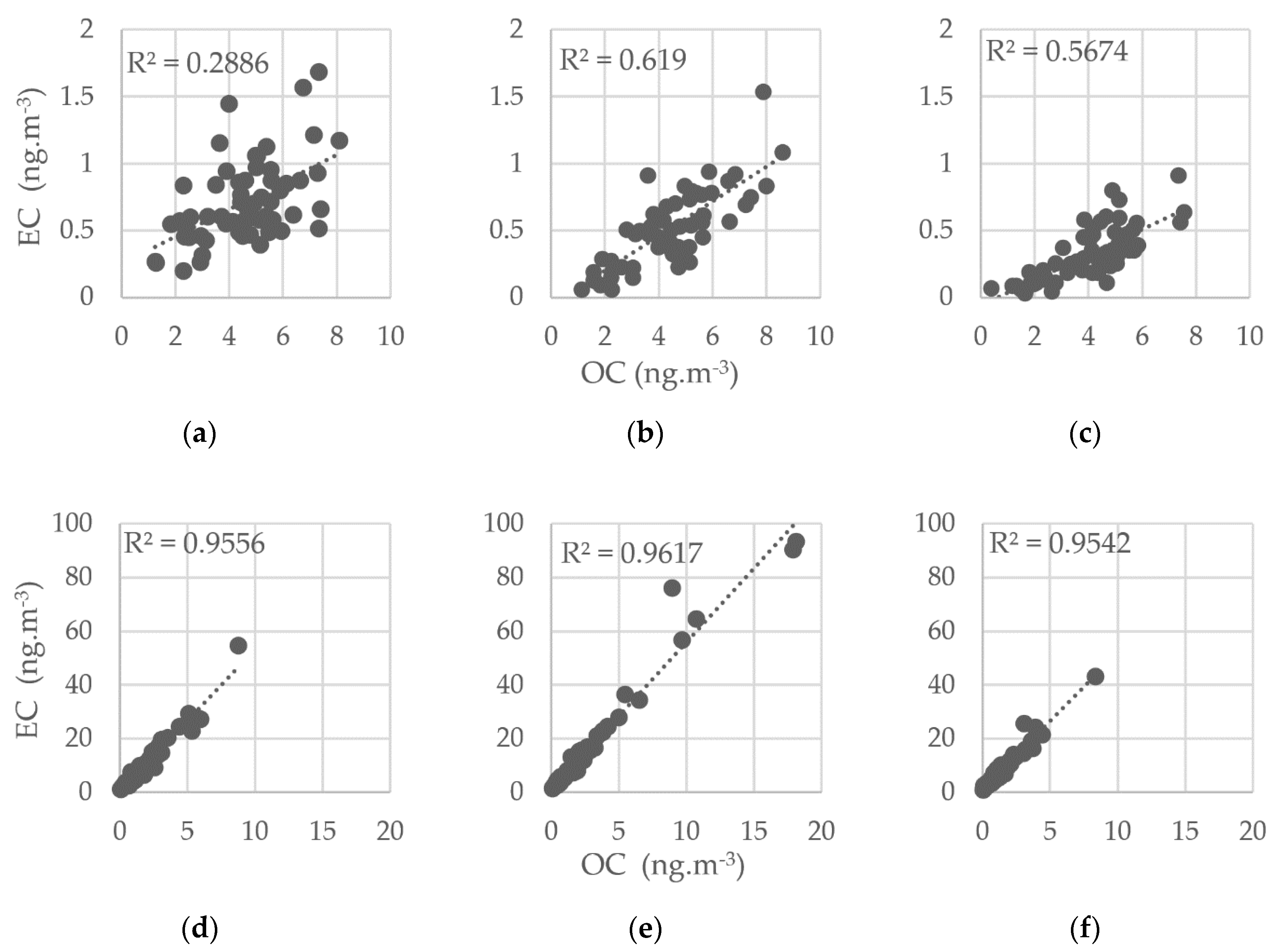101–103), the measured organic carbon summer concentrations are more than twice as high as in the winter (the mean concentration varies in the range of 4.0–4.6 µg.m⁻³ in the summer, depending on the sampling site, and 1.4–1.7 µg.m⁻³ in the winter, respectively), in spite of the fact that both residential heating and traffic emissions are higher in the winter. The measured data thus surprisingly indicate that the main source of organic carbon is neither road traffic nor household heating in the surveyed area. An analysis of the EC/OC ratio in the warm and cold parts of the sampling campaign (Figure 6) clearly shows that winter concentrations are related, with one dominant source type at all three sites (strong EC/OC correlations with R² > 0.95), while summer sources are more complex (0.29 < R² < 0.62). Due to the land use type near the sampling sites (frequent grassy and agricultural areas), and considering the time period of the summer sampling (peak of the flowering season), there is high probability that a significant contribution to the measured summer organic carbon concentrations is of biogenic origin (both primary and secondary aerosols).

A slight correlation has been discovered between the OC summer concentrations and temperature (Figure 7); the strongest is at the Vrchy site (R² = 0.36), which is less polluted by both PM_2.5 and OC. Conversely, the weakest OC versus temperature correlation has been found at the most polluted site, Ropice (R² = 0.13).

Although the EC versus temperature correlations are rather weak, there is an indication that the summer OC concentrations are related to factors which have an effect in the rural rather than in the urban and suburban areas. Thus, the summer OC concentrations are significantly connected with natural emission sources. The apportioning of most of the OC mass into the “Crustal” factor is likely due to similar source areas and the time periods of high biogenic OC and mineral dust contributions. Typically, those are the warm summer days when the low soil moisture and air humidity lead to easy mineral dust and biogenic primary particle resuspension. Meanwhile, the temperature and sunshine are favorable to the formation of biogenic secondary organic aerosol. Due to the above-mentioned reasons and because the summer OC contributions have caused a dominant effect on the overall OC concentration, there has been no way to separate mineral dust and biogenic organic carbon into standalone source profiles in the survey area.

As shown in Figure 6, measured summer EC concentrations were lower than 2 µg.m⁻³, whereas in the winter they reached approx. 50 µg.m⁻³ and, at Ropice even nearly 100 µg.m⁻³. The significant increase of the EC concentration has been detected at all sampling sites. An increase of more than one order of magnitude cannot be explained by the change of weather conditions, especially when considering seasonal wind speed comparison in Section 3.1 (higher wind speed in winter has been discovered). The road traffic emission variation is relatively low during the year and its winter contribution to the EC concentration is thus very likely less than the maximum summer EC concentration (<2 µg.m⁻³). Based on this fact, it is clear that the relative annual road traffic contribution to the total EC mass in Třinecko is very low (in the winter at most several units of percentage). On the contrary, emissions from the coal burning in the old-technology boilers which are the most common residential heating appliances in the surveyed area varies in a wide range during a year. Signs of an incomplete combustion process with the potential for high EC emissions are manifested by the dominant percentage of PAHs in the “residential heating” source profile, consistently with other studies, e.g. [19] (p. 12). Obsolete household heating boilers emitting a lot of soot are thus very likely to be the dominant sources of EC in this region, at least one order of magnitude higher than the road traffic EC contribution. This fact possibly explains why the EC, which is often used a road traffic marker, has not led to the identification of the individual traffic PMF factor in the surveyed area.

In spite of the high winter correlation between EC and OC, these species are separated by the PMF model to the different PMF source profiles. According to the mentioned findings, it is caused by different EC and OC sources in the summer. In the winter, there were acting OC and EC emissions from the residential heating (other sources are negligible compared to this source type). On the contrary, a vast majority of primary biogenic and secondary particles (majority of the summer OC mass) and particles likely originating mainly from traffic (contribution to the EC mass) were the most important in the summer.

4.2. Comparison of the Results of the ED XRF and ICP-MS Methods

The ICP-MS is the reference method for heavy metals measurement in PM_2.5 used within the National Air Quality Monitoring Network according the European and Czech air protection legislation. ED XRF dataset has thus been tested with the aim to verify if it could be a more affordable alternative to the ICP-MS for the source apportionment purposes. Based on the previous comparison of the parallel measurement with ICP-MS (not published in this article), several limitations of ED XRF had been known before its use for PMF modeling. Those are limited species number, significantly higher relative uncertainty and a higher method detection limit of some species compared to ICP-MS. The Table 2; Table 3 show significant concentration differences of some species between ICP-MS and ED XRF dataset, especially in the case of Sb, Ti, V, Cr, and surprisingly, Mg. Based on this and previous comparisons, with caution we have used measured concentrations of the Cd, Cr, Sb, Ti, V, K, Na, S, Si, and Al. Some of these problematic metals has been excluded from the PMF dataset. On the contrary, Cu, Fe, Mn, Pb, Se, and Zn could be considered more reliable.

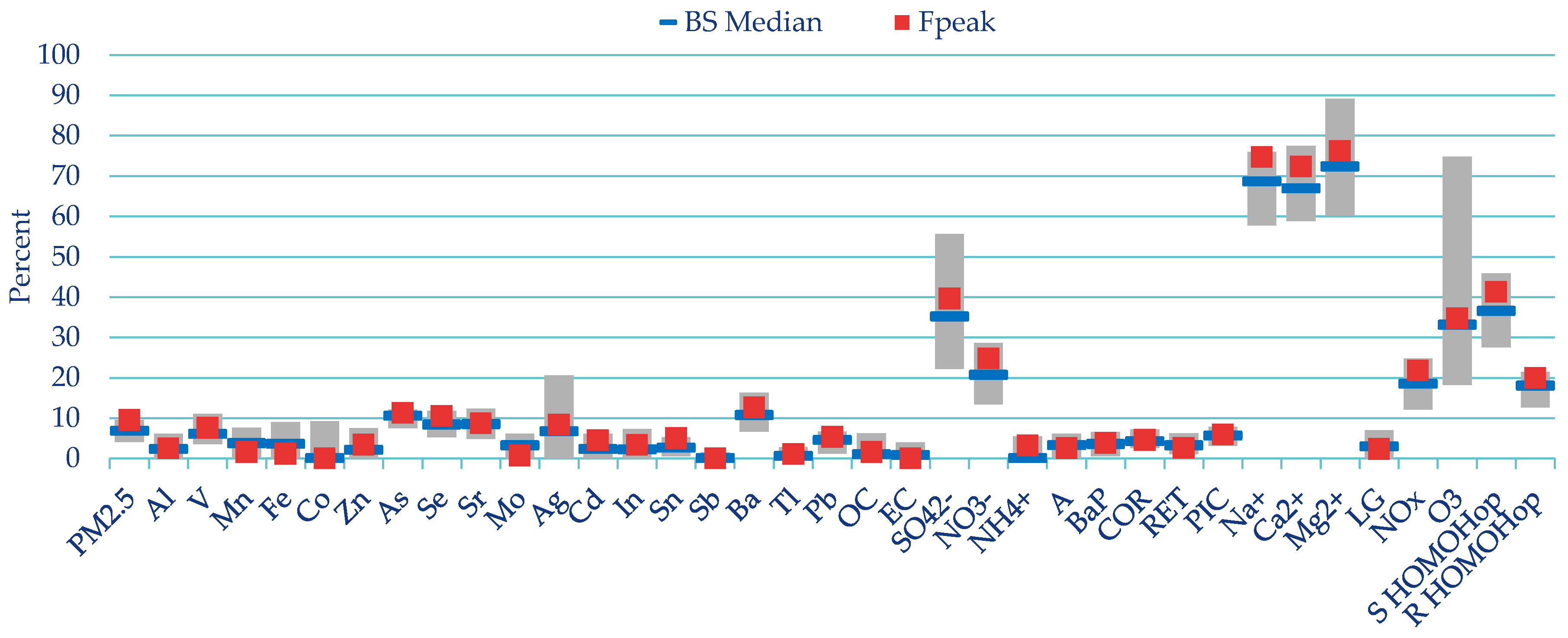
Despite the mentioned ED XRF limitations, the PMF results based on the two different datasets are similar. In both the ED XRF and ICP MS datasets, the uncertainties of the elaborated PMF model according to the U.S. EPA [14] guide criteria are acceptable. The solution found with six factors is stable, with good agreement of the predicted and measured values and with the bootstrap (BS), displacement (DISP), and bootstrap-displacement (BS-DISP) stability tests complying with the guide recommendations [14]. The identified air quality factors and their quantified contributions at different wind directions and speeds correspond well to the location of the real pollution sources.

No significant difference has been detected in the predicative ability of the evaluation based on the ICP-MS and ED XRF datasets, i.e., by means of both methods a solution for the sampling site of Ropice has been found that agrees on the substantial aspects (Figure 8).

The model results using ED XRF and ICP-MS differ significantly only in the case of the regional aerosol and the local heating contribution, whereas in total the two factors are quantitatively identical in both datasets (on the whole, they account for approximately ¾ of the total pollution). The split of the pollution origin between these two factors is always disputable, as in regional aerosol there is also a significant pollution contribution from local residential heating. There is no precise boundary between the local and regional residential heating influences. G-Space Plot indicated a partial mutual link, which thus has a rational basis. All the other identified factors were mutually independent, according to the G-Space Plots analysis. With respect to the goal of the ED XRF and ICP-MS comparison, differences in source contributions up to approximately 5% can be considered as negligible, as they do not change the focus of the main air pollution measures in the research area. It is possible to consider the sensitivity and accuracy of both methods as sufficient for PMF modeling and consecutive recommendations for strategic measures regarding air protection.

4.3. The Use of the Selected Organic Markers

Based on the research information sources mentioned below, some markers have been selected that have proven to be suitable organic molecular tracers for the identification of coal combustion, biomass burning, and vehicular emissions. The concentrations of 19 PAHs, six hopanes, six steranes, and levoglucosan in the PM_2.5 aerosol samples were measured. PAHs are formed mostly from the incomplete combustion of a variety of fuels emitted by different source types, including residential heating, industrial processes, waste incineration, and mobile sources [20,21]. Benzo[a]pyrene is the only PAH that has a legislative limit (1 ng.m⁻³ annual average concentration), and it was used as a marker for carcinogenic risk assessment [22]. The International Agency for Research on Cancer (IARC) classified BaP as an agent carcinogenic to humans (Group 1). Across all three sites, the BaP concentrations were 12–14 times higher for the winter samples (average 3.95 ng.m⁻³) than for the summer samples (average 0.3 ng.m⁻³). The seasonal differences can be explained by decreased residential heating during the warm months and increased photolysis and dispersion of all PAHs. The rest of the measured PAHs had shown fewer seasonal differences (4 –11 times) than BaP, with the exception of BaA (17–21 times), which is highly susceptible to photo-oxidation [20,23].

Concentrations of BaP and BeP are usually similar in fresh emissions [24], but as BaP degrades in the presence of sunlight and strong oxidants in the atmosphere, the BeP/(BeP + BaP) ratio can be used as an index of the aging of aerosol particles [24,25]. During the summer campaign, the ratio BeP/(BeP + BaP) at all three sampling sites was in the range from 0.5 to 0.6, indicating the regional or long-range transport of aerosols. Conversely, in winter, this ratio was less than 0.5 (average 0.4), and that indicates emissions of aerosols from local sources.

Picene was selected as a marker for coal combustion. Furthermore, the diagnostic ratios of the selected hopanes were used to identify the combustion of different types of coal [26]. Hopanes and steranes are present in the lubricating oil used by both gasoline- and diesel-powered motor vehicles. They are considered markers for traffic emissions in the atmosphere [27,28]. On the other hand, only hopanes are present in emissions from coal combustion. The characteristic ratio between concentrations of 22R-17a(H),21b(H)-homohopane and 22S-17a(H),21b(H)-homohopane, known as a homohopane index, can be used for identifying diverse types of coal. For coal combustion, the homohopane index C31αβ[S/(S + R)] is in the range from 0.05 to 0.40 and it increases with the maturity of the coal, 0.05 for lignite, 0.08 for brown coal, 0.20 for sub-bituminous coal, and 0.37 for bituminous coal [26]. The homohopane index obtained for gasoline and diesel emissions ranges from 0.45 to 0.60 [29,30]. Hopane concentrations in the samples were quantified by the key ion m/z 191, and sterane concentrations were quantified by the key ions m/z 217 and 218. Across all three sites, the sterane concentrations were very low or below the detection limit (0.12 ng.m⁻³) in the samples from both the summer and winter campaigns. The most abundant sterane in the summer samples was ααα 20R-Cholestane (average 0.17 ng.m⁻³), and its concentrations within the winter samples were only 2 times higher (average 0.31 ng.m⁻³). Steranes were used as molecular markers for indicating the contribution of vehicular emissions, and their low concentrations indicate a negligible impact of the mobile sources. Like the steranes, the hopane concentrations at all three sites during the summer campaign were exceptionally low, and the homohopane indices were in the range from 0.51 to 0.64, which indicates that hopanes in the summer samples originated mainly from transport emission. During the winter campaign, hopane concentrations were on average 5 times higher than in the summer, and the average homohopane indices for the Kosmos and Ropice sampling sites were 0.36 and 0.34, respectively, which indicates that hopanes in the winter samples were mainly from high-range coal combustion. For the Vrchy site, the homohopane indices were more heterogeneous than at the other two sites, and were in the range from 0.11 to 0.60 (average 0.40). In three samples, the homohopane indices were below 0.20, which is typical for less mature coal. Conversely, in 27 winter samples (almost 50% of the total samples) from the Vrchy site, the homohopane indices were in the range from 0.45 to 0.60, which, according to literature, corresponds to gasoline and diesel emissions. It has been assumed that these could be emissions from the combustion of waste oil or fuel oil due to exceedingly high concentrations of hopanes and steranes in these samples and relatively low concentrations of the measured PAHs. The trend of PAH production during the combustion of various types of fuels in terms of their chemical composition is in the following order: coal > lignite > wood > waste oil > mazut > fuel oil [31].

4.4. Results in the Context of Current Strategies

Among the main documents of air protection in the Czech Republic today are the Air Quality Improvement Programmes, which contain measures for individual regional units of NUTS 2 (Nomenclature of Units for Territorial Statistics, Level 2). For the Třinecko region, the binding measures are stated in the Air Quality Improvement Programme for the Agglomeration of Ostrava/Karviná/Frýdek-Místek CZ08A [7], the analytical part of which was elaborated using the CAMx chemical transport model.

Based on the established wind direction and speed during the campaigns, it is possible to state that these meteorological conditions, which are one of the main factors influencing the dispersion conditions, correspond well to the long-term average measured at the nearest neighboring sites of the National Air Quality Monitoring Network. It is thus possible to consider that the acquired results are sufficiently representational for a longer period of time and that they can be used for a proposal for strategic measures.

The source apportionment by means of PMF, including an approximate determination of the main source areas of the secondary aerosol, provides new arguments for the prioritization of measures that have so far been missing in the strategic documents relevant to the Třinecko region.

As stated in the previous studies [32] (p. 6), due to the different definition of their sources, comparing the source apportionment output of receptor models and the chemical transport model is not straightforward. Nevertheless, it is evident that the PMF results correspond to the CAMx results in the analytical part of the mentioned strategic document in its main priorities. According to both modeling methods, the main cause of the above-limit pollution by PM_2.5 in Třinecko is individual residential heating, followed by secondary aerosol and transport from abroad. Compared to existing analyses using chemical transport models, the PMF modeling results show a significantly higher influence of local sources (especially residential heating), whereas in the case of the secondary aerosol and transport from abroad, the situation is the opposite. The contribution of transborder pollution is assessed as significant but not high by the PMF model. According to the PMF model, the most significant part of air pollution by PM_2.5 is of local origin, i.e., it comes predominantly from an area within units of km from the assessed sites.

5. Conclusions

The aim of the research documented in the presented article was to contribute to a better understanding of the relations among emissions, pollution transport, and ambient air PM_2.5 concentrations in Třinecko by source apportionment using positive matrix factorization (PMF). At the three assessed sites, six main factors have been identified (two types of residential heating, regional primary and secondary aerosol sources, resuspended dust and biogenic detritus, long-range transport, and iron and steel production). In substantial aspects, the results correspond to earlier analyses carried out for air protection strategic plans. However, they also bring some important corrections. This is true especially when it comes to the discovery that the most significant pollution contribution falls under local sources, whereas pollution transport from more remote areas, including abroad, is less significant.

It is possible to consider a significant decrease of primary emissions of PM, polycyclic aromatic hydrocarbons, and sulfur dioxide from individual residential heating, which create the greatest air pollution contribution, and the associated health hazards as the main priority of air protection in Třinecko. Directing measures to this source type will support a decrease in the influence of the second most significant pollution type, which is “regional aerosol”.

In this respect, support of traffic measures, from the point of view of air protection, is less important nowadays. Although some interpretation problems with traffic contribution quantification by the PMF have been found, there are no doubts about its minor role, especially considering other source apportionment approaches, including the recent CAMx model which has been provided for planning the strategy measures. Due to the PMF results accordance with the mentioned independent alternative source apportionment method, the traffic measures in Třinecko should have been limited to specific activities at particular locations where it is possible to demonstrably prove an acceptable ratio of costs to air quality improvement. Other factors influencing the air quality at present are not a regional priority in Třinecko now. Measures focusing on them can only be effective locally.