Article

Multi-Model Ensemble Sub-Seasonal Forecasting of Precipitation over the Maritime Continent in Boreal Summer

1
Plateau Atmosphere and Environment Key Laboratory of Sichuan Province, College of Atmospheric Science, Chengdu University of Information Technology, Chengdu 610225, China
2
State Key Laboratory of Severe Weather, Chinese Academy of Meteorological Sciences, Beijing 100081, China
3
Laboratory for Climate Studies & CMA-NJU Joint Laboratory for Climate Prediction Studies, National Climate Center, China Meteorological Administration, Beijing 100081, China
4
Climate Change Research Center, Institute of Atmospheric Physics, and Nansen–Zhu International Research Centre, Chinese Academy of Sciences, Beijing 100029, China
5
Department of Atmospheric and Oceanic Sciences & Institute of Atmospheric Sciences, Fudan University, Shanghai 200433, China
*
Author to whom correspondence should be addressed.
Atmosphere 2020, 11(5), 515; https://doi.org/10.3390/atmos11050515
Submission received: 7 April 2020 / Revised: 28 April 2020 / Accepted: 13 May 2020 / Published: 16 May 2020
(This article belongs to the Section Meteorology)

Abstract

:
The Maritime Continent (MC) is a critical region with unique geographical conditions and significant monsoon activities that plays a vital role in global climate variation. In this study, the weekly prediction of precipitation over the MC during boreal summer (from May to September) was analyzed using the 12-year reforecasts data from five Sub-seasonal to Seasonal (S2S) models, including the China Meteorological Administration (CMA), the European Centre for Medium-Range Weather Forecasts (ECMWF), Environment and Climate Change Canada (ECCC), the National Centers for Environmental Prediction (NCEP), and the Met Office (UKMO). The result shows that, compared with the individual models, our newly derived median multi-model ensemble (MME) can significantly improve the prediction skill of sub-seasonal precipitation in the MC. Both the Temporal Correlation Coefficient (TCC) skill and the Pattern Correlation Coefficient (PCC) skill reached 0.6 in lead week 1, dropped the following week, did not exceed 0.2 in lead week 3, and then lost their significance. The results show higher prediction skill near the Equator than in the north at 10° N. It is difficult to make effective predictions with the models beyond three weeks. The prediction ability of the median MME improves significantly as the total number of model members increases. The prediction performance of the median MME depends not only on the diversity of models but also on the number of model members. Moreover, the prediction skill is particularly sensitive to the intensity and phase of Boreal Summer Intraseasonal Oscillation 1 (BSISO1) with the highest skills appearing at initial phases 1 and 5.

1. Introduction

The Maritime Continent (MC), located at the junction of the Indian Ocean and the Pacific Ocean, consists of several islands and shallow seas [1]. It is an essential area in the Northern and Southern Hemispheres that interacts through the cross-equatorial flow. Asian–Australian monsoon activity is closely related to atmospheric changes in this area [2]. Due to the distinct geographical conditions and remarkable monsoon activities, MC plays a critical role in surrounding and even global climate variations [3]. Convection in the MC region features multi-scale spatial-temporal activities [4]. Since the 1960s, many studies have been conducted on the climatic features and impacts of the MC region [5,6,7,8,9].
The sub-seasonal to seasonal (S2S) prediction (the so called “desert of predictability”) is an urgent problem that necessarily needs to be solved. On one hand, S2S fills in the gap between medium-to-long range weather forecast and seasonal prediction. On the other hand, the improvement of S2S forecast for extreme events will contribute to the prevention of climatic disaster and economic loss [10]. S2S prediction lies between weather forecast and climate prediction, in which initial conditions as well as boundary conditions are extremely important [11,12,13,14]. The study [15] has shown that there are several potential sources of predictability that contribute to this timescale, such as the intraseasonal oscillation (ISO), El Nino Southern Oscillation (ENSO), soil moisture, snow cover, sea ice, stratosphere–troposphere interaction, etc. [16,17,18,19,20]. Madden–Julian Oscillation (MJO) is the primary intraseasonal mode of organized convective activity in tropical regions, and it significantly influences on the global monsoon and also has a considerable impact on the middle and high latitudes [21,22,23]. In addition, the Boreal Summer Intraseasonal Oscillation (BSISO) has become the dominant mode during boreal summer [24,25].
The S2S Prediction Project and associated database [26] have already been jointly established by the World Weather Research Programme (WWRP)/World Climate Research Programme (WCRP) to promote S2S research and operational prediction [27]. Studies based on S2S model outputs have been carried out recently. The MJO prediction skill of the majority of S2S models has exceeded 20 days. Although models have significantly improved the predictions of MJO and major climatic phenomena [28,29], they tend to underestimate the intensity and propagation speed of MJO, and it is difficult to propagate MJO across the MC [30]. Some studies also show model assessment for monsoons, extreme events, and tropical cyclones (TCs). It is shown that models have some capability in reproducing the atmospheric dynamics that influence monsoon variability, predicting the onset, evolution, and decay of some large-scale extreme events and predicting the occurrence of basin-wide TCs. The eye-catching performance of the European Centre for Medium-Range Weather Forecasts (ECMWF) model is no surprise [31,32,33]. Some previous studies have focused on the comparison of multi-model performances and the evaluation of predictability sources [34,35,36,37,38].
The multi-model ensemble (MME) is found to be an effective approach to improve weather [39,40] and climate prediction [41,42]. MME can greatly reduce the uncertainty of the forecast and increases its reliability compared to single-model ensemble prediction [43,44]. To better promote the development of MME forecast for short-term climate (seasonal to interannual) prediction, several research projects, such as ENSEMBLES [45], the US National Multi-Model Ensemble (NMME) [46], and China MME (CMME) [47] have been launched. The implementations of the MME technique have effectively improved the prediction of weather (e.g., tropical cyclones) and climate variability on both seasonal [48,49,50,51] and sub-seasonal timescales [52,53]. With the S2S database, Specq et al. [54] first attempted to assess the balanced MME forecast skill of precipitation over the southwest tropical Pacific at the sub-seasonal timescale.
Compared to well-implemented weather and seasonal forecasts, less attention has been paid to sub-seasonal prediction in general, much less the precipitation in the MC. Studying precipitation in the MC contributes to raising awareness of climate evolution and provides scientific reference for precipitation prediction. This paper aims at constructing MME forecast and revealing the predictability of sub-seasonal precipitation during boreal summer in the MC. This paper is organized as follows: models, data, and methods are introduced in Section 2; in Section 3, we focus on the prediction skill of individual models and the MME; the association of MME prediction with MJO and BSISO is analyzed in Section 4. The summary and discussion are given in Section 5.

2. Models, Data, and Methods

2.1. Data

Data products generated from five S2S models are used in this study, namely the China Meteorological Administration (CMA), ECMWF, Environment and Climate Change Canada (ECCC), the National Centers for Environmental Prediction (NCEP), and the Met Office (UKMO). Boreal summer is defined as May–June–July–August–September (MJJAS). Noting that the S2S database was not produced following a consistent protocol, basic information on the 5 models is shown in Table 1.
The analysis period of the five model outputs is unified to 1999–2010 MJJAS. Each month consists of four start dates; the start dates of May are shown in Figure 1. The observational daily precipitation data were provided by the Global Precipitation Climatology Project (GPCP) [55] with a horizontal resolution of 1° × 1° latitude/longitude. As part of the WCRP, the GPCP aims to observe and estimate global precipitation. It is based on more than 6000 routine surface observation stations and integrates the satellite observational results. For the purpose of comparing the results of models and observation in the MC, model and observational data were consistently interpolated onto the 2.5° × 2.5° grid by using the bilinear interpolation. In order to examine the relationship between sub-seasonal precipitation and ISO in the MC, the Real-time Multivariate MJO (RMM) index [56,57] and the BSISO index [58] were also used. The MC domain was taken as 90° E–150° E, 10° S–20° N.

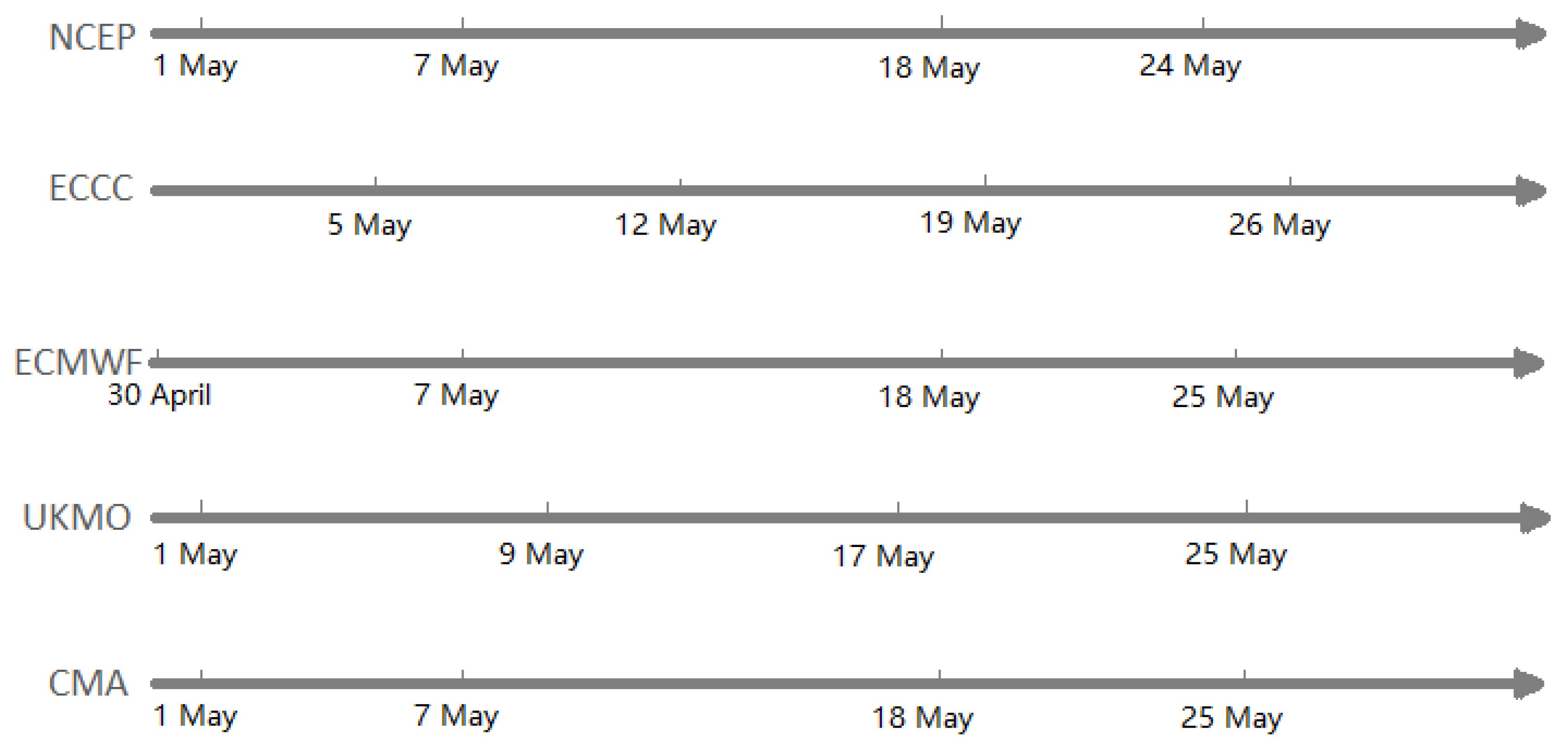
2.2. Construction of MME

As can be seen from Table 1 and Figure 1, it is obvious that the five S2S models do not follow an agreed-upon protocol; there is also no standard construction of the MME due to the start dates of each model being different. Thus, the construction of an S2S-MME is quite necessary but a challenging issue. This study tries to make such an S2S-MME possible by constructing a median MME instead of traditional arithmetic MME (e.g., Ren et al. [47]), also referring to the work of Specq et al. [54]. We think that median MME is a better method in terms of different S2S models. The construction of the MME refers to the start date of the CMA. Table 2 is an example of constructing MME with three different start dates (30 April, 1 May, 5 May) for the forecast of the target week (6–12 May). In this example, the CMA’s lead-a-week forecast for 6 to 12 May can choose 1 May as the start date. For the ECCC, the nearest start date is 5 May. Therefore, a given forecast target week may correspond to different start dates for different models.
The number of ensemble members is not exactly the same for each model (CMA, ECCC, and NCEP each have 4 members, ECMWF has 11 members, and UKMO has 3 members); therefore, a uniform number of members was selected to construct MME. In this study, we considered constructing MMEs of 15, 10, and 5 members (including 3, 2, and 1 from each model), respectively. The median performance ensemble of each model was selected to construct the MME. For example, CMA has four ensemble members (a, b, c, d), and thus we can get four ensembles (abc, abd, acd, bcd) constructed by three members. We chose the median of four ensembles as the ensemble of CMA, and the MME was composed of the respective median ensemble of five models.

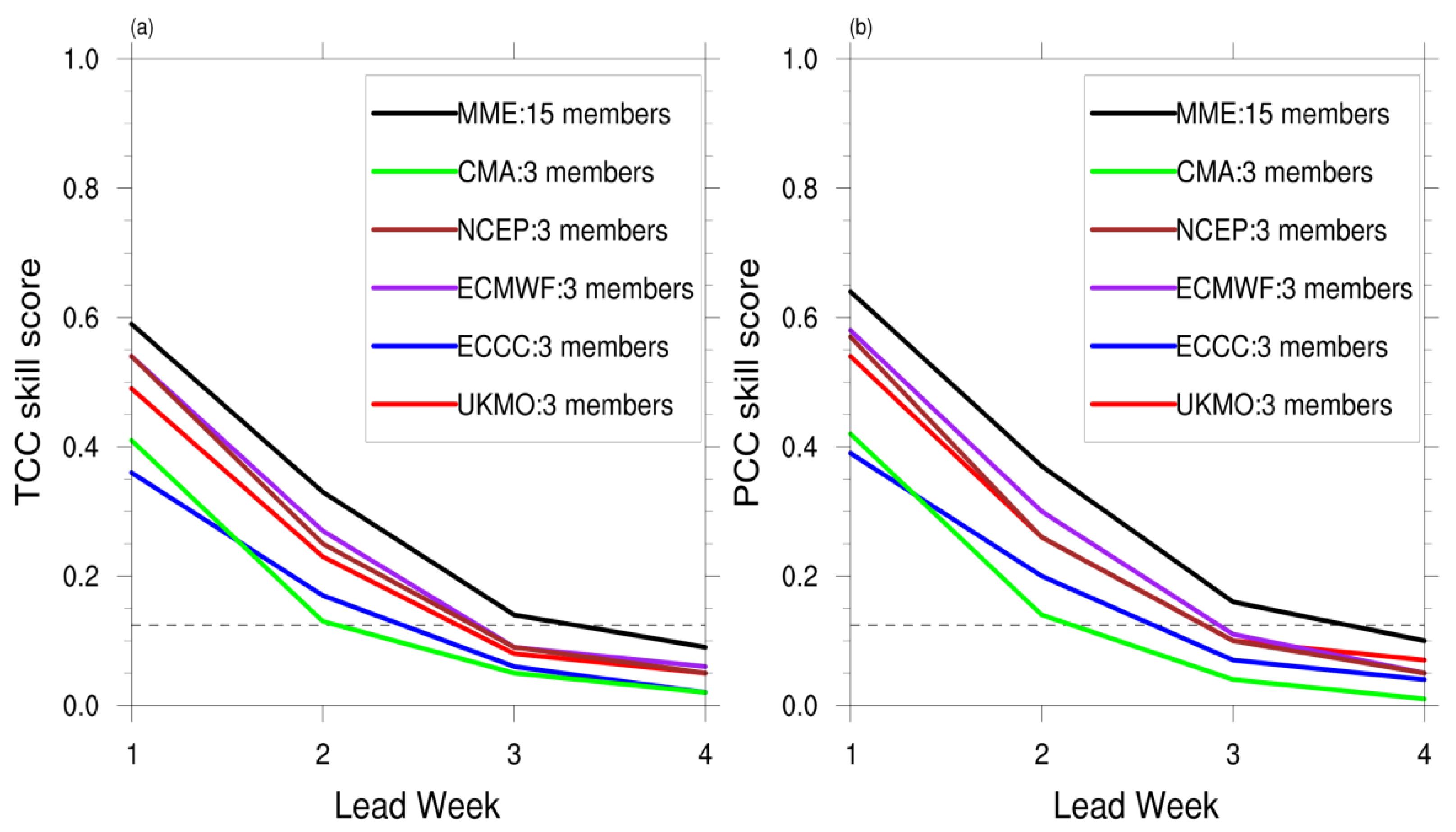
2.3. Forecasting Skill Metrics

In this paper, WMO-recommended standards are used to evaluate prediction performance [59]. The Temporal Correlation Coefficient (TCC) is used to measure the prediction skill. TCC can represent the temporal agreement of model forecast statistical significance and is able to acquire a distribution of prediction skill by calculating the TCC of each grid point. The calculation formation is given as:
T C C i = j = 1 N ( x i , j x ¯ i ) ( y j y ¯ ) j = 1 N ( x i , j x ¯ i ) 2 j = 1 N ( y j y ¯ ) 2 ,
where i denotes the start date and j denotes the target week. x i , j represents the predicted week j mean anomalies starting on date i , and x ¯ i represents the average of predicted mean anomalies starting on date i of each week. y i expresses the observation anomalies in week j , and y ¯ expresses the average of y j . N is the number of time samples. The range of TCC is between −1 and 1, and the closer the TCC is to 1, the higher the forecasting skill.
Unlike TCC, the Pattern Correlation Coefficient (PCC) reflects the spatial agreement of the model forecast and acquires a variation of prediction skill by calculating PCC of different times. The calculation formula is as follows:
P C C j = i = 1 M Δ x i , j Δ y i , j j = 1 M Δ x i . j 2 j = 1 M Δ y i , j 2 ,
where j denotes the target week and i denotes the grid point. Δ x i , j and Δ y i , j represent the predicted and observational week j mean anomalies on grid i , respectively. M is the total number of the grid point over the MC. The PCC also ranges from −1 to 1. A larger PCC indicates a more consistent spatial pattern between model forecast and observation.

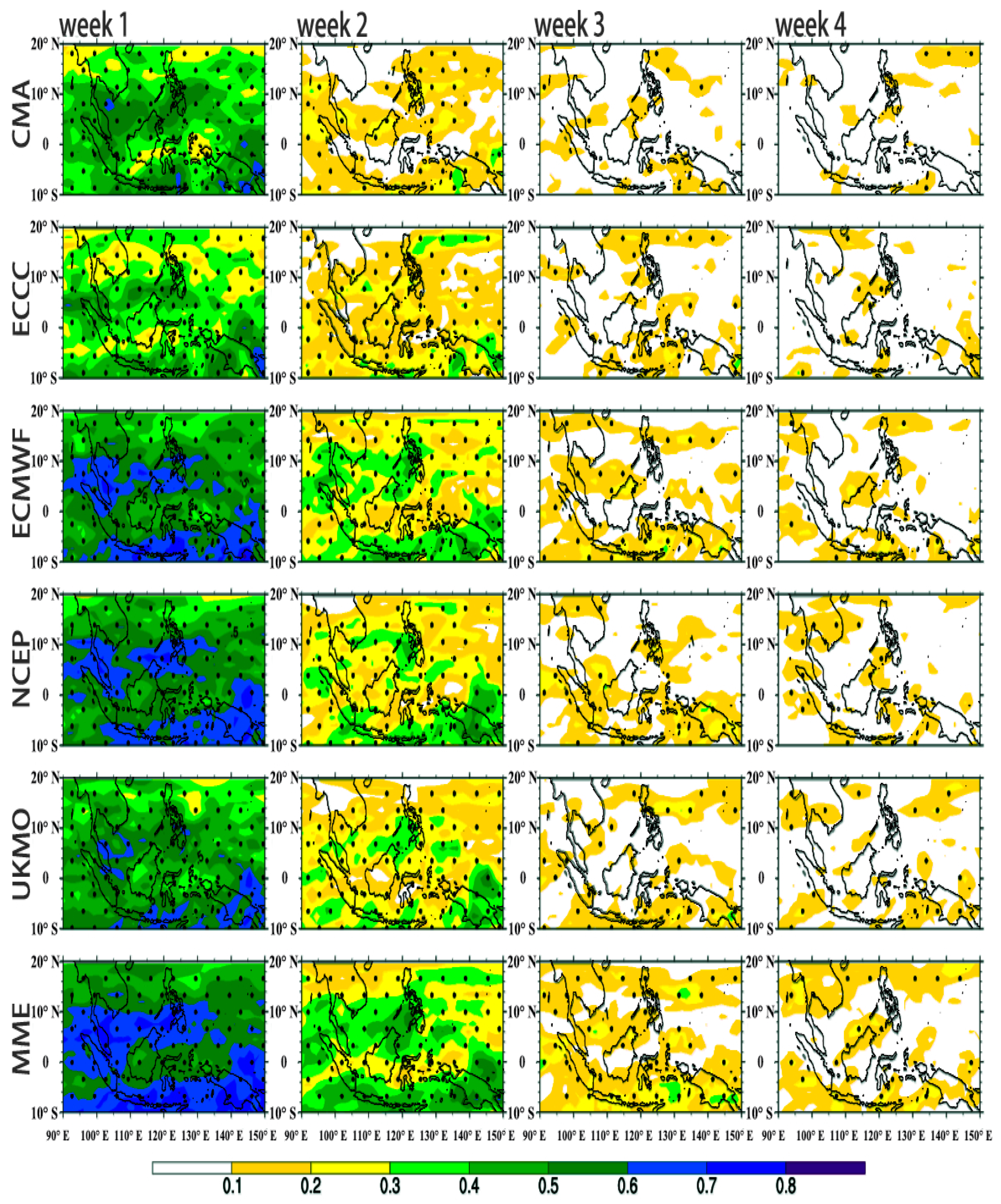
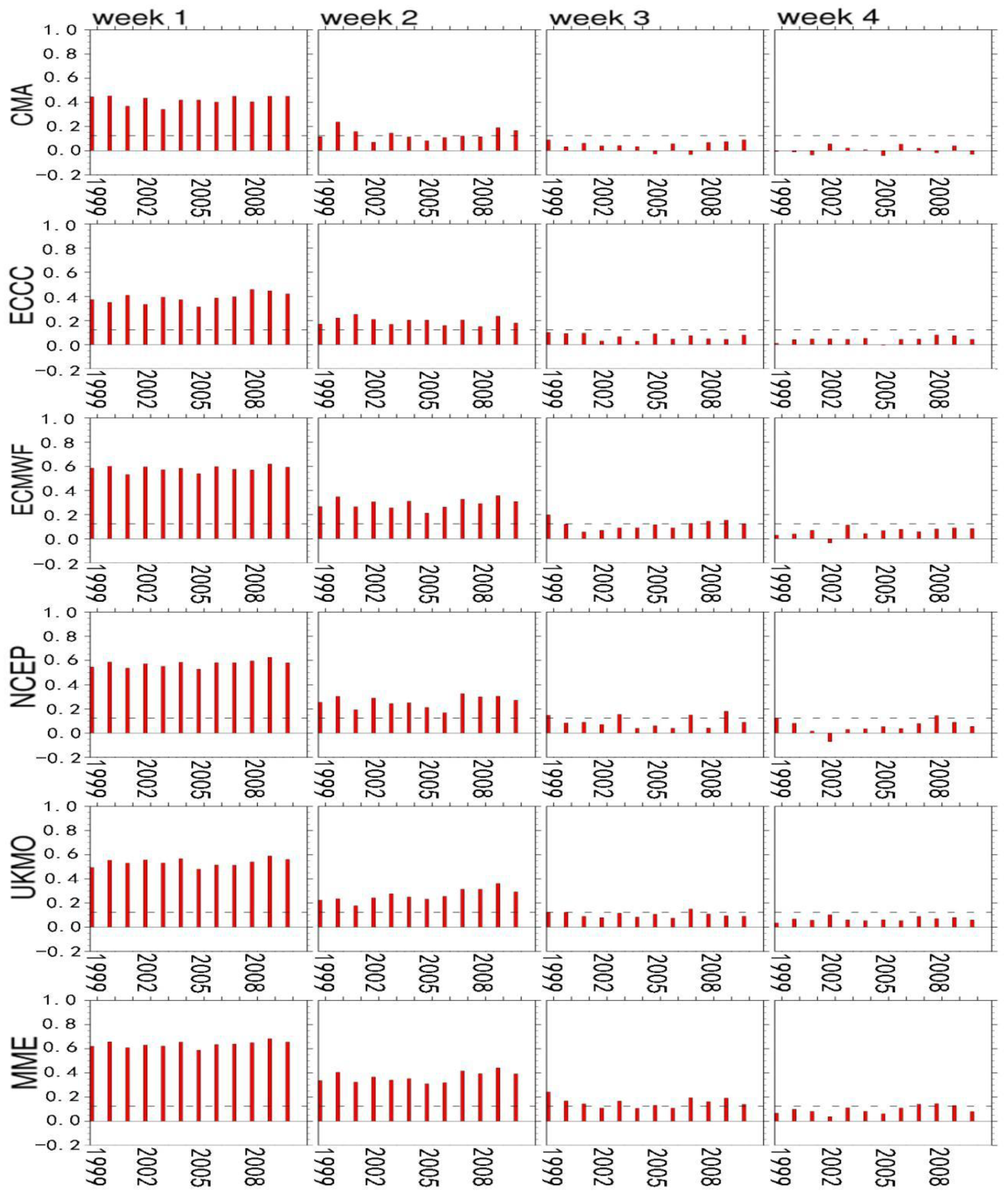
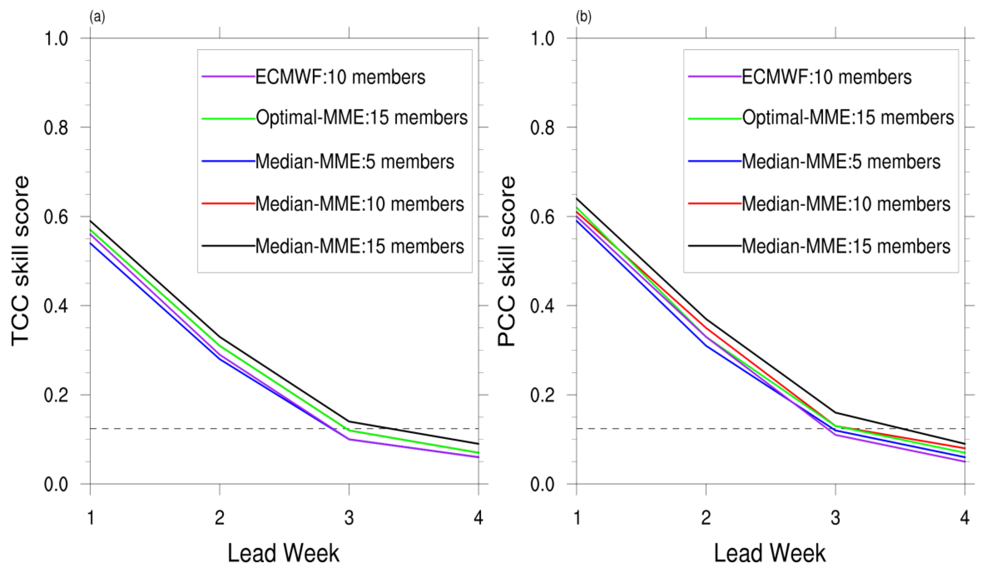
3. Prediction Skills of Individual Models and MME

The TCC skills of the five individual models and the MME are shown in Figure 2. The ensemble member of each model is unified for three members. The result shows that the TCC skill of each model decreases with the increase in lead time. During lead week 1, TCC of most of the MC regions is greater than 0.4. After lead week 1, prediction skill rapidly drops. The prediction skill of the MME is significantly larger than the single model, and most regions can still reach above 0.3 in lead week 2. Compared with the single model, the MME still shows significant skills in lead week 3, and all models lose their prediction ability in lead week 4. The performance of the ECMWF and NCEP is relatively better than the other three models. Furthermore, the results show that prediction skill by the Equator tends to be higher than that north of the Equator.
The prediction skill of the MC is significantly higher than those of the middle and high latitudes [60]. As shown in the MME, high-skill regions are concentrated near the Equator over ocean; Sumatra, Kalimantan and the Philippines have higher skill over land. There is no significant difference through analyzing the spatial average of the TCC skill over the ocean and the land. Interestingly, the skill over ocean is more significant after lead week 3, which indicates that the skill over ocean is higher compared to that over land.
Figure 3 shows the interannual variations of the PCC skills for the five individual models and the MME. Similar to TCC, the PCC skill of each model decreases with the increase in lead time, and the prediction skill of the MME is relatively higher than individual models. The PCC skills of all models drop significantly in lead week 3 but are still positive for most cases, even for lead week 4.
Focusing on the overall prediction skill in the MC, the spatial average (90° E–150° E, 10° S–20° N) of the TCC and time average (1999–2010) of the PCC are shown in Figure 4. The skills are relatively high in lead week 1 and rapidly drop in lead week 2. The ECMWF has the best performance, with the NCEP and UKMO very close behind, followed by the CMA and ECCC models. MME can effectively improve the forecast skill and is still significant in lead week 3, although the skills of all models are not significant. The forecast skill after 3 weeks decreases slowly and is not statistically significant as the lead week increases. This indicates that the MME lost its prediction skill after three weeks. In addition, the time average of the PCC is relatively higher than the spatial average of the TCC, indicating that the model is better at capturing the spatial distribution characteristics of precipitation relative to its temporal evolution.
To explore the impact of ensemble members on the prediction skill of the MME, MMEs of 5, 10, and 15 members were constructed. We call this the median MME because the MMEs are constructed with five models, as shown in Figure 5. The prediction skill of the MME relies on ensemble members, with more members denoting higher skill when the number of models is constant, which is reflected by both the TCC and PCC skills. To compare the prediction ability of the MME with that of the individual model under the same number of members, the ECMWF model of 10 members ensemble was also plotted. Although the ECMWF model has excellent performance (consistent with the results in Figure 2, Figure 3 and Figure 4), the MME can still improve the prediction ability.
In order to explore the impact of the diversity of models on the prediction ability of the MME, we constructed two types of 15-member MMEs for comparison. The ECMWF model with 11 members and the NCEP model with four members were selected to construct a 15-member MME, known as the optimal MME. As shown in Figure 5, impressively, the median MME skill is larger than the optimal MME. The diversity of models significantly contributes to the performance of the MME than the single model with better performance. This shows that the number and the diversity of models with a certain number of ensemble members needed to be taken into consideration when constructing an MME. Some suitable ensemble methods also have a great impact on improving the prediction performance of the MME, which is also worth further exploring.

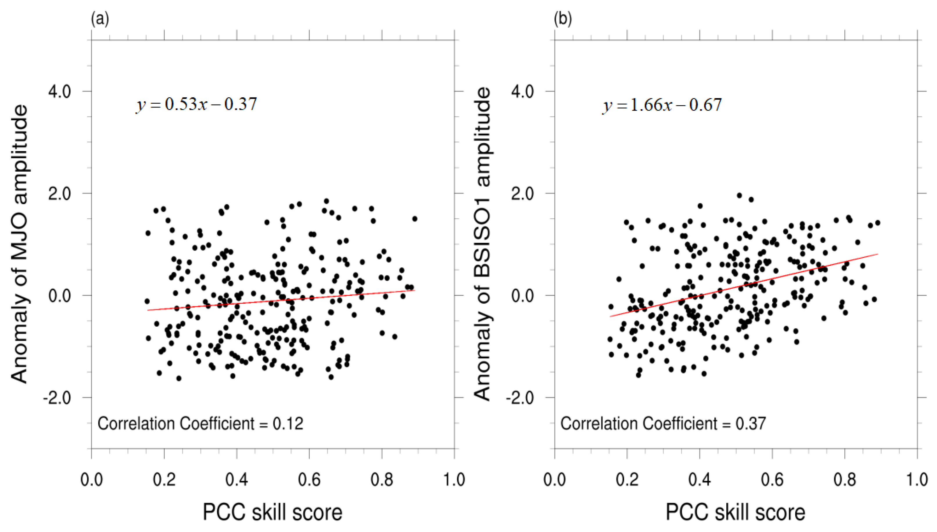
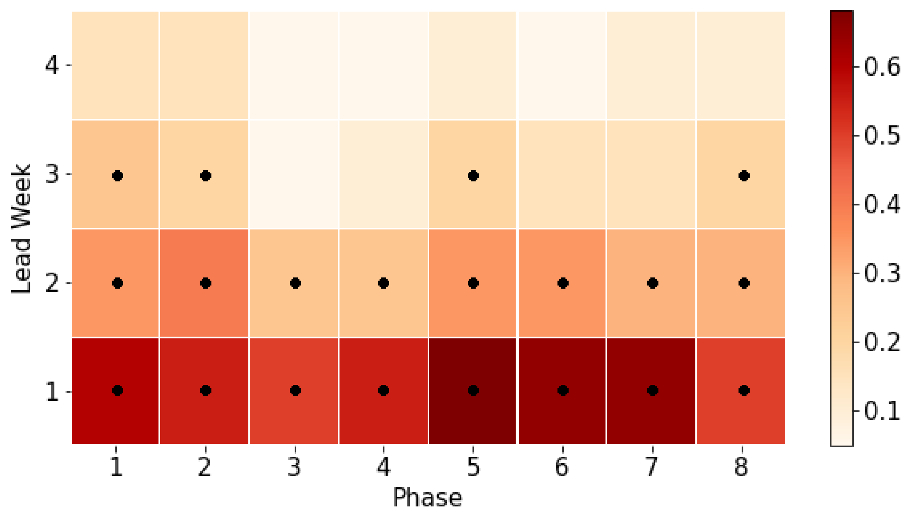
4. Association of MME Prediction with MJO and BSISO

ISO plays a crucial role in the prediction of sub-seasonal timescales. Madden and Julian [61,62] defined the tropical atmospheric low-frequency oscillation MJO as the most significant ISO in tropical regions, especially in winter. The MJO convection signal is strongest over the tropical Indian Ocean and Western Pacific. It propagates eastward with a speed of 5 m s−1, circulating the globe within a period of 30–60 days. The MJO index [56] can visually reflect the position and propagation of MJO according to the two-dimensional spatial phase diagram composed of RMM.
In addition to the eastward propagation, ISO in the boreal summer also has a significant northward propagating component, which has been popularly called BSISO [63]. The BSISO index proposed by Lee et al. [25] include BSISO1 and BSISO2 indices, which describe both the eastward and northward movements of BSISO within a period of 10–60 days. The BSISO1 index describes the typical northward and the eastward propagation within a period of 30 to 60 days.
The PCC skill of precipitation in lead week 1 was scattered against the amplitudes of BSISO1 and MJO to explore the correlation between the prediction skill of the 15-member median MME and the ISO intensity by linear regression. As shown in Figure 6, the prediction skill of the MME is weakly positively correlated with MJO intensity, and the correlation coefficient is around 0.12. Compared with MJO, BSISO1 has a prominent correlation relationship with a correlation coefficient of 0.37. It shows that the amplitude of BSISO1 has a significant influence on weekly precipitation prediction; in other words, BSISO1 provides important sub-seasonal predictability for precipitation in the MC.
In order to further explore the relationship between BSISO1 phase and MME prediction, the prediction skill for different BSISO1 phases is displayed in Figure 7. The PCC skill for each phase is the highest in lead week 1, and skill decreases with the increase in lead week. The skill of phase 1 and phase 5 is relatively high and declines slowly after lead week 2, indicating that there is relatively high predictability when initiated in phase 1 and phase 5. The skill initiated in phase 3 is the lowest.
Since phase 1 and phase 5 of BSISO1 have relatively high predictability, the two phases with the prominent prediction skill are as shown in Figure 8 and Figure 9 skill of phase 1 is higher). In phase 1 (Figure 8), during the 1–4 weeks of observation, there is a rain belt between the west of Sumatra and Kalimantan Island, and the dry area north of 10° N shrinks after week 1. There is a trend of eastward movement over time; this trend can be basically simulated in the first two weeks, and there is some simulation capability for the dry regions of the eastern Philippines, but it is difficult to simulate the west of the Philippines (Figure 8f,g). Furthermore, models in median MME failed to effectively simulate the propagation and position of convection after week 3.
In phase 5 (Figure 9), the convection occurs near the Bay of Bengal to the South China Sea and the northwest Pacific region in the north of New Guinea. There are significant dry regions in Kalimantan Island and west of Sumatra. Convection tends to weaken and propagates toward the northeast with the increase in lead week. However, the simulation ability is weak and lasts for just two weeks. The models in the median MME can capture the convection cells in mainland Southeast Asia, near the South China Sea and east of the Philippines, but, in the Indochina Peninsula, the models tend to underestimate precipitation in lead week 1 and overestimate precipitation in lead week 2. Moreover, the capture of the eastward signal lags for models in the median MME (Figure 9c,g).

5. Summary and Discussions

In this paper, 12-year (1999–2010) reforecasts from five S2S models, including CMA, ECMWF, ECCC, NCEP, and UKMO, are used to study the sub-seasonal predictability of the precipitation of the MC during the boreal summer. Based on the 20 start dates (May–September), a median MME was constructed, and the multi-week prediction of precipitation in the MC was evaluated based on TCC and PCC skill scores. The relationship between prediction skill in this region and the MJO and BSISO is examined.
It is found that there are significant differences between the abilities of the five individual models and their Multi-model ensemble. The prediction skills of all models decrease with the increasing the lead week. The performances of ECMWF and NCEP are relatively better than those of the other models. The prediction skill of the MME is significantly larger than any individual models. According to the spatial distribution of the TCC skill, the prediction skill is higher in low latitudes than that in high latitudes, and the skill over ocean is more significant than that over land after lead week 3. PCC skills exhibit significantly interannual variations. Both skill measures are relatively high in lead week 1, then rapidly drop in lead week 2. In lead week 3, the skills of all models are not significant except for the MME. Therefore, the models have no useful prediction skill for summer precipitation in the MC after 3 weeks.
The number of ensemble members has a significant impact on the prediction skill of the median MME, with more members denoting higher skill when the number of models is constant. When ensemble members are constant, median MME can improve the prediction ability compared with the best-performing model. It is obvious in both that the improvement in prediction skill comes from the error elimination of the individual model. Furthermore, the diversity of models significantly contributes to the performance of the median MME compared to the individual model with better performance, so the diversity of models should be given priority to construct the MME, and there is no doubt that the importance of both is worth exploring further.
The intensity of ISO has a significant influence on weekly precipitation prediction; this characteristic is especially true with the BSISO. Precipitation prediction skills for different BSISO1 phases are also quite different, and skill decreases with the increase in lead week. There is relatively high predictability in phase 1 and phase 5. In phase 1, a trend of eastward movement can be basically simulated in the first two weeks, but models in the median MME failed to effectively simulate the propagation and position of convection after week 3. In phase 5, models in the median MME can basically simulate the convection cells in mainland Southeast Asia, near the South China Sea and east of the Philippines, within 2 weeks, based on a composite analysis for 1-4 weeks of precipitation anomalies. In the Indochina Peninsula, the models tend to underestimate precipitation anomalies in lead week 1 and overestimate precipitation anomalies in lead week 2. Moreover, the capture of eastward the signal lags for models in the median MME.
Although we have demonstrated that the MME is an effective way to improve the prediction skill of sub-seasonal precipitation in the MC, a considerable amount of further research is warranted. The construction of the MME requires the participation of more S2S models. The proportion of excellent models and the diversity of models require further research when constructing the MME. The key physical processes [64] and initial value problems [65] of the S2S models still need in-depth diagnosis and analysis. Considering the interaction between sub-seasonal scale and other scale signals is also an important direction to improve short-term climate prediction [66]. Furthermore, applying dynamic-statistical prediction methods [67,68,69,70,71] on the base of the MME is necessary for the improvement of S2S prediction.

Author Contributions

Conceptualization, H.-L.R., J.-X.F. and Q.-L.C.; methodology, H.-L.R. and J.-X.F.; data curation, W.-H.J.; writing—original draft preparation, Y.W.; writing—review and editing, H.-L.R., F.Z., J.-X.F. and J.W.; visualization, Y.W.; project administration, H.-L.R. and P.-Q.Z.; funding acquisition, H.-L.R. and J.W. All authors have read and agreed to the published version of the manuscript.

Funding

This study was jointly supported by sponsored by the National Key Research and Development Program of China on Monitoring, Early Warning and Prevention of Major Natural Disaster (Grant Nos. 2017YFC1502302, 2018YFC1505906), the National Natural Science Foundation of China (Grant Nos. 41775066, 41905067, 41375062).

Conflicts of Interest

The authors declare no conflict of interest.

References

  1. Ramage, C.S. Role of tropical “Maritime Continent” in the atmospheric circulation. Mon. Weather Rev. 1968, 96, 365–370. [Google Scholar] [CrossRef] [Green Version]
  2. McBride, J.L. Indonesia, Papua New Guinea, and tropical Australia: The southern hemisphere monsoon, in meteorology of the Southern Hemisphere. Am. Meteorol. Soc. 1998, 27, 89–100. [Google Scholar] [CrossRef]
  3. Neale, R.; Slingo, J. The Maritime continent and its role in the global climate: A GCM study. J. Clim. 2003, 16, 834–848. [Google Scholar] [CrossRef]
  4. Meehl, G.A. The annual cycle and interannual variability in the tropical Pacific and Indian ocean regions. Mon. Weather Rev. 1987, 115, 27–50. [Google Scholar] [CrossRef] [Green Version]
  5. McBride, J.L.; Haylock, M.R.; Nicholls, N. Relationships between the Maritime Continent heat source and the EI Nino-Southern Oscillation phenomenon. J. Clim. 2003, 16, 2905–2914. [Google Scholar] [CrossRef] [Green Version]
  6. Chang, C.P.; Harr, P.A.; Chen, H.J. Synoptic disturbances over the equatorial South China sea and Western Maritime Continent during boreal winter. Mon. Weather Rev. 2005, 133, 489–503. [Google Scholar] [CrossRef]
  7. Qian, W.H.; Lee, D.K. Seasonal march of Asian summer monsoon. Int. J. Climatol. 2000, 20, 1371–1386. [Google Scholar] [CrossRef]
  8. Qian, J.H. Why precipitation is mostly concentrated over islands in the Maritime Continent. J. Atmos. Sci. 2008, 65, 1428–1441. [Google Scholar] [CrossRef]
  9. Wang, B.; Ding, Q.H. Global monsoon: Dominant mode of annual variation in the tropics. Dyn. Atmos. Ocean. 2008, 44, 165–183. [Google Scholar] [CrossRef]
  10. Materia, S.; Muñoz, Á.G.; Álvarez-Castro, M.C.; Mason, S.J.; Vitart, F.; Gualdi, S. Multimodel Subseasonal Forecasts of Spring Cold Spells: Potential Value for the Hazelnut Agribusiness. Weather. Forecast. 2020, 35, 237–254. [Google Scholar] [CrossRef]
  11. National Research Council; Division on Earth and Life Studies; Board on Atmospheric Sciences and Climate; Committee on Assessment of Intraseasonal to Interannual Climate Prediction and Predictability. Assessment of Intraseasonal to Interannual Climate Prediction and Predictability; The National Academies Press: Washington, DC, USA, 2010. [Google Scholar] [CrossRef]
  12. Fu, X.; Wang, B.; Waliser, D.; Tao, L. Impact of atmosphere-ocean coipling on the predictability of monsoon intraseasonal oscillation. J. Atmos. Sci. 2007, 64, 157–174. [Google Scholar] [CrossRef]
  13. Fu, X.; Yang, B.; Bao, Q.; Wang, B. Sea surface temperature feedback extends the predictability of tropical intraseasonal oscillation. Mon. Wea. Rev. 2008, 136, 577–596. [Google Scholar] [CrossRef]
  14. Fu, X.; Wang, B.; Bao, Q.; Liu, P.; Lee, J.Y. Impacts of initial conditions on monsoon intraseasonal forecasting. Geo. Res. Lett. 2009, 36, L08801. [Google Scholar] [CrossRef]
  15. Vitart, F.; Robertson, A.W.; S2S Steering Group. Sub-Seasonal to Seasonal Prediction: Linking Weather and Climate. Seamless Prediction of the Earth System: from Minutes to Months (WMO-No. 1156); WMO: Geneva, Switzerland, 2015; pp. 385–401. [Google Scholar]
  16. Waliser, D.E.; Sperber, K.; Hendon, H.; Kim, D.; Maloney, E.; Wheeler, M.; Weickmann, K.; Zhang, C.; Donner, L.; Gottschalck, J.; et al. MJO simulation diagnostics. J. Clim. 2009, 22, 3006–3030. [Google Scholar] [CrossRef]
  17. Koster, R.D.; Mahanama, S.; Yamada, T.; Balsamo, G.; Berg, A.A.; Boisserie, M.; Dirmeyer, P.A.; Doblas-Reyes, F.J.; Drewitt, G.; Gordon, C.T.; et al. The Contribution of Land Surface Initialization to Subseasonal Forecast Skill: First Results from a multi-model experiment. Geo. Res. Lett. 2010, 37, L02402. [Google Scholar] [CrossRef] [Green Version]
  18. Deser, C.; Tomas, R.A.; Peng, S. The transient atmospheric circulation response to North Atlantic SST and sea ice anomalies. J. Clim. 2007, 20, 4751–4767. [Google Scholar] [CrossRef] [Green Version]
  19. Holland, M.M.; Bailey, D.A.; Vavrus, S. Inherent sea ice predictability in the rapidly changing Arctic environment of the Community Climate System Model, version 3. Clim. Dyn. 2011, 36, 1239–1253. [Google Scholar] [CrossRef] [Green Version]
  20. Baldwin, M.P.; Dunkerton, T.J. Stratospheric harbingers of anomalous weather regimes. Science 2001, 244, 581–584. [Google Scholar] [CrossRef]
  21. Li, T.; Wang, B. A review on the Western North Pacific monsoon: Synoptic-to-interannual variabilities. Terr. Atmos. Ocean. Sci. 2005, 16, 285–314. [Google Scholar] [CrossRef] [Green Version]
  22. Li, K.; Yu, W.; Li, T.; Murty, V.S.N.; Khokiattiwong, S.; Adi, T.R.; Budi, S. Structures and mechanisms of the first-branch northward-propagating intraseasonal oscillation over the tropical Indian Ocean. Clim. Dyn. 2013, 40, 1707–1720. [Google Scholar] [CrossRef]
  23. Waliser, D.E. Predictability and Forecasting. In Intraseasonal variability of the Atmosphere-Ocean Climate System, 2nd ed.; Springer: Berlin/Heidelberg, Germany, 2011; pp. 433–468. [Google Scholar]
  24. Suhas, E.; Neena, J.M.; Goswami, B.N. An Indian monsoon intraseasonal oscillations (MISO) index for real time monitoring and forecast verification. Clim. Dyn. 2013, 40, 2605–2616. [Google Scholar] [CrossRef]
  25. Lee, J.Y.; Wang, B.; Wheeler, M.C.; Fu, X.; Waliser, D.E.; Kang, I.-S. Real-time multivariate indices for the boreal summer intraseasonal oscillation over the Asian summer monsoon region. Clim. Dyn. 2013, 40, 493–509. [Google Scholar] [CrossRef] [Green Version]
  26. Homepage of S2S Project. Available online: http://www.s2sprediction.net (accessed on 18 October 2019).
  27. Vitart, F.; Ardilouze, C.; Bonet, A.; Brookshaw, A.; Chen, M.; Codorean, C.; Déqué, M.; Ferranti, L.; Fucile, E.; Fuentes, M.; et al. The Subseasonal to Seasonal (S2S) Prediction Project Database. Bull. Am. Meteorol. Soc. 2017, 98, 163–173. [Google Scholar] [CrossRef]
  28. Vitart, F. Madden-Julian oscillation prediction and teleconnections in the S2S database. Q. J. R. Meteorol. Soc. 2017, 143, 2210–2220. [Google Scholar] [CrossRef]
  29. Wu, J.; Ren, H.L.; Zuo, J.; Zhao, C.; Chen, L.; Li, Q. MJO prediction skill, predictability, and teleconnection impacts in the beijing climate centeratmospheric general circulation model. Dyn. Atmos. Ocean. 2016, 75, 78–90. [Google Scholar] [CrossRef] [Green Version]
  30. Lim, Y.; Son, S.W.; Kim, D. MJO Prediction Skill of the Subseasonal-to-Seasonal Prediction Models. J. Clim. 2018, 31, 4075–4094. [Google Scholar] [CrossRef]
  31. Olaniyan, E.; Adefisan, E.A.; Oni, F.; Afiesimama, E.; Balogun, A.A.; Lawal, K.A.A. Evaluation of the ECMWF Sub-seasonal to Seasonal Precipitation Forecasts during the Peak of West Africa Monsoon in Nigeria. Front. Environ. Sci. 2018, 6, 4. [Google Scholar] [CrossRef]
  32. Vitart, F.; Robertson, A.W. The sub-seasonal to seasonal prediction project (S2S) and the Prediction of extreme events. Clim. Atmospheric Sci. 2018, 3, 1–7. [Google Scholar] [CrossRef] [Green Version]
  33. Lee, C.Y.; Camargo, S.J.; Vitart, F.; Sobel, A.H.; Tippett, M.K. Subseasonal Tropical Cyclone Genesis Prediction and MJO in the S2S Dataset. Weather Forecast. 2018, 33, 967–988. [Google Scholar] [CrossRef]
  34. Liu, R.F.; Wang, W. Multi-week prediction of South-East Asia rainfall variability during boreal summer in CFSv2. Clim. Dyn. 2015, 45, 493–509. [Google Scholar] [CrossRef]
  35. Jie, W.H.; Vitart, F.; Wu, T.; Liu, X. Simulations of the Asian summer monsoon in the sub-seasonal to seasonal prediction project (S2S) database. Q. J. R. Meteorol. Soc. 2017, 143, 2282–2298. [Google Scholar] [CrossRef] [Green Version]
  36. Li, C.C.; Ren, H.L.; Zhou, F.; Li, S.; Fu, J.-X.; Li, G. Multi-pentad Prediction of Precipitation Variability over Southeast Asia during Boreal Summer Using BCC_CSM1.2. Dynam. Atmos. Ocean. 2018, 82, 20–36. [Google Scholar] [CrossRef]
  37. Zhao, C.; Ren, H.L.; Song, L.; Wu, J. Madden-Julian oscillation simulated in BCC climate models. Dyn. Atmos. Ocean. 2015, 72, 88–101. [Google Scholar] [CrossRef] [Green Version]
  38. Wu, J.; Ren, H.L.; Lu, B.; Zhang, P.Q.; Zhao, C.B.; Liu, X.W. Effects of moisture initialization on MJO and its teleconnection prediction in BCC subseasonal coupled model. J. Geophys. Res. 2020, 125, e2019JD031537. [Google Scholar] [CrossRef]
  39. Zheng, M.; Chang, E.K.; Colle, B.A.; Luo, Y.; Zhu, Y. Applying fuzzy clustering to a multimodel ensemble for US East Coast winter storms: Scenario identification and forecast verification. Weather Forecast. 2017, 32, 881–903. [Google Scholar] [CrossRef]
  40. Zheng, M.; Chang, E.K.; Colle, B.A. Evaluating US East Coast Winter Storms in a Multimodel Ensemble Using EOF and Clustering Approaches. Mon. Weather Rev. 2019, 147, 967–1987. [Google Scholar] [CrossRef]
  41. Krishnamurti, T.N.; Kishtawal, C.M.; LaRow, T.E.; Bachiochi, D.R.; Zhang, Z.; Williford, C.E.; Gadgil, S.; Surendran, S. Improved weather and seasonal climate forecasts from multimodel superensemble. Science 1999, 285, 1548–1550. [Google Scholar] [CrossRef] [Green Version]
  42. Palmer, T.N.; Branković, Č.; Richardson, D.S. A probability and decision-model analysis of PROVOST seasonal multi-model ensemble integrations. Q. J. R. Meteorol. Soc. 2000, 126, 2013–2033. [Google Scholar] [CrossRef]
  43. Peng, P.T.; Kumar, A.; Dool, H.V.D.; Barnston, A.G. An analysis of multimodel ensemble predictions for seasonal climate anomalies. J. Geophys. Res. 2002, 107, 4710. [Google Scholar] [CrossRef]
  44. Doblas-Reyes, F.J.; Hagedorn, R.; Palmer, T.N. The rationale behind the success of multi-model ensembles in seasonal forecasting-II. Calibration and combination. Tellus A 2005, 57, 234–252. [Google Scholar] [CrossRef]
  45. Hewitt, C.D. The ENSEMBLES project: Providing ensemble-based predictions of climate changes and their impacts. EGGS Newslett. 2005, 13, 22–25. [Google Scholar]
  46. Kirtman, B.P.; Min, D.; Infanti, J.M.; Kinter, J.L.; Paolino, D.A.; Zhang, Q.; van den Dool, H.; Saha, S.; Mendez, M.P.; Becher, E.; et al. The North American Multimodel Ensemble: Phase-1 Seasonal-to-Interannual Prediction; Phase-2 toward Developing Intraseasonal Prediction. Bull. Am. Meteorol. Soc. 2014, 95, 585–601. [Google Scholar] [CrossRef]
  47. Ren, H.L.; Wu, Y.J.; Bao, Q.; Ma, J.; Liu, C.; Wan, J.; Li, Q.; Wu, X.; Liu, Y.; Tian, B.; et al. The China Multi-Model Ensemble Prediction System and Its Application to Flood-Season Prediction in 2018. J. Meteor. Res. 2019, 33, 540–552. [Google Scholar] [CrossRef]
  48. Krishnamurti, T.N.; Kishtawal, C.M.; Zhang, Z.; LaRow, T.; Bachiochi, D.; Williford, E.; Gadgil, S.; Surendran, S. Multimodel Ensemble Forecasts for Weather and Seasonal Climate. J. Clim. 2000, 13, 4196–4216. [Google Scholar] [CrossRef]
  49. Kotal, S.D.; Bhowmik, S.K.R. A multimodel ensemble (MME) technique for cyclone track prediction over the North Indian Sea. Geofizika 2011, 28, 275–291. [Google Scholar]
  50. Kirtman, B.P.; Min, D. Multimodel ensemble ENSO prediction with CCSM and CFS. Mon. Weather Rev. 2009, 137, 2908–2930. [Google Scholar] [CrossRef]
  51. Bougeault, P.; Burridge, D.; Chen, D.H.; Ebert, B.; Mylne, K.; Nicolau, J.; Park, Y.-Y.; Raoult, B.; Schuster, D.; Dias, P.S.; et al. The THORPEX Interactive Grand Global Ensemble. Bull. Am. Meteorol. Soc. 2010, 91, 1059–1072. [Google Scholar] [CrossRef]
  52. Vigaud, N.; Robertson, A.W.; Tippett, M.K. Multimodel Ensembling of Subseasonal Precipitation Forecasts over North America. Mon. Weather Rev. 2017, 145, 3913–3928. [Google Scholar] [CrossRef]
  53. Kathy, P.; Ben, P.K.; Emily, B.; Dan, C.C.; Emerson, L.; Robert, B.; Ray, B.; Timothy, D.; Dughong, M.; Yuejian, Z.; et al. The Subseasonal Experiment (SubX): A Multimodel Subseasonal Prediction Experiment. Bull. Am. Meteorol. Soc. 2019, 100, 2043–2060. [Google Scholar] [CrossRef]
  54. Specq, D.; Batte, L.; Déqué, M.; Ardilouze, C. Multimodel forecasting of precipitation at subseasonal timescales over the southwest tropical Pacific. Earth Space Sci. 2020, in press. [Google Scholar] [CrossRef]
  55. Homepage of NEWS. Available online: http://precip.gsfc.nasa.gov (accessed on 20 October 2019).
  56. Wheeler, M.C.; Hendon, H.H. An all-season real-time multivariate MJO Index: Development of an Index for monitoring and prediction. Mon. Weather Rev. 2004, 132, 1917–1932. [Google Scholar] [CrossRef]
  57. MJO Monitoring. Available online: http://www.bom.gov.au/climate/mjo/#tabs=MJO~%20phase (accessed on 21 October 2019).
  58. BSISO Monitoring. Available online: http://www.apcc21.org/ser/moni.do?lang=en (accessed on 22 October 2019).
  59. WMO. Standardised Verification System (SVS) for Long-Range Forecasts (LRF): New Attachment II-8 to the Manual on the GDPFS (WMO-No. 485); WMO: Geneva, Switzerland, 2006; Volume I. [Google Scholar]
  60. Li, S.; Robertson, A.W. Evaluation of submonthly precipitation forecast skill from global ensemble prediction systems. Mon. Wea. Rev. 2015, 143, 2871–2889. [Google Scholar] [CrossRef]
  61. Madden, R.A.; Julian, P.R. Detection of a 40-50 Day Oscillation in the Zonal Wind in the Tropical Pacific. J. Atmos. Sci. 1971, 28, 702–708. [Google Scholar] [CrossRef]
  62. Madden, R.A.; Julian, P.R. Description of global-scale circulation cells in tropics with a 40-50 day period. J. Atmos. Sci. 1972, 29, 1109–1123. [Google Scholar] [CrossRef]
  63. Wang, B.; Xie, X. A model for the boreal summer intraseasonal oscillation. J. Atmos. Sci. 1997, 54, 72–86. [Google Scholar] [CrossRef] [Green Version]
  64. Han, J.; Pan, H.L. Revision of convection and vertical diffusion schemes in the NCEP global forecast system. Weather Forecast. 2011, 26, 520–533. [Google Scholar] [CrossRef]
  65. Fu, X.; Wang, B.; Lee, J.Y. Sensitivity of Dynamical Intraseasonal Prediction Skills to Different Initial Conditions. Mon. Weather Rev. 2011, 139, 2572–2592. [Google Scholar] [CrossRef]
  66. Hendon, H.H.; Wheeler, M.C.; Zhang, C.D. Seasonal Dependence of the MJO ENSO Relationship. J. Clim. 2007, 20, 531–543. [Google Scholar] [CrossRef]
  67. Feddersen, H.; Andersen, U. A method for statistical downscaling of seasonal ensemble predictions. Tellus A 2005, 57, 398–408. [Google Scholar] [CrossRef]
  68. Kang, H.W.; An, K.H.; Park, C.K.; Solis, A.L.S.; Stitthichivapak, K.; Kang, H. Multimodel output statistical downscaling prediction of precipitation in the Philippines and Thailand. Geo. Res. Lett. 2007, 34, L15710. [Google Scholar] [CrossRef]
  69. Kang, H.W.; Park, C.K.; Hameed, S.N.; Ashok, K. Statistical downscaling of precipitation in Korea using multimodel output variables as predictors. Mon. Weather Rev. 2009, 137, 1928–1938. [Google Scholar] [CrossRef]
  70. Liu, Y.; Ren, H.L. A hybrid statistical downscaling model for prediction of winter precipitation in China. Int. J. Climatol. 2015, 35, 1309–1321. [Google Scholar] [CrossRef]
  71. Liu, Y.; Ren, H.L. Improving ENSO prediction in CFSv2 with an analogue-based correction method. Int. J. Climatol. 2017, 37, 5035–5046. [Google Scholar] [CrossRef]
Figure 1. Start dates of the five models used in May.
Atmosphere 11 00515 g001
Figure 2. Spatial distribution of temporal correlation coefficient (TCC) scores of precipitation anomalies in May–June–July–August–September (MJJAS) for China Meteorological Administration (CMA), Environment and Climate Change Canada (ECCC), European Centre for Medium-Range Weather Forecasts (ECMWF), National Centers for Environmental Prediction (NCEP), the UK Met Office (UKMO), and the 15-member MME (from top to bottom). The 1st, 2nd, 3rd, and 4th columns are predictions for lead weeks 1–4, respectively. Areas exceeding the 95% confidence level are dotted.
Atmosphere 11 00515 g002
Figure 3. Yearly averaged Pattern Correlation Coefficient (PCC) scores of precipitation anomalies in MJJAS for CMA, ECCC, ECMWF, NCEP, UKMO, and the 15-member MME (from top to bottom). The 1st, 2nd, 3rd, and 4th columns are predictions for lead weeks 1–4, respectively. The dashed black line represents the 95% significance threshold.
Atmosphere 11 00515 g003
Figure 4. Spatial average of the TCC (a) and time average of the PCC (b) over the MC. CMA, NCEP, ECMWF, ECCC, UKMO, and the 15-member MME are, respectively, plotted in green, brown, purple, blue and red. The dashed black line represents the 95% significance threshold.
Atmosphere 11 00515 g004
Figure 5. Spatial average of the TCC (a) and time average of the PCC (b); 5-member, 10-member, 15-member median MMEs, 15-member optimal MME, and 10-member ECMWF are, respectively, plotted in blue, red, black, green and purple. The dashed black line represents the 95% significance threshold.
Atmosphere 11 00515 g005
Figure 6. Scatter plots of the PCC of 15-member median MME prediction in lead week 1 versus the anomalies of (a) Madden–Julian Oscillation (MJO) amplitude and (b) Boreal Summer Intraseasonal Oscillation 1 (BSISO1) amplitude.
Atmosphere 11 00515 g006
Figure 7. Averaged PCC of 15-member median MME prediction as a function of lead week and initial BSISO1 phase; results exceeding the 95% confidence level are dotted.
Atmosphere 11 00515 g007
Figure 8. Composite observation (left panels) and (median MME) forecast precipitation anomalies (mm/day) from initial conditions of BSISO1 phase 1. (a) Observed initial conditions, (be) observed average for weeks 1–4, and (fi) forecast average for weeks 1–4.
Atmosphere 11 00515 g008
Figure 9. Composite observation (left panels) and (median MME) forecast precipitation anomalies (mm/day) from initial conditions of BSISO1 phase 5. (a) Observed initial conditions, (be) observed average for weeks 1–4, and (fi) forecast average for weeks 1–4.
Atmosphere 11 00515 g009
Table 1. Information on the five Sub-seasonal to seasonal models used in this study.
ModelResolutionModel TopTime RangeReforecast
TypePeriodFrequencySize
CMA1° × 1° L400.5 hPaDay 1–60Fix1994–2014Daily4
UKMO0.5° × 0.8° L8585 kmDay 1–60On the fly1993–20154/month3
ECMWF0.25° × 0.25°/0.5° × 0.5° L910.01 hPaDay 1–46On the fly1996–20152/week11
ECCC0.45° × 0.45° L402h PaDay 1–32On the fly1995–2014Weekly4
NCEP1° × 1° L640.02 PaDay 1–44Fix1999–2010Daily4
Table 2. Example of constructing a multi-model ensemble (MME) with the first start date.
ModelStart DateLead DaysTarget Week 1
CMA1 MayLead 5 to 116–12 May
UKMO1 MayLead 5 to 116–12 May
ECMWF30 AprilLead 6 to 126–12 May
ECCC5 MayLead 1 to 76–12 May
NCEP1 MayLead 5 to 116–12 May

