Article

Towards a Better Representation of Fog Microphysics in Large-Eddy Simulations Based on an Embedded Lagrangian Cloud Model

1
Institute of Meteorology and Climatology, Leibniz Universität Hannover, 30419 Hannover, Germany
2
Geophysical Institute, University of Bergen, 5020 Bergen, Norway
*
Author to whom correspondence should be addressed.
Atmosphere 2020, 11(5), 466; https://doi.org/10.3390/atmos11050466
Submission received: 9 April 2020 / Revised: 28 April 2020 / Accepted: 30 April 2020 / Published: 5 May 2020
(This article belongs to the Special Issue Observation, Simulation and Predictability of Fog )

Abstract

:
The development of radiation fog is influenced by multiple physical processes such as radiative cooling and heating, turbulent mixing, and microphysics, which interact on different spatial and temporal scales with one another. Once a fog layer has formed, the number of fog droplets and their size distribution have a particularly large impact on the development of the fog layer due to their feedback on gravitational settling and radiative cooling at the fog top, which are key processes for fog. However, most models do not represent microphysical processes explicitly, or parameterize them rather crudely. In this study we simulate a deep radiation fog case with a coupled large-eddy simulation (LES)–Lagrangian cloud model (LCM) approach for the first time. By simulating several hundred million fog droplets as Lagrangian particles explicitly (using the so-called superdroplet approach), we include a size-resolved diffusional growth including Köhler theory and gravitational sedimentation representation. The results are compared against simulations using a state of the art bulk microphysics model (BCM). We simulate two different aerosol backgrounds (pristine and polluted) with each microphysics scheme. The simulations show that both schemes generally capture the key features of the deep fog event, but also that there are significant differences: the drop size distribution produced by the LCM is broader during the formation and dissipation phase than in the BCM. The LCM simulations suggest that its spectral shape, which is fixed in BCMs, exhibits distinct changes during the fog life cycle, which cannot be taken into account in BCMs. The picture of the overall fog droplet number concentration is twofold: For both aerosol environments, the LCM shows lower concentrations of larger fog droplets, while we observe a higher number of small droplets and swollen aerosols reducing the visibility earlier than in the BCM. As a result of the different model formulation we observe higher sedimentation rates and lower liquid water paths for the LCM. The present work demonstrates that it is possible to simulate fog with the computational demanding approach of LCMs to assess the advantages of high-resolution cloud models and further to estimate errors of traditional parameterizations.

1. Introduction

The hazard emanating by fog and the damages caused to the society, whether in air, road, or sea transport, is estimated to be the same as those from winter storms [1]. Therefore, an accurate prediction of fog events is of major interest. However, it is still challenging to forecast fog accurately using numerical weather prediction (NWP) models [2,3,4,5]. This can be attributed to the fact that fog is influenced by multiple physical processes on different scales. Moreover, fog is typically covered by only a few grid points in NWP models, thus relying on the parameterization of many physical processes.
In recent years, several studies have focused on microphysical processes in fog [3,5,6,7,8,9,10,11,12,13,14]. Since the supersaturation in fog is low and the mean radius of fog droplets is rather small, collision and coalescence is a second order process, but the diffusional growth of the droplet population plays an important role. Nevertheless, as for all liquid clouds, heterogeneous nucleation must be considered first, which determines the number of cloud droplets and hence their size, depending on the number of aerosols. The basic understanding of this process, which is called activation of aerosols, is based on the theory of Köhler [15]. In addition to the number of aerosol, also its chemical composition, as well as the dry aerosol radius, influence the emergence of droplets. Depending on the number of droplets the fog layer will deepen or decay as, e.g., an increased optical thickness leads to a reduced visibility, an increased longwave cooling rate at the fog top, and a decreased sedimentation rate due to smaller droplet radii. However, as observations show that neither the number of fog droplets nor the spectral shape remains constant during the different fog stages [3,7,8,11]. To represent these processes in numerical models accurately, fundamental properties of single particles (e.g., aerosol mass and chemical composition, radius of droplets) must be considered. In general, the design of Eulerian models, where cloud physics quantities (such as the cloud water mixing ratio) are represented as integral values for a grid volume, prohibit this level of detail [16]. Even though much effort has been made in developing advanced parameterizations for the activation process in such models [17,18], those approaches are always limited [19]: First, models relying on bulk formulations must parameterize droplets size distribution and inherently the droplet effective radius. Second, the vast majority of bulk models assume that the spectral shape of the droplet size distribution is constant in space and time. Third, bulk schemes, regardless of which parameterization they use, can only represent activation with a non-physical discrete transition between aerosol and cloud droplets. Recent research [9,13,14,20,21,22] studied the influence of aerosols and microphysics on fog by using more or less advanced Eulerian cloud physic approaches. Moreover, Boutle et al. [5], Maalick et al. [10], Tonttila et al. [23] used sectional models which allows to represent aerosol-fog interactions in a detailed and interactive way. According to Stolaki et al. [9] and Maalick et al. [10], an increase in droplet number concentration and in the liquid water path can be found with increasing aerosol concentration. Boutle et al. [5] showed that NWP models typically overestimate the number of fog droplets, when using common activation parameterizations. Although all studies have contributed valuable insights in fog research and have highlighted that microphysical processes have a significant influence on the fog development, most of the studies cannot overcome the drawbacks of the usage of parameterizations. This study, where a three-dimensional large-eddy simulation (LES)–Lagrangian cloud model (LCM) approach is used to simulate a fog event, is a first effort to overcome this gap. As LCMs are a perfect tool to simulate microphysics by first principles [16], this study aims to simulate activation, diffusional growth and sedimentation of droplets explicitly and investigates the feedback of these processes on the life cycle of radiation fog in numerical models. In addition, we will examine the explicitly calculated particle size distributions of fog events and compare them with the assumed distributions of bulk approaches. This allows an evaluation of the bulk schemes and their shortcomings.
The paper is organized as follows. Section 2 briefly describes the Lagrangian and bulk microphysics models and their coupling to other modules followed by an outline of the numerical experiments. Results are presented in Section 3. A concluding discussion is given in Section 4.

2. Model and Numerical Experiments

2.1. LES Model with Radiation and Land Surface Scheme

In this study the Parallel large-eddy simulation model for atmospheric and oceanic flows (PALM; revision 4186) was used [24,25]. PALM has been successfully applied to simulate the stable boundary layer [26,27] as well as in precursor studies to simulate radiation fog [14,21].
The model formulation of PALM is based on the incompressible Boussinesq-approximated Navier-Stokes equations, prognostic equations for potential temperature, water vapor mixing ratio, and subgrid-scale turbulence kinetic energy. Discretization in space and time on the Cartesian grid is achieved by finite differences using a fifth-order advection scheme after [28] and a third-order Runge-Kutta time stepping scheme [29], respectively. For the non-resolved eddies, a 1.5-order flux-gradient subgrid closure scheme after Deardorff [30] is applied, which includes the solution of an additional prognostic equation for the subgrid-scale turbulent kinetic energy. The interested reader is referred to Maronga et al. [24,25] for a detailed description of the PALM model.
Radiation is considered by the Rapid Radiation Transfer Model for Global Models (RRTMG), which is coupled to and that calculates radiative transfer for each vertical column of the LES [31]. RRTMG calculates the radiative fluxes (shortwave and longwave) for each grid volume while considering profiles of pressure, temperature, humidity, liquid water, and effective droplet radius ( r eff ). The latter, which is the major coupling between clouds and radiation (apart from the liquid water mixing ratio q l ), is calculated by
r eff = 3 q l ρ 4 π n c ρ l 1 3 exp ( log ( σ g ) 2 ) for the bulk cloud model , 0 N π r n 3 A n 0 N π r n 2 A n for the Lagrangian Cloud Model .
Here, ρ is the density of air, ρ l is the density of water, σ g = 1.3 is the geometric standard deviation of the droplet distribution, r n is the radius of the simulated particle with the index n, and A n is the weighting factor of the simulated particle, which is explained in the next subsection. The radiation code, which is computational demanding, is called only every 60 s representing a compromise between accuracy and required computing time.
Surfaces fluxes of sensible and latent heat are calculated with PALM’s land surface model (LSM), which consists of an energy balance solver for the skin temperature and a multi-layer soil model, predicting soil temperature and soil moisture. A full description of the LSM and an application for the Cabauw setup can be found in Schwenkel and Maronga [14], Maronga and Bosveld [21], Maronga et al. [25], respectively.

2.2. Lagrangian Cloud Model

LCMs are a relatively new method for simulating cloud physical processes. As Grabowski et al. [16] pointed out, they have significant advantages over the traditional approaches (i.e., bulk and bin schemes): besides the advantages in terms of numerics and representation of different dimensions (i.e., aerosols), it is especially the physics that can be applied with its underlying equations instead of parameterizing it. The LCM uses so-called superdroplets, each representing an ensemble of identical real droplets, to treat cloud microphysics. Thus, each superdroplet has certain properties, which depict, among others, the number of droplets represented the superdroplet (the so-called weighting factor), the wet radius and dry aerosol radius of these droplets, the superdroplet’s location in space, and its velocity. In contrast to the fixed positions of the numerical grid, superdroplets can move freely through the whole model domain. The velocity of each superdroplet is determined by
d X i , n d t = u i ¯ ( X i , n ) δ i 3 v ( r n ) ,
where X i , n is the position of a superdroplet with index number n in Cartesian coordinates ( X i ) = ( X , Y , Z ) and ( u i ¯ ) = ( u ¯ , v ¯ , w ¯ ) represents the LES-resolved velocity interpolated to the superdroplets position, and v ( r n ) is the terminal fall velocity. In contrast to former versions of the LCM, velocity interpolation to the particle position is done by using a simple interpolation scheme in combination with the predictor-corrector method as described in Grabowski et al. [32], which has divergence-conserving character. Furthermore, sedimentation is calculated by approximating the fall velocity of droplets using an empirical relationship [33] depending on their size:
v ( r ) = 8000 s 1 · r n [ 1 exp ( 24,000 m 1 · r n ) ] , for r n 375.5 μ m , 9.65 m s 1 [ 10.43 m s 1 · exp ( 1200 m 1 · r n ) ] , for r n > 375.5 μ m .
Moreover, boundary conditions for particles are set as follows: at the model top, reflection boundary conditions were used, which does not play an important role due to a sufficiently high model domain. At the bottom absorption boundary conditions are applied for particles, i.e., all liquid water contained by the superdroplet touching the surface is absorbed and transferred to the LSM. Furthermore, the inherent aerosol is depleted, representing the process of wet deposition due to gravitational settling. The LCM has been validated in different studies [34,35].

2.2.1. Diffusional Growth

The diffusional growth equation
( r n + r 0 ) d r n d t = 1 F K + F D S A r n + B r a , n 3 r n 3 r a , n 3 ,
is solved at each time step, and for each individual superdroplet. Here, S is the supersaturation in which the droplet resides based on the underlying LES fields of temperature and water vapor of the respective grid box. The dry aerosol radius is denoted as r a , n . The length scale r 0 = 1.86 μ m includes gas-kinetic effects (e.g., [36]) and factors A and B are responsible for the consideration of curvature and solute effects, respectively. Thermal conduction and diffusion of water vapor in air is considered by the factors F K and F D .
Note, a detailed description of these factors and therein included constants can be found in the Appendix A. As Equation (4) is a stiff differential equation, a very small time step is required for an accurate and stable solution, especially during activation. We use a fourth-order Rosenbrock method [19] to adjust the internal time step for the integration of Equation (4). Solving the diffusional growth equation, which results in the release of latent heat, is the major coupling between the LCM and LES model. For more details the interested reader is referred to Maronga et al. [24] or Hoffmann et al. [37], where the underlying equations are explicitly given. The initialization of superdroplets as dry aerosols at the beginning of the simulation follows the described method by [19]. This can be briefly summarized: the dry aerosol spectrum is divided into N p bins, where N p is the number of superdroplets per grid box. Each superdroplet is assigned with the corresponding value of the mean dry radius of the aerosol distribution (plus a small random component). The weighting factor is initialized with the number density times the volume of the LES grid box. This results in a general aerosol spectrum that is reproduced in each grid box.
It must be mentioned that in this study collision and coalescence are neglected as the maximum radius of droplets is comparatively small in fogs (e.g., also neglected in Boutle et al. [5]). Therefore, diffusion of water vapor is the only mechanism that allow droplets to grow in our simulations.

2.3. Bulk Cloud Model

As bulk cloud model we use the state-of-the-art 2-moment microphysics scheme of Seifert and Beheng [38,39], with extension of Morrison et al. [40]. The first mentioned scheme based on the separation of the cloud and rain droplet scale by using a radius threshold of 40 μ m. This separation is mainly used for parameterizing coagulation processes by assuming different distribution functions for cloud and rain droplets. However, as aforementioned collision and coalescence are weak in fog. Hence, autoconversion of cloud droplets is turned off.
The sedimentation process is parameterized assuming that droplets are log-normally distributed and follow a Stokes regime [41]. This results in a sedimentation flux of
F q c = k F 4 3 π ρ l n c 2 3 ( ρ q l ) 5 3 exp ( 5 ln 2 σ g ) ,
with the parameter k F = 1.2 × 10 8 m 1 s 1 [42].
A diagnostic condensation scheme is used considering diffusional growth, following Khairoutdinov and Kogan [43]
q c t | cond evap = 4 π G ( T , P ) ρ l n c ρ S r c ,
where q c is the cloud water mixing ratio, r c is the mean droplet volume radius.
Activation of aerosols is represented by a parameterization following Khvorostyanov and Curry [18]. By doing so, physio-chemical properties of the background aerosol are considered and assumed that the aerosol follows a log-normal distribution of up to three modes [25]. The number of cloud droplets is calculated as
n c t | act = max N CCN n c Δ t , 0 ,
with N CCN being the number of activated cloud condensation nuclei. Further, n c is the number of previously activated aerosols that is assumed to be equal to the number of pre-existing droplets, and Δ t is the model time step. Following Khairoutdinov and Kogan [43] and Seifert and Beheng [39], the initial cloud droplet radius is set to 1 μ m. A complete description of the recently implemented extensions is given in Maronga et al. [25].

2.4. Numerical Experiments

To generate a deep fog event, which has been successfully validated against observations, atmospheric conditions from 22 to 23 March 2011 at the Cabauw Experimental Site for Atmospheric Research (CESAR) were used. The fog case is described in detail in Boers et al. [44] and was subject of various parameter studies [14,21,22].
The life cycle of the fog can be briefly summarized: the initial onset of the fog was midnight (as a thin near-surface fog layer) induced by radiative cooling, which also produced a strong inversion with a temperature gradient of 6 K between the surface and the 200 m tower-level. The fog layer began to develop so that the vertical extension was below 20 m at 0300 UTC, but then deepened rapidly to 80 m, and reaching 140 m depth at 0600 UTC. At 0300 UTC, also the visibility had reduced to less than 100 m indicating a deep fog layer. After sunrise (around 0545 UTC) a further reduction of the visibility close to the ground was suppressed due to warming of surface near air and after 0800 UTC the fog started quickly to evaporate. For details, see Boers et al. [44]; profiles of the initial conditions are also shown in Maronga and Bosveld [21] (their Figure 1).
The model was initialized as described in the precursor study of Maronga and Bosveld [21]. Profiles of temperature and humidity (see Schwenkel and Maronga [14], their Figure 1) were derived from the CESAR 200 m-tower and used as initial profiles in PALM. A geostrophic wind of 5.5 m s 1 was prescribed based on the observed value at Cabauw at 0000 UTC. The LSM was initialized with short grassland as surface type and four soil layers. The soil model layers, with depth levels at 0.07, 0.28, 1.0 and 2.89 m, were initialized using interpolations of temperature measurements to their respective depth. A more detailed description of the LSM setup, whose sensitivity to fog is not the subject of this study, can be found in Maronga and Bosveld [21].
All simulations start at 0000 UTC, before fog formation, and end at 1130 UTC after the fog layer has fully dissipated. Precursor runs are conducted for additional 25 min using the initial state at 0000 UTC, but without radiation scheme and LSM in order to allow the development of turbulence in model without introducing feedback during that time [21].
Based on the sensitivity studies of Maronga and Bosveld [21] and taking into account that using the LCM requires enormous computing time (approx. 3 × 10 5 core hours), a grid spacing of Δ = 2 m was chosen. Note that simulations with Δ = 1 m and explicit activation representation using the LCM are not feasible with our current computer resources. Even though a grid spacing of Δ = 2 m leads to an underestimation of surface fluxes, which causes a delayed onset of the fog (comparatively to a case with Δ = 1 m ), the relevant features can be captured sufficiently well [21]. In x-, y-, and z-direction 384 × 384 × 192 grid points were used resulting in a domain size of 768 m for the horizontal and 400 m for the vertical. Cyclic conditions were used at the lateral boundaries. A sponge layer was used starting at a height of 344 m in order to prevent gravity waves from being reflected at the top boundary of the model. In the simulations presented here, the LCM was initialized with 32 superdroplets per grid box, which results in a total number of 7.0 × 10 8 superdroplets for the whole model domain. The choice of this parameter based on current computational resources and a sensitivity study, which is presented in the Appendix A.
For this study, four high resolution simulations where conducted, were both the LCM and BCM were applied with maritime and rural aerosol conditions. All other model variables such as initial thermodynamic profiles, soil and radiation parameters, were kept constant throughout this study. Therefore, the model results are interpreted as being caused on the one hand by the different types of microphysics models (and their interactions with turbulent mixing, radiation, and the underlying surface) and on the other hand by different aerosol compositions.
The underlying aerosol conditions are defined after Jaenicke [45] and given by a three-modal distribution, which is shown in Table 1. Figure 1 shows the initial aerosol distribution of the LCM and BCM. Note, that the BCM does not simulate aerosols explicitly. Instead only the activation parameterization (see Section 2.3), determining the number of fog droplets, processing this information. In contrast, the aerosol distribution in the LCM is displayed from the sum of all superdroplets, whereby each superdroplet is associated with a certain dry aerosol radius (see Section 2.2.1).
The used model parameter lists for PALM for all described cases, as well as the additional code parts used for data analysis in this study are included in the Supplementary Materials.

3. Results

The main purpose of this study is to examine the influence of fog microphysics on the development of the fog layer, while comparing an innovative approach (LCM) against a common parameterization (BCM) for simulating cloud processes. Table 2 offers an overview of the conducted simulations.

3.1. Time Series and Macroscopic Properties

Figure 2 shows time series of different quantities for the conducted simulations. The liquid water path (LWP) is a good indicator for the life cycle of the simulated fog (formation, deepening, strength and dissipation) Figure 2a reveals a great spread over the cases. Especially at the beginning of the mature phase the differences become apparent, whereby three aspects are particularly noteworthy. First, for rural conditions significantly higher values for the LWP can be observed compared to maritime conditions, which is also reported by other studies; e.g., [5,6,9,10]. Second, for both aerosol environments the LCM cases show a much lower LWP than cases with the BCM. Third, the maximum for the LCM simulation with rural conditions (LCM-R) is achieved about one hour later than in the simulation using the bulk model with rural conditions (BCM-R). In the following discussion, the reasons for this different development will be analyzed with respect to responsible and partly interacting physical processes.
The visibility ( vis ) at 2 m height can be used as a proxy to define the time periods where fog is present. Figure 2d illustrates this definition, using the vis parameterization after Gultepe et al. [46],
vis = 1002 ( n c ρ q l ) 0.6473 ,
with n c in units of cm 3 and q l in units of g kg 1 , returns vis in m. The grey shaded areas marks ( vis < 1000 m) the onset and the start of the dissipation phase of the fog for the LCM cases. In contrast to the BCM simulations, where the visibility drops down fast and reaches values below 1000 m, the visibility for the LCM cases decreases earlier and more continuously and may be an evidence of already swollen aerosols reducing the visibility before saturation is attained, but still are to small to affect longwave radiation [5,47,48]. Note that for the visibility parameterization in case of the LCM particles with a radii larger or equal 1 μ m are considered. Using the visibility as the criterion for the occurrence of fog, we see an about 70 min earlier onset of the fog for LCM-R (see Figure 2d) than in BCM-R. In contrast, the onset of fog for the LCM simulation with maritime conditions (LCM-M) and simulation with the bulk model and maritime aerosol background (BCM-M) takes place at the same time. However, the earlier formation of liquid water can also be found for LCM-M (see Figure 2b).
The time-height cross-sections in Figure 3 give a convenient overview of the time-vertical structure of the simulated fogs. In general, all simulations shows that fog forms somewhat after 0200 UTC and deepens rapidly. The sun arises around 0545 UTC, where the fog has already expanded to a vertical extent of about 50–70 m. Subsequently, the fog layer is lifted between 0815–0945 UTC due to heating at the surface and near surface air. By the end of the simulations the fog is completely dissipated. For LCM-M the fog persists longer in the near surface layers.
Furthermore, it can be observed that the respective BCM cases predict a higher lifting level, i.e., the formation or advection of liquid water to higher layers. However, the overall height of the fog shows almost no significant differences between the simulations (see Figure 2c). As mentioned before, the simulations with the LCM produce liquid water earlier, which results primarily in an earlier increase in fog height. During the mature phase, however, all simulations show very similar fog heights with maximum values of about 40–100 m. Only the simulation LCM-M reveals a deviation from the other cases with an about 10 m lower maximum fog height at the corresponding times. This can be explained by the fact that in this case the fog layer has significantly lower LWP and is optically thinner caused by a fewer number of fog droplets (see Figure 2f). This finding is in agreement with previous observations, who found a positive correlation between fog height an number of fog droplets [10].
Furthermore, the concentration of fog droplets plays an important role for the development of fog, as it controls the droplet effective radius, which in turn has feedback to sedimentation rate and to the point in time when the fog becomes optically thick and radiatively active [5]. As Figure 2b illustrates, the averaged (over the whole fog layer) droplet concentration in the fog depends mainly on the aerosol concentration. However, note that for the LCM simulations all particles larger than 1 μ m were counted as fog droplets, which is consistent to the treatment on the BCM. This assumption probably include some swollen and not activated aerosols to avoid the calculation of the critical radius at each time step for every superdroplet. Moreover, the development of the number of particles with radii larger than r = 2 μ m (dots) and r = 3 μ m (plus sign) for the LCM simulations is shown. For LCM-M and BCM-M the number concentration of droplets (except during the initial phase in LCM-M) does not exceed 70 cm 3 . However, as the number of droplets for BCM-M is almost constant throughout the simulation, LCM-M shows a significant variation of the number of droplets in time. First, the overall concentration of droplets decreases during fog development to values of 15–20 cm 3 . This reduction can be explained by the continuous sedimentation of droplets, which are permanently removed from the model when a superdroplet touches the surface and consequently the underlying aerosol (which is also absorbed) can not act as CCN anymore. That this process affects the fog layer has already been reported by Bott [6]. During the mature phase of the fog the concentration of droplets stays constant, but increases around 0700 UTC due to onset of convection by solar heating at the surface, leading to higher supersaturations. In contrast, the droplet number concentration for LCM-R is higher than for BCM-R. Indeed, this results in a number concentration of 200–340 cm 3 for LCM-R during the formation and mature phase. Generally, a similar behavior as for LCM-M in the course of the number concentration can be observed. The number of droplets decreases, but starts to increase around 0600 UTC. In contrast, BCM-R initially has significant lower droplet concentrations (approximately 60–150 cm 3 during formation and mature phase) followed by a persistent increase (but with different slopes) in the amount of droplets. However, the time series of the droplet number concentration of LCM-R (solid line) includes a large number of swollen and not activated aerosols, as we observe a much lower concentration of particles with a radius larger than 2 μ m. Figure 3 (right columns) shows profiles of n c and potential temperature at 0300 UTC and 0600 UTC. For both shown periods, n c is higher for LCM-R. Moreover, for LCM-R and LCM-M, a maximum at the cloud top occurs during the mature phase (0600 UTC). The development of such a profile is characteristic for deep fog, due to the high cooling rates at the top of the fog layer, which produce high supersaturations and thus lead to high activation rates [10]. This maximum is also apparent in a slightly attenuated manner for BCM-R. LCM-M and BCM-M show the opposite behavior with respect to the droplet number concentration. Thus, BCM-M exhibit a higher n c for 0420 UTC as well as for 0600 UTC. Also the profiles of the potential temperature clearly show the transition of the initial phase with a stably stratified fog layer to a well mixed fog layer. Although, Stolaki et al. [9] and Maalick et al. [10] found a positive correlation between the droplet number concentration and LWP, our study shows that the LWP of BCM-R exceeds the LWP of LCM-R. This observation, however, does not take into account the size distribution and the differences in other physical processes, which are discussed in the following. For both aerosol environments, we observe lower temperatures for the LCM within the fog layer compared to the runs with BCM. This is explained by optically thicker fog in the respective BCM cases, which suppresses stronger radiative cooling. Moreover, the process of entrained warm air from above the inversion height into the mixed layer leads to warming of the mixing layer. The effect of warming due to entrainment is stronger (due to higher inversion heights) for the cases using the BCM. However, our analysis showed that the effect of radiative cooling is much larger.
Furthermore, sedimentation is a crucial process for the development of fog. Here again, we note differences among the simulated cases. Despite a lower LWP, LCM-R shows significantly higher sedimentation rates (up to three times) compared to BCM-R (see Figure 2e). As we compare the sedimentation rates for the BCM simulations, we observe a quite similar course, but with slightly higher values for BCM-M. These higher sedimentation rates are caused by higher mean volume droplet radii for BCM-M (see Figure 4). The sedimentation rate of LCM-M reveals the lowest absolute values of all simulations. However, in relative terms (regarding the LWP), the fog layer in LCM-M experiences the highest loss of liquid water due to sedimentation. The deviations in the sedimentation rates between the models is caused by inherent differences in the microphysics parameterizations. While BCMs parameterize the sedimentation flux with a fixed assumption of the shape of the distribution, the LCM calculates the gravitational settling velocity explicitly for each superdroplet depending on its size. It is assumed that the latter method is superior and we can thus reason that the BCM underestimates the sedimentation rates. In the BCM the sedimentation rate depends on the diagnostic quantities of q l and r c , but also on the spectral width (see Equation (5)). Since bulk models inherently must make assumptions concerning the shape of the distribution, the spectral width must either be prescribed or calculated. In this study, the spectral width is prescribed with σ g = 1.3, which is an appropriate value for stratiform clouds [41] and thus commonly used in bulk models. This, however, impairs the calculation of the sedimentation flux, as the spectral shape of the droplet size distributions is found to be variable over time [3,7]. Even though the spectral width might crucially affect the sedimentation rates, which was also reported by Zhang et al. [49], a sensitivity study of this parameter is beyond the scope of this paper. In addition, the process of sedimentation also involves wet deposition of aerosols, which can only be represented by the LCM in this study.

3.2. Microphysics

Figure 4 shows the particle number and mass density functions in their logarithmic forms of dN / dlogr and dM / dlogr ( log stands for log 10 ) at 0300 UTC, 0600 UTC and 0800 UTC for both LCM and BCM. In contrast to the LCM, where the size distribution is derived explicitly by the sum of all droplets within a discrete radius interval, the bulk model has a preset shape (in this case following a log-normal distribution), whose quantitative course is defined by the liquid water mixing ratio, the mean geometric radius and the spectral width [41].
As shown in Figure 4 (top panel) the droplet distributions at 0300 UTC of the LCM cases are broader (corresponding to an width of approximately σ g = 1.5 considering a log-normal distribution) than those of the BCM simulations. Already within the first 60 min of the fog life cycle, despite of a very thin fog layer in stable stratified conditions, droplets with a radius of up to 25 μ m have formed. However, large droplets, only a few in concentration, are likely caused by the presence of large aerosols. Furthermore, the size distributions of the LCM simulations reveal different shapes caused by the different aerosol environments. On the one hand, LCM-R shows its maximum at very small particles radii, which account for a large amount of the total number concentration as shown in Figure 2, which can be assumed to be swollen and not activated aerosols. On the other hand, LCM-M shows an increase in the number concentration up to radii of r = 8 μ m. This findings concerning the different number concentrations is an agreement with previous observations [1,6]. However, LCM-M as well as LCM-R show a change in kurtosis at a radius of 14 μ m. As we compare the BCM simulations with the LCM simulations, it becomes apparent that also the BCM cases are still at the beginning of the formation phase at 0300 UTC, indicated by large shift of the distribution within one hour (illustrated by shaded areas). One main difference between the microphysics schemes is that small droplets and swollen aerosols in the BCM are not included by design. Although the influence of the amount of small droplets on the fog may be small, the question of how many droplets are activated and therefore will compete for supersaturation and eventually grow to larger droplets is crucial, as it affects both the sedimentation rate and optical thickness. In regard on the different aerosol environments, Figure 4 shows that already at this early stage BCM-M exceeds the number concentration of LCM-M. In contrast, LCM-R has an overall higher droplet concentration than BCM-R. Additionally, the mass density distribution (Figure 4, right column) shows, which droplets of the distribution contribute the largest fraction of the total mass of liquid water. For both LCM simulations we observe a maximum at approximately 10 μ m. This, however, is not surprising, as in comparison to convective clouds, fog droplets are rather small [1].
Examining the size distributions at 0600 UTC and 0800 UTC (see Figure 4c,e) we see some changes of essential features and spectral shape. In general, the spectrum is shifted towards larger radii. Moreover, we see that both LCM-R and LCM-M obtain two peaks (bi-modal shape), where the first one is located at very small radii and the second one at 10 μ m and 15 μ m, respectively. In both LCM simulations a decrease of small droplets and an increase in the range of droplets with r = 10 μ m can be observed. Furthermore, the comparison displays that LCM-R shows an order of magnitude higher droplet concentration of particles with r 10 μ m than LCM-M. In contrast, the number of droplets with a radius of about r = 20 μ m is higher in LCM-M than in LCM-R. This can be attributed to the fact that with a small number of activated aerosols the water vapour surplus is distributed over fewer droplets and thus individual droplets can grow more vigorously.
At 0800 UTC we observe a decrease of the mean modal radius for all simulations compared to the microphysical conditions at 0600 UTC. Especially the shape of the distribution of LCM-M has significantly changed from a bi-modal shape to a more platykurtic distribution, especially for LCM-M. This involves also a change in the spectral shape, which could be best approximated with σ g = 1.4 assuming a log-normal distribution for the LCM cases. Such changes in the shape of the fog size distributions have been also observed by Wendish et al. [7] and Price [3]. Moreover, LCM-M, albeit much lower in total liquid mass, shows the presence of larger droplets with r 40 μ m (see Figure 4f). Further, the number of very small and large droplets is underestimated in the BCM compared to the LCM. This behavior is an intrinsic feature of the bulk model, as their spectrum is parameterized and can only follow a logarithmic distribution by design. Overall, the explicitly simulated spectra by the LCM are (at least at 0300 UTC and 0800 UTC) broader than the resulting BCM spectra. This explains, among the differences in the calculation, the higher sedimentation rates for the LCM observed in Figure 2e, which are explicitly resolved in the LCM but follows a parameterization in the bulk model. Although adjusting the shape parameter within this parameterizations could lead to different results, tuning this parameter seems arbitrary and not a practical way. The derivation of a parameterization for a dynamic calculation based on results of the LCM would be a logical next step, but, this is beyond the scope of the present study.
Figure 5 shows the number and mass density distributions at 2 m height at 0600 UTC as they are often measured and thus simulated at this level [3,6]. Note, that the spectra taken during any other time periods as shown before, would not contribute further insights to the points discussed here. While the spectrum of BCM-R and BCM-M in 2 m height is nearly the same as the averaged distribution over the whole fog, the spectrum of LCM-R and LCM-M shows a more distinct bi-modal shape in 2 m height with a minimum at r 1.9 μ m and r 1.2 μ m, respectively. This minimum separates the activated an unactivated (but swollen) aerosols [6] and is a good agreement with the values by Mazoyer et al. [12] who reported a critical diameter of 3.8 μ m. Differences in the spectrum of LCM-R and LCM-M between the 2 m level and the whole fog layer might be explained by the fact, that the latter involve a broader range of prevailing supersaturations, e.g., at the fog top, or due to updrafts within the convective fog layer, which has been reported to play also a role in fogs [50]. Indeed, such a bi-modal shape is in agreement with the particle distributions simulated by Bott [6] and observed by Price [3], which include two modes with maxima at very small particles sizes ( r 1 μ m) and ( r 10 μ m) even though they reported a slightly higher separation radius producing the minimum at approximately r = 5 μ m (their Figure 9) and r = 3 4 μ m (their Figures 9 and 10), respectively.

4. Conclusions

In this study we applied a LCM-LES approach for the first time to simulate a complete life cycle of a radiation fog event. These results were compared against simulations using a traditional bulk model. In this way, we could show the importance of a proper representation of microphysical processes for the development of radiation fogs in numerical models. Furthermore, we were able to investigate the evolution of droplet size distributions in fogs while taking advantage of the explicit resolving character of the LCM. These were contrasted with the assumed size distributions of bulk models in order to assess their shortcomings.
For the overall development of the radiation fog we made five major observations with significant differences among the models and aerosol environments. First, the onset of fog in BCMs is delayed by up to 70 min compared to the LCM simulations for the case studied. Second, BCMs tend to overestimate the liquid water path as the LCM suggests much lower values for both aerosol environments. Third, the amount of liquid water (in relative terms to the overall LWP), which is sedimented during the fog, is significantly higher using the LCM than the BCM. Fourth, as already found in former studies [9,10], a higher aerosol loading leads to higher fog droplet concentrations and a more dense fog layer with a higher overall LWP. Fifth, the temporal evolution of the overall number of fog droplets within the fog layer differs notably. For the LCM simulations (both aerosol environments) the number of medium sized fog droplets is lower than for the BCM simulations, while we observe the opposite for small droplets and swollen aerosols.
All these observations can be linked to microphysical processes and how they are represented within the models. As BCMs are not capable to simulate the gradual transition from aerosols to fog droplets, they fail to resolve the swelling of aerosols, which consequently results in a delayed production of liquid water and reduction in visibility. Also our LCM results suggest that the number of actual fog droplets is lower than predicted by the BCM as many aerosols have swollen in size but not activated due to low supersaturations. This is in general agreement with results found by Boutle et al. [5], who used a sophisticated Eulerian bin approach to simulate aerosols and fog droplets. Moreover, as the spectral shape and the width of the fog distribution must be prescribed and assumed to be constant (in space and time) in the BCM, such models are incapable of representing different microphysical stages of the fog associated with various spectral shapes. In contrast, our LCM simulations suggest that the droplet size distributions develops during the life cycle (gamma shaped, bi-modal and platykurtic), which is also found in observations of other fog cases [3,7]. This in turn also influences the process of fog droplet sedimentation, which is quite differently represented in the schemes. The LCM resolves the settling velocity of each superdroplet individually, whereas the BCM calculates a sedimentation flux based on the parameterized distribution. These differences of the model formulation cause, besides different results of the sedimentation fluxes, that the removal of aerosol due to wet deposition is considered in the LCM but excluded in the BCM by design. However, this process potentially interacts in turn with the development of the fog layer as it changes the underlying aerosol conditions.
In summary, the present study demonstrates for the first time that today’s high performance computing facilities allows for performed coupled LES-LCM studies of fog processes and are a useful tool for studying fog microphysics at a unprecedented level of detail. In the future the proposed modeling approach has great potential to be validated against field measurements. For doing so, future measurement campaigns must be designed in such a way that the local aerosol background and drop size distributions are measured at various locations and times. To our knowledge such data sets are currently lacking or rare.

Supplementary Materials

The complete list of parameters for all presented simulations as well as the output files and modified code parts used in addition to the standard code base of PALM are available online at https://doi.org/10.25835/0030614.

Author Contributions

The numerical experiments were jointly designed by the authors. J.S. implemented output quantities and model improvements, conducted the simulations and performed the data analysis. Results were jointly discussed. J.S. prepared the paper, with significant contributions by B.M. All authors have read and agreed to the published version of the manuscript.

Funding

This research has been supported by the German Research Foundation (grant no. MA 6383/1-3). The publication of this article was funded by the Open Acess fund of Leibniz Universität Hannover.

Acknowledgments

The authors thank the three reviewers for their critical and valuable comments which helped to improve the manuscript. All simulations were carried out on the computer clusters of the North-German Supercomputing Alliance (HLRN). Python3.6 was used for data analysis and visualization. The PALM code can be accessed under www.palm-model.org.

Conflicts of Interest

The authors declare no conflict of interest. The funders had no role in the design of the study; in the collection, analyses, or interpretation of data; in the writing of the manuscript, or in the decision to publish the results.

Abbreviations

The following abbreviations are used in this manuscript:
BCMBulk cloud model
CCNCloud condensation nuclei
LCMLagrangian cloud model
LESLarge-eddy simulation
LSMland surface model
LWPLiquid water path
NWPNumerical weather prediction
PALMParallel large-eddy simulation model for atmospheric and oceanic flows
RRTMGRapid Radiation Transfer Model for Global Models
UTCCoordinated Universal Time
vis visibility

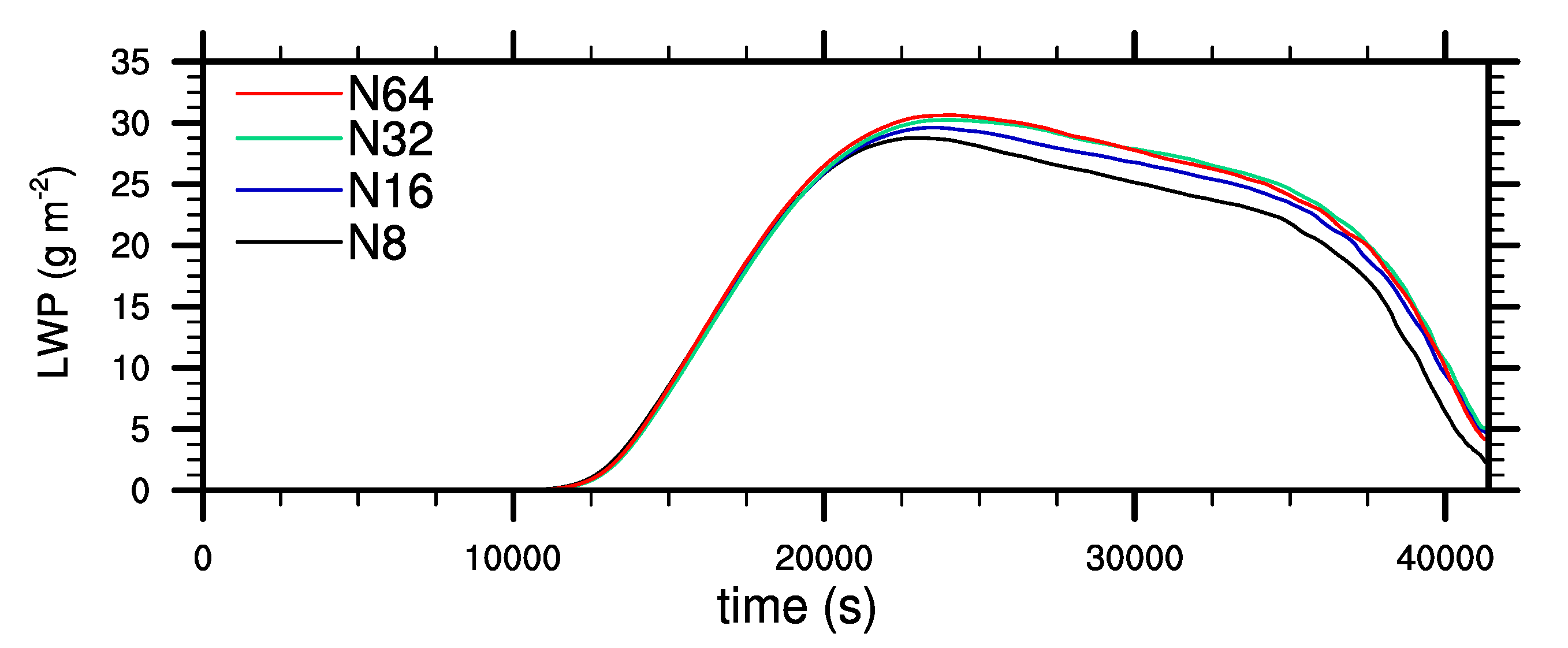
Appendix A. Sensitivity Study: Number of Superdroplets

We performed three-dimensional large-eddy simulations of a radiation fog event with different microphysics schemes. By using particle-based microphysics illustrated by explicit simulated Lagrangian particles, the general question arises how many of those particles are required for a convergent solution. Due to the extremely high computing time requirements of the simulations presented in the main part of this paper, some simplifications were made in the sensitivity studies. Mainly the curvature and solution effects of the aerosol were neglected, which leads to the elimination of the internal particle time step for the diffusional growth equation. Therefore, a comparatively large time step of 0.2 s could be used. The prescribed initial number concentration was set to 600 cm 3 . All other parameters were left constant. Four simulations were carried out with concentrations of 8, 16, 32 and 64 superdroplets per grid box. Figure A1 shows that the overall liquid water path is sensitive to the used number of superdroplets. However, increasing the superdroplet number leads to decreasing differences between the simulations. It can be seen that the results converge and satisfactory results are achieved with a superdroplet number of 32 particles per grid box. Deriving the superdroplet concentration to the physical space, yields concentrations of 0.5, 1, 2 and 4 superdroplets per cubic-meter. Compared to other studies using the LCM approach, this number is at the cutting-edge of current LCM applications [16,37].
Figure A1. Time series of liquid water path for the sensitivity studies with different superdroplet concentrations.
Atmosphere 11 00466 g0a1

References

  1. Gultepe, I.; Hansen, B.; Cober, S.; Pearson, G.; Milbrandt, J.; Platnick, S.; Taylor, P.; Gordon, M.; Oakley, J. The fog remote sensing and modeling field project. Bull. Am. Meteor. Soc. 2009, 90, 341–359. [Google Scholar] [CrossRef]
  2. Gultepe, I.; Tardif, R.; Michaelides, S.; Cermak, J.; Bott, A.; Bendix, J.; Müller, M.D.; Pagowski, M.; Hansen, B.; Ellrod, G.; et al. Fog research: A review of past achievements and future perspectives. Pure Appl. Geophys. 2007, 164, 1121–1159. [Google Scholar] [CrossRef]
  3. Price, J. Radiation fog. Part I: Observations of stability and drop size distributions. Bound.-Layer Meteorol. 2011, 139, 167–191. [Google Scholar] [CrossRef]
  4. Wilkinson, J.M.; Porson, A.N.; Bornemann, F.J.; Weeks, M.; Field, P.R.; Lock, A.P. Improved microphysical parametrization of drizzle and fog for operational forecasting using the Met Office Unified Model. Q. J. R. Meteorol. Soc. 2013, 139, 488–500. [Google Scholar] [CrossRef]
  5. Boutle, I.; Price, J.; Kudzotsa, I.; Kokkola, H.; Romakkaniemi, S. Aerosol-fog interaction and the transition to well-mixed radiation fog. Atmos. Chem. Phys. 2018, 18, 7827–7840. [Google Scholar] [CrossRef] [Green Version]
  6. Bott, A. On the influence of the physico-chemical properties of aerosols on the life cycle of radiation fogs. Bound.-Layer Meteorol. 1991, 56, 1–31. [Google Scholar] [CrossRef]
  7. Wendish, M.; Mertes, S.; Heintzenberg, J.; Wiedensohler, A.; Schell, D.; Wobrock, W.; Frank, G.; Martinsson, B.G.; Fuzzi, S.; Orsi, G.; et al. Drop size distribution and LWC in Po valley fog. Contrib. Atmos. Phys. 1998, 71, 87–100. [Google Scholar]
  8. Niu, S.; Liu, D.; Zhao, L.; Lu, C.; Lü, J.; Yang, J. Summary of a 4-year fog field study in northern Nanjing, Part 2: Fog microphysics. Pure Appl. Geophys. 2012, 169, 1137–1155. [Google Scholar] [CrossRef]
  9. Stolaki, S.; Haeffelin, M.; Lac, C.; Dupont, J.C.; Elias, T.; Masson, V. Influence of aerosols on the life cycle of a radiation fog event. A numerical and observational study. Atmos. Res. 2015, 151, 146–161. [Google Scholar] [CrossRef]
  10. Maalick, Z.; Kühn, T.; Korhonen, H.; Kokkola, H.; Laaksonen, A.; Romakkaniemi, S. Effect of aerosol concentration and absorbing aerosol on the radiation fog life cycle. Atmos. Environ. 2016, 133, 26–33. [Google Scholar] [CrossRef]
  11. Thies, B.; Egli, S.; Bendix, J. The Influence of Drop Size Distributions on the Relationship between Liquid Water Content and Radar Reflectivity in Radiation Fogs. Atmosphere 2017, 8, 142. [Google Scholar] [CrossRef] [Green Version]
  12. Mazoyer, M.; Burnet, F.; Denjean, C.; Roberts, G.C.; Haeffelin, M.; Dupont, J.C.; Elias, T. Experimental study of the aerosol impact on fog microphysics. Atmos. Chem. Phys. 2019, 19, 4323–4344. [Google Scholar] [CrossRef] [Green Version]
  13. Poku, C.; Ross, A.; Blyth, A.; Hill, A.; Price, J. How important are aerosol–fog interactions for the successful modelling of nocturnal radiation fog? Weather 2019, 74, 237–243. [Google Scholar] [CrossRef] [Green Version]
  14. Schwenkel, J.; Maronga, B. Large-eddy simulation of radiation fog with comprehensive two-moment bulk microphysics: Impact of different aerosol activation and condensation parameterizations. Atmos. Chem. Phys. 2019, 19, 7165–7181. [Google Scholar] [CrossRef] [Green Version]
  15. Köhler, H. The nucleus in and the growth of hygroscopic droplets. Trans. Faraday Soc. 1936, 32, 1152–1161. [Google Scholar] [CrossRef]
  16. Grabowski, W.W.; Morrison, H.; Shima, S.I.; Abade, G.C.; Dziekan, P.; Pawlowska, H. Modeling of Cloud Microphysics: Can We Do Better? Bull. Am. Meteorol. Soc. 2019, 100, 655–672. [Google Scholar] [CrossRef] [Green Version]
  17. Cohard, J.M.; Pinty, J.P.; Bedos, C. Extending Twomey’s analytical estimate of nucleated cloud droplet concentrations from CCN spectra. J. Atmos. Sci. 1998, 55, 3348–3357. [Google Scholar] [CrossRef]
  18. Khvorostyanov, V.I.; Curry, J.A. Aerosol size spectra and CCN activity spectra: Reconciling the lognormal, algebraic, and power laws. J. Geophys. Res. Atmos. 2006, 111. [Google Scholar] [CrossRef] [Green Version]
  19. Hoffmann, F.; Raasch, S.; Noh, Y. Entrainment of aerosols and their activation in a shallow cumulus cloud studied with a coupled LCM–LES approach. Atmos. Res. 2015, 156, 43–57. [Google Scholar] [CrossRef]
  20. Porson, A.; Price, J.; Lock, A.; Clark, P. Radiation fog. Part II: Large-eddy simulations in very stable conditions. Bound.-Layer Meteorol. 2011, 139, 193–224. [Google Scholar] [CrossRef]
  21. Maronga, B.; Bosveld, F. Key parameters for the life cycle of nocturnal radiation fog: A comprehensive large-eddy simulation study. Q. J. R. Meteorol. Soc. 2017, 143, 2463–2480. [Google Scholar] [CrossRef]
  22. Steeneveld, G.J.; de Bode, M. Unravelling the relative roles of physical processes in modelling the life cycle of a warm radiation fog. Q. J. R. Meteorol. Soc. 2018, 144, 1539–1554. [Google Scholar] [CrossRef]
  23. Tonttila, J.; Maalick, Z.; Raatikainen, T.; Kokkola, H.; Kühn, T.; Romakkaniemi, S. UCLALES–SALSA v1.0: A large-eddy model with interactive sectional microphysics for aerosol, clouds and precipitation. Geosci. Model Dev. 2017, 10, 169–188. [Google Scholar] [CrossRef] [Green Version]
  24. Maronga, B.; Gryschka, M.; Heinze, R.; Hoffmann, F.; Kanani-Sühring, F.; Keck, M.; Ketelsen, K.; Letzel, M.O.; Sühring, M.; Raasch, S. The Parallelized Large-Eddy Simulation Model (PALM) version 4.0 for atmospheric and oceanic flows: Model formulation, recent developments, and future perspectives. Geosci. Model Dev. 2015. [Google Scholar] [CrossRef] [Green Version]
  25. Maronga, B.; Banzhaf, S.; Burmeister, C.; Esch, T.; Forkel, R.; Fröhlich, D.; Fuka, V.; Gehrke, K.F.; Geletič, J.; Giersch, S.; et al. Overview of the PALM model system 6.0. Geosci. Model Dev. 2020, 13, 1335–1372. [Google Scholar] [CrossRef]
  26. Beare, R.J.; Macvean, M.K.; Holtslag, A.A.; Cuxart, J.; Esau, I.; Golaz, J.C.; Jimenez, M.A.; Khairoutdinov, M.; Kosovic, B.; Lewellen, D.; et al. An intercomparison of large-eddy simulations of the stable boundary layer. Bound.-Layer Meteorol. 2006, 118, 247–272. [Google Scholar] [CrossRef] [Green Version]
  27. Maronga, B.; Knigge, C.; Raasch, S. An Improved Surface Boundary Condition for Large-Eddy Simulations Based on Monin–Obukhov Similarity Theory: Evaluation and Consequences for Grid Convergence in Neutral and Stable Conditions. Bound.-Layer Meteorol. 2020, 174, 297–325. [Google Scholar] [CrossRef] [Green Version]
  28. Wicker, L.J.; Skamarock, W.C. Time-splitting methods for elastic models using forward time schemes. Mon. Weather Rev. 2002, 130, 2088–2097. [Google Scholar] [CrossRef]
  29. Williamson, J. Low-storage runge-kutta schemes. J. Comput. Phys. 1980, 35, 48–56. [Google Scholar] [CrossRef]
  30. Deardorff, J.W. Stratocumulus-capped mixed layers derived from a three-dimensional model. Bound.-Layer Meteorol. 1980, 18, 495–527. [Google Scholar] [CrossRef]
  31. Clough, S.A.; Shephard, M.W.; Mlawer, E.J.; Delamere, J.S.; Iacono, M.J.; Cady-Pereira, K.; Boukabara, S.; Brown, P.D. Atmospheric radiative transfer modeling: A summary of the AER codes, Short Communication. J. Quant. Spectrosc. Radiat. Transf. 2005, 91, 233–244. [Google Scholar] [CrossRef]
  32. Grabowski, W.W.; Dziekan, P.; Pawlowska, H. Lagrangian condensation microphysics with Twomey CCN activation. Geosci. Model Dev. 2018, 11, 103–120. [Google Scholar] [CrossRef] [Green Version]
  33. Rogers, R.R.; Baumgardner, D.; Ethier, S.A.; Carter, D.A.; Ecklund, W.L. Comparison of Raindrop Size Distributions Measured by Radar Wind Profiler and by Airplane. J. Appl. Meteorol. 1993, 32, 694–699. [Google Scholar] [CrossRef] [Green Version]
  34. Riechelmann, T.; Noh, Y.; Raasch, S. A new method for large-eddy simulations of clouds with Lagrangian droplets including the effects of turbulent collision. New J. Phys. 2012, 14, 065008. [Google Scholar] [CrossRef]
  35. Hoffmann, F. The effect of spurious cloud edge supersaturations in Lagrangian cloud models: An analytical and numerical study. Mon. Weather Rev. 2016, 144, 107–118. [Google Scholar] [CrossRef]
  36. Kogan, Y.L. The Simulation of a Convective Cloud in a 3-D Model With Explicit Microphysics. Part I: Model Description and Sensitivity Experiments. J. Atmos. Sci. 1991, 48, 1160–1189. [Google Scholar] [CrossRef] [Green Version]
  37. Hoffmann, F.; Noh, Y.; Raasch, S. The Route to Raindrop Formation in a Shallow Cumulus Cloud Simulated by a Lagrangian Cloud Model. J. Atmos. Sci. 2017, 74, 2125–2142. [Google Scholar] [CrossRef]
  38. Seifert, A.; Beheng, K.D. A double-moment parameterization for simulating autoconversion, accretion and selfcollection. Atmos. Res. 2001, 59, 265–281. [Google Scholar] [CrossRef]
  39. Seifert, A.; Beheng, K.D. A two-moment cloud microphysics parameterization for mixed-phase clouds. Part 1: Model description. Meteorol. Atmos. Phys. 2006, 92, 45–66. [Google Scholar] [CrossRef]
  40. Morrison, H.; Curry, J.A.; Shupe, M.D.; Zuidema, P. A New Double-Moment Microphysics Parameterization for Application in Cloud and Climate Models. Part II: Single-Column Modeling of Arctic Clouds. J. Atmos. Sci. 2005, 62, 1678–1693. [Google Scholar] [CrossRef] [Green Version]
  41. Ackerman, A.S.; VanZanten, M.C.; Stevens, B.; Savic-Jovcic, V.; Bretherton, C.S.; Chlond, A.; Golaz, J.C.; Jiang, H.; Khairoutdinov, M.; Krueger, S.K.; et al. Large-eddy simulations of a drizzling, stratocumulus-topped marine boundary layer. Mon. Weather Rev. 2009, 137, 1083–1110. [Google Scholar] [CrossRef] [Green Version]
  42. Geoffroy, O.; Brenguier, J.L.; Burnet, F. Parametric representation of the cloud droplet spectra for LES warm bulk microphysical schemes. Atmos. Chem. Phys. 2010, 10, 4835–4848. [Google Scholar] [CrossRef] [Green Version]
  43. Khairoutdinov, M.; Kogan, Y. A new cloud physics parameterization in a large-eddy simulation model of marine stratocumulus. Mon. Weather Rev. 2000, 128, 229–243. [Google Scholar] [CrossRef]
  44. Boers, R.; Baltink, H.K.; Hemink, H.; Bosveld, F.; Moerman, M. Ground-based observations and modeling of the visibility and radar reflectivity in a radiation fog layer. J. Atmos. Ocean Technol. 2013, 30, 288–300. [Google Scholar] [CrossRef]
  45. Jaenicke, R. Tropospheric Aerosols. In Aerosol-Cloud-Climate Interactions; Hobbs, P.V., Ed.; Academic Press: San Diego, CA, USA, 1993; pp. 1–31. [Google Scholar]
  46. Gultepe, I.; Müller, M.D.; Boybeyi, Z. A New Visibility Parameterization for Warm-Fog Applications in Numerical Weather Prediction Models. J. Appl. Meteorol. Climatol. 2006, 45, 1469–1480. [Google Scholar] [CrossRef]
  47. Hammer, E.; Gysel, M.; Roberts, G.C.; Elias, T.; Hofer, J.; Hoyle, C.R.; Bukowiecki, N.; Dupont, J.C.; Burnet, F.; Baltensperger, U.; et al. Size-dependent particle activation properties in fog during the ParisFog 2012/13 field campaign. Atmos. Chem. Phys. 2014, 14, 10517–10533. [Google Scholar] [CrossRef] [Green Version]
  48. Elias, T.; Dupont, J.C.; Hammer, E.; Hoyle, C.R.; Haeffelin, M.; Burnet, F.; Jolivet, D. Enhanced extinction of visible radiation due to hydrated aerosols in mist and fog. Atmos. Chem. Phys. 2015, 15, 6605–6623. [Google Scholar] [CrossRef] [Green Version]
  49. Zhang, X.; Musson-Genon, L.; Dupont, E.; Milliez, M.; Carissimo, B. On the influence of a simple microphysics parametrization on radiation fog modelling: A case study during parisfog. Bound.-Layer Meteorol. 2014, 151, 293–315. [Google Scholar] [CrossRef]
  50. Pilié, R.; Mack, E.; Kocmond, W.; Eadie, W.; Rogers, C. The life cycle of valley fog. Part II: Fog microphysics. J. Appl. Meteorol. 1975, 14, 364–374. [Google Scholar] [CrossRef] [Green Version]
Figure 1. Maritime and rural initial dry aerosol distributions for the LCM and BCM.
Atmosphere 11 00466 g001
Figure 2. Temporal evolution of liquid water path (a), droplet number concentration averaged over the fog layer (b), fog top height (c), visibility at 2 m height (d), sedimentation rate at the surface and surface (e) incoming longwave radiation (f). The vertical line and bars in (a) mark the time step and the range for the size distribution in Figure 4. The shaded areas in (d) shows the time frame where fog is present (applying the definition visibility < 1000 m) regarding LCM-M and LCM-R.
Atmosphere 11 00466 g002
Figure 3. Time-height cross-section of liquid water ratio (horizontally averaged) for rural (top panel) (a,b) and maritime (bottom panel) (e,f) aerosol conditions. In the left column results for LCM cases and on the right column for BCM cases are shown. Profiles on the right hand side display n c (c,g) and potential temperature θ (d,h) at the marked times (black vertical line in the cross-section). The shaded areas (c,g) show the liquid water mixing ratio as a qualitative measure. Here, areas of the same size represent equal values for q l .
Atmosphere 11 00466 g003
Figure 4. Instantaneous drop size distributions of number and mass density at 0300 UTC (a,b), 0600 UTC (c,d) and 0800 UTC (e,f) averaged over the fog layer of the simulations listed in Table 2. The shaded area indicates the shift of the spectrum in an interval of 1 h around the discrete value.
Atmosphere 11 00466 g004
Figure 5. Instantaneous drop size distributions at 0600 UTC at 2 m height of the simulations listed in Table 2. The shaded area indicates the shift of the spectrum in an interval of 1 h around the discrete value.
Atmosphere 11 00466 g005
Table 1. Aerosol size distributions for maritime and rural conditions after Jaenicke [45]. Here, the type defines the chemical species, i depicts the mode, n a , i is the number concentration of aerosol of that mode per cubic centimeter, r a , i is the dry aerosol radius in microns and  ln σ a , i is the logarithmic width of the distribution.
AerosolTypei n a , i (cm) 3 r a , i ( μ m) ln σ a , i
MaritimeNaCl11.33 × 10 2 0.00391.512
26.66 × 10 1 0.1330.484
33.06 × 10 0 0.290.912
RuralNH 4 NO 3 16.65 × 10 3 0.007390.518
21.47 × 10 2 0.02691.283
31.99 × 10 3 0.04190.612
Table 2. Overview of conducted simulations.
NameMicrophysical ModelAerosol
LCM-RLagrangian cloud modelrural
LCM-MLagrangian cloud modelmaritime
BCM-RBulk cloud modelrural
BCM-MBulk cloud modelmaritime

