Abstract
We present a mathematical model for the propagation of the shock waves that occur during planetary collisions. Such collisions are thought to occur during the formation of terrestrial planets, and they have the potential to erode the planet’s atmosphere. We show that, under certain assumptions, this evolution of the shock wave can be determined using the methodologies of Type II self similar solutions. In such solutions, the evolution of the shock wave is determined by boundary conditions at the shock front and a singular point in the shocked region. We show how the evolution can be determined for different equations of state, allowing these results to be readily used to calculate the atmospheric mass loss from planetary cores made of different materials. We demonstrate that, as a planetary shock converges to the self similar solution, it loses information about the collision that created it, including the impact angle for oblique collisions.
1. Introduction
The formation of terrestrial planets is thought to proceed in two phases. In the first phase, rocky cores form by accretion in the protoplanetary disc [1], and, in the second stage, multiple planetary cores merge to form planets after the disc evaporates [2,3]. Theoretical models predict that, when the disc evaporates, it will leave behind a large number of tightly packed planetary cores. Dynamical instabilities will excite eccentricities, which will cause the orbits to intersect and the cores to collide [4,5,6,7]. Among other things, these collisions can erode a planetary atmosphere.
It is difficult to observe planetary collisions directly, as they are expected, in the most optimistic scenario, to produce a faint, short (few hours) and hard (X-ray and EUV) transient [8]. Study of this phase is therefore based on theoretical or computational models, and indirect observational evidence, such as isotope ratios on Earth [9] or debris rings around exoplanetary systems [10]. Planetary collisions have been suggested as a possible mechanism to explain systems such as Kepler 107 [11], where a pair of neighbouring planets have very different average densities. Kepler 107b has a low density, indicating the presence of an atmosphere, while Kepler 107c, which is farther away from the host star, has a density almost three times larger than 107b, indicating a bare rocky core devoid of an atmosphere. If both planets started out with a thick atmosphere, other mechanisms, such as photoevaporation, could not have stripped Kepler 107c of its atmosphere while sparing 107b.
Simulations of giant collisions have been carried out by many authors in the past (e.g., [12]). However, these authors mostly considered the change in solid mass. For this purpose, the authors ran many simulations spanning a wide range of parameters. In contrast, for simulations of atmospheric mass loss due to giant collisions, most works have focused on a single specific case; e.g., Liu et al. [13] considered Kepler 36. A systematic study of atmospheric mass loss is carried out in [14,15], but only for head-on collisions. The model the authors developed considers two distinct shock waves. The first shock wave emerges from the impact site and propagates through the planet’s core. The first shock moves the ground, which produces another shock shock wave that travels through the atmospheric gas. Since the atmosphere has a declining density profile, the shock wave that travels through it accelerates as it moves up. At some point, the shock wave exceeds the escape velocity, and all the gas above this point is lost. For this reason, some of the gas column above the ground is expelled even if the ground move slower than the escape velocity.
Propagation of a shock due to an impact event has been studied using simulations [16,17] and experiments [18,19,20]. However, under certain assumptions, the shock can be described analytically, using the theory of self similar solutions [21]. The most famous solution of this kind is the Sedov Taylor solution for the strong adiabatic explosion [22,23]. In this case, the motion of the shock front is determined using conservation of energy. Such cases where the self similar motion can be determined using conservation laws are called Type I solutions. In contrast, the shock waves in planetary collisions are Type II solutions. In such cases, conservation laws cannot be used and the motion is determined by the behaviour near a singularity [24].
The intention of this paper is to explain how the evolution of the shock in the planet’s core can be described using the theory of self similarity. The structure of this paper is as follows. In Section 2, we describe the self similar solution of the shock propagating in the core. In Section 3, we demonstrate how the atmospheric mass loss can be estimated. Finally, we discuss the results in Section 4.
2. Core Shock
2.1. Impulsive Piston Problem
Let us consider an impact on a very large planet, so that the radius of curvature is unimportant and the ground can be considered flat. Such an impact will launch a shock wave that spreads as a hemisphere below the ground. When the radius of the shock wave is much larger than the size of the impactor, since there are no other length scales in this problem and the shock radius, R, grows as some power law in time . The purpose of this section is to estimate .
In general, modelling an oblique collision requires three spatial coordinates (e.g., radius measured from the impact site, angle from the normal to the surface from the impact site and an azimuthal angle around that normal). In the case of a head-on collision, we can use azimuthal symmetry to eliminate one spatial coordinate, but this leaves us with two spatial variables. It turns out that developing a self similar theory for even two spatial coordinates is quite challenging; thus, we turn to an even simpler problem—the impulsive piston problem [25,26]. In this case, we consider a slab symmetric, one-dimensional analogue to the self similar impact problem. In this scenario, a thin wafer hits a much thicker slab of material and both are perfectly cold prior to the collision. As a result of this collision, a shock wave emerges from the contact surface and travels into the target. Once the shock wave has travelled a distance much larger than the width of the wafer, there is no other relevant length scale in this process other than the position of the shock front, and hence we expect the shock wave to evolve in a self similar way.
A remarkable property of the impulsive piston problem is that the relation between the shock velocity and the swept up mass holds approximately also in the three-dimensional impact problem [15], i.e., a power law with the same exponent . In the remainder of this section, we present the mathematical formulation of the one-dimensional impulsive piston problem.
The impulsive piston problem was originally developed and solved in [25,27,28,29,30,31]. The authors reduced the hydrodynamic partial differential equations to ordinary differential equations, and used a multidimensional shooting method to determine . In contrast, the variables we chose allow us to reduce the problem to a single ordinary differential equation, but it comes at a cost. The cost is that we introduce a coordinate singularity, i.e., a place where the dimensional variables remain finite, but the dimensionless variables diverge. The price that we have to pay for this choice is that, for some range of values for the adiabatic index , the numerical integration is not continuous.
2.2. Self Similar Equations
The slab symmetric hydrodynamic equations in one dimension were given by Landau and Lifshitz [32], which are, respectively, the continuity, momentum and adiabatic energy equations, where is density, v is velocity, p is pressure and s is entropy:
We assume an ideal gas equation of state
where is the adiabatic index. Naturally, one would expect the material in a planetary core to have a more complicated equation of state. However, we argue that at very high pressures and temperatures all materials behave as ideal gases. This claim is based on the observation that in high pressure shock experiments many materials exhibit a linear relation between the shock velocity and the material velocity (e.g., [33,34]), as ideal gases would. Moreover, the effective adiabatic index can be inferred from the slope . We can replace the pressure by the sound speed using the relation of . After this substitution, we have a system of partial differential equations in . We make the assumption that the one-dimensional shock has a self similar behaviour, thus the position of the shock front evolves as a power law in time
where is a constant. One of the main goals of the analysis is determining . We can use the conservation of energy or momentum to obtain limits on this parameter: [26]. The partial differential equations can be reduced to ordinary differential equations in the dimensionless position . Following Landau and Lifshitz [32], we define dimensionless hydrodynamical variables in the following way:
After this substitution, the equations contain terms involving different time derivatives of X. These time derivatives can be factored out using Equation (5). In fact, these factors can be dealt with by just eliminating the second derivative using
where, according to Equation (5), we have . The parameter is the power law index of the shock velocity–position relation . The energy and momentum conservation limits on this parameter are . After making these adjustments and simplifying, the hydrodyna(mic equations) Equations (1)–(3) becomes the matrix equation where:
These equations are now linear in the derivatives , thus they can be isolated. Our choice of parameters allows us to go a step further and obtain a single ordinary differential equation involving just C and V. We note that
where
Dividing one equation by the other, we get a single ODE
where
and
2.3. Boundary Conditions
To integrate Equation (15), boundary conditions and the value of are needed. The boundary conditions at the shock front are given by the Rankine–Hugoniot conditions for a strong shock [26,32]
and
In some self similar problems, such as the Sedov Taylor explosion, the parameter can be inferred directly from conservation laws. Such problems are known as Type I solutions. In our case, however, is determined by the condition that the hydrodynamic trajectory passes smoothly through some singularity. These are called Type II solutions [24]. The singularity occurs at a point where information cannot propagate back to the shock front, and is therefore also referred to as the sonic point. Energy that flows through the sonic point cannot travel back to the shock front, and thus the energy available to sustain the shock is not conserved.
Equation (11) has a singularity when
This curve is known as the sonic line. On the sonic line, the denominator (Equation (17)) vanishes. To prevent a divergence, the numerator also has to vanish. This happens on a specific point on the sonic line, which we call the sonic point
and
Knowing the boundary conditions and , we can integrate from the sonic point to the shock front, as shown in Figure 1. The starting point is slightly shifted from the sonic point in the positive V direction by and in C direction by for some small . The slope at the sonic point is given by the equation:
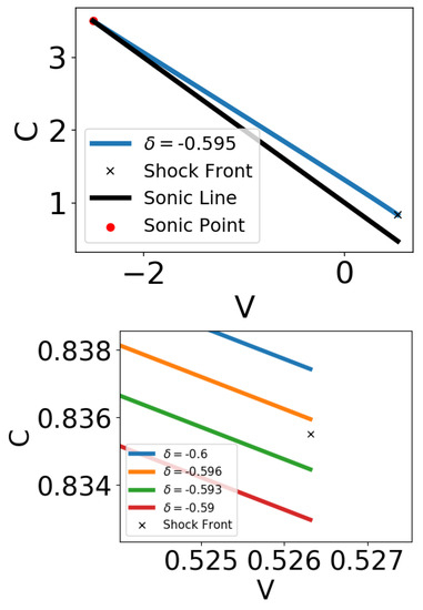
Figure 1.
Numerically integrated Hydrodynamic trajectories for , as an example for the general behaviour in the case , for various values of . The entire domain is shown in the top panel, and a zoomed in plot at shock front point is shown in the bottom panel. The integration proceeds continuously from the sonic point (red circle) to the shock front (black cross).
The correct value of is such that the curve satisfies both boundary conditions at the sonic point and the shock front. In practice, we use the shooting method to find the value of . We guess a value for , numerically integrate Equation (15) with respect to V from the sonic point to the shock front, and note the value of C at the shock front. We then use the bisection method to refine the value of to minimise the distance between the value of C obtained from numeric integration and its theoretical value (Equation (19)). An example for some hydrodynamic trajectories for the same value of but different values of can be seen in Figure 1, for .
In the case , numerical integration is straightforward since both the sonic point and the shock front are on the same side of the impact site (i.e., both when the impact site is ). The case is more complicated because the integration goes through . Because of the way we define the self similar variables (Equation (6)), they diverge at , even though the physical quantities v and c remain finite. We can circumvent this difficulty by noting that the Mach number, i.e., the ratio between the velocity and the speed of sound, remains finite and changes continuously across . The sonic point in the case lies in the fourth quadrant of the plane (i.e., positive V and negative C). Numerical integration proceeds to even higher values of V, moving away from the shock front. Far away from the sonic point, the curve attains some asymptotic slope, and this slope is the Mach number at , which we denote by . Once we have this piece of information, we can restart the numerical integration in the second quadrant (C is positive and V is negative), beginning from some arbitrarily highly negative (subscript r for restart) and . From this point, we can continue the numerical integration all the way to the shock front. An example for several hydrodynamic trajectories for (an important adiabatic index, corresponding to a diatomic ideal gas, for which the fluid dynamics equations can be solved analytically) can be seen in Figure 2.
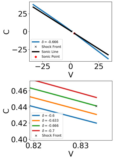
Figure 2.
Numerically integrated Hydrodynamic trajectories, integrated from the sonic point (red dot) to the shock front (black cross) for , as an example for the case , for different values of . The entire domain is shown in the top panel, and a zoomed in plot at shock front point is shown in the bottom panel. The integration goes from the sonic point in the fourth quadrant and proceeds down and to the right. After passing through the integration reappears in the second quadrant (top left corner) and travels to the shock front point.
Thus, for every value of , we can obtain the corresponding value of . The relation between them is shown in Figure 3. These results are consistent with a previous work [25]. We note that, in the limit , we get , which corresponds to momentum conservation. However, in the limit , the solution does not converge to , which corresponds to energy conservation, but to a different value. This is discussed in more details in the next section.
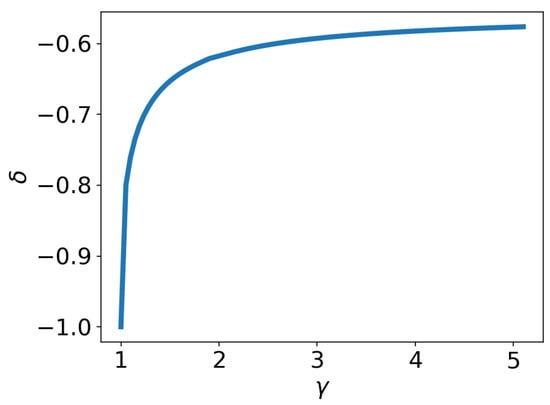
Figure 3.
Shock deceleration parameter as a function of the adiabatic index for the impulsive piston problem. Values are compatible with those of Adamskii and Popov [25], as well as those in Table 12.2 of [26].
2.4. Comparison with Experiments
We note that the results obtained in this section are in accord with the numerical simulations presented in [15], which found that, for the three-dimensional impact problem, the shock decelerates roughly as (where m is the swept up mass) for (corresponding to a monatomic ideal gas), where the model presented here predicts . The model here also explains impact experiments, although the translation between the theoretical results and the experimental results is not straightforward. In experiments, such as those described in [35], a projectile is fired at a slab of some material and the radius of the resulting crater is measured. In materials without shear strength, such as fluids, the crater basin stops growing when the pressure inside the crater is comparable to the hydrostatic pressure. The analysis above gives us a relation between the shock velocity and the swept up mass , where m is the swept up mass, and in a three-dimensional case it scales as a cube of the radius , where, for simplicity, is the initial mass density of both projectile and target. If we denote the radius of the projectile by a and we assume that the shock sweeps a mass comparable to the projectile before decelerating, then the relation between the shock velocity and the crater radius is roughly given by
where U is the initial projectile velocity. The pressure inside the crater is roughly given by , while the hydrostatic pressure is given by , where g is the gravitational acceleration. Equating the two pressures yields a relation between the volume of the crater (where is the terminal size of the crater) and the properties of the projectile
where we define the same dimensionless variables , as in [35]. We note that the scaling laws found above are consistent with those obtained in [36]. To produce a prediction, we need to estimate the effective adiabatic index. This can be done in different kinds of high pressure experiments, where a material is shocked and the material and shock velocity are measured. At high velocities, the ratio between the two tends to a constant, , and for an ideal gas , thus . For water, equation of state experiments yield [37], thus the effective adiabatic index our model yields and . The value obtained from experiments in water is [35]. Overall, despite our crude approximations, we obtain a value relatively close to the experimental value.
2.5. Asymptotic Case
In this section, we consider the case . This corresponds to a very stiff equation of state, such as that of a metal. For this reason, it might be useful in modelling shocks planets with a high metal content like the planet Mercury. The limit was considered by Adamskii and Popov [25], but obtained with a slightly different framework. In this case, we cannot use the equations developed above. Part of the reason is that the integration domain shrinks to zero width in this limit. To overcome this difficulty, we define a new variable . In this new variable, the integration domain becomes , and thus remains finite in the limit . The expression for the derivative in the new variable is given by
At the sonic point, the slope is given by
We can determine using the shooting method described in the previous section. This case is actually simpler, because it does not depend on , thus at the sonic point and at the shock front. A few hydrodynamic trajectories for different values of are shown in Figure 4. Using numerical root finding methods, we find that , in accordance with Adamskii and Popov [25]. Interestingly, this result is different from the energy conservation limit .
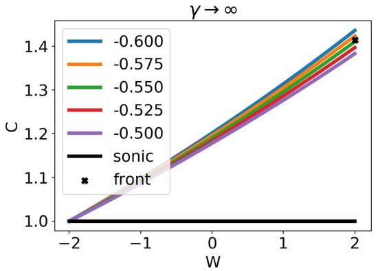
Figure 4.
Hydrodynamic trajectories for the case . Different coloured lined represent trajectories with different values of . The sonic line is represented by the black line, and the shock front by the black cross.
2.6. Analytic Case
For most values of , numerical integration has to be performed to obtain the power law index . However, for (corresponding to a diatomic ideal gas), it is possible to obtain a completely analytic solution, and the shooting method is not required [25]. Here we briefly describe the analytic solution and the hydrodynamic profiles in the case . The dimensionless hydrodynamic quantities in terms of , obtained from Adamskii and Popov [25], are
We can see that, at the shock front, where , the dimensionless velocity and speed of sound are , , as verified by the coordinates of the black X in the second graph of Figure 2. We also note that diverge as . From the shooting method, we obtain , which is consistent with the results in Figure 2. The velocity, density and pressure profiles, normalized to their respective quantities at the shock front, are shown in Figure 5.
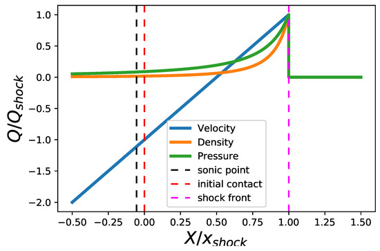
Figure 5.
Normalized velocity, density and pressure around the shock region. The shock front, sonic point and initial contact location are labelled.
We note that due to a fortunate coincidence, silica under high pressure behaves as an ideal gas with an adiabatic index [15]. Silica makes up most of the mass in the Earth and other terrestrial planets, and, therefore, this solution turns out to be extremely useful in describing shock waves in planetary collisions.
3. Atmospheric Mass Loss
In this section, we demonstrate how the atmospheric mass loss from a giant collision is estimated. The dependence of the mass loss on impactor size and velocity in head-on collisions was studied by Yalinewich and Schlichting [15]; thus, in this section, we consider the effects of obliquity. For this purpose, we ran simulations of collisions between planetary cores and planets. These simulations were run using the moving mesh numerical simulation RICH [38]. We use an ideal gas equation of state with an adiabatic index . The planet and planetary core are described as blobs with uniform density. Since the simulation cannot handle actual vacuum, we fill the computational domain with a very tenuous gas, whose density is lower than that of the planet by a factor of . We do not include gravity, because it invalidates the self similar solution, leading to a much more difficult problem to solve. In addition, in high velocity impacts (such as the simulations run here), excluding gravity does not result in a significant difference. The entire domain has an initially uniform pressure such that the speed of sound in the planet is of the impact velocity. Lastly, to simplify the calculation, we performed these simulations in a 2D Cartesian geometry. This means that the planet and planetary cores are not represented by spheres, but by cylinders. This detail greatly simplifies the calculation, but at the cost of introducing deviations from the real problem. However, as discussed in the previous section, the self similar solution in Lagrangian coordinates is approximately maintained in different geometries. This means that, so long as we are using the appropriate quantities, the results should not differ considerably from the spherical problem. The main difference between the cylindrical and spherical collisions is the relation between the swept up mass and the shock radius. In both cases, the mass is zero when the shock radius is zero, and equal to the target mass when the shock radius is twice the target radius. In the spherical case, however, the swept up mass always exceeds that of the cylindrical case at the same radius, thus we expect the atmospheric mass in the cylindrical case to over estimate that in the spherical case.
Figure 6 shows four log density snapshots from an oblique collision, where the radius of the impactor is times the radius of the planet. The figure shows a shock wave emanating from the impact site that travels through the planet, and obliterates it, since there is not gravity to hold it together.
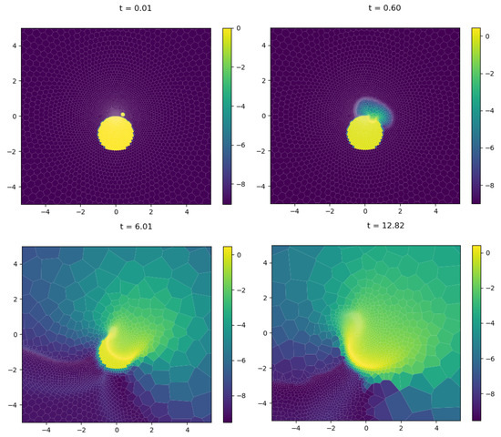
Figure 6.
Snapshots from a simulation at different times of a collision between a planet and a planetary core whose radius is a factor of smaller. We do not include gravity, thus the planet is obliterated in the end. The simulation is performed using a moving mesh hydrodynamic simulation, thus the polygons are actual computational cells.
One of the predictions of self similar theory is the loss of information about the initial conditions. Alternatively, different initial conditions lead to the same solution. To demonstrate this effect, in Figure 7 we plotted the ground velocities at different latitudes, measured from the impact site for an impactor whose radius is 0.01 of the target radius, for different impact factors. If we normalise the velocity according to the normal component of the velocity, all profiles become very similar to one another, thus demonstrating the loss of information about the details of the collision.
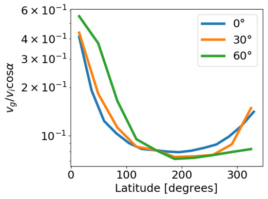
Figure 7.
Ground velocity ratio (ground velocity divided by the normal of impactor velocity) from the shock as a function of the position of the planet, for three different colliding angles. The ratio between the impactor and target radii is 0.01. The fact these curves are similar to one another demonstrates that in the self similar shocks lose some of the information about the initial conditions.
As the shock moves through the planet, it moves the ground, which pushes against the atmospheric gas column above it. In this sense, the ground acts as a piston, which sends a shock that moves up and away from the ground, accelerating due to the declining atmospheric mass density. The mass loss from each gas column as a function of ground velocity was worked out by Schlichting et al. [14]. By integrating the local atmospheric loss across the entire surface, we can obtain the total atmospheric mass loss. By running the simulation with different impact parameter (or offset) and different impactor to target radius ratios (but fixed velocity, which we set to be 1.5 times the escape velocity), we obtain a map of atmospheric mass loss shown in Figure 8. One of the interesting features of this map is that, for small impactors, the offset has very little influence on the outcome. This is because small enough impactors deposit all their energy in the target regardless of obliquity. This trend is in agreement with the findings of Yalinewich and Schlichting [15], who showed that, when the shock radius is considerably larger than the size of the impactor, the shock wave tends to the self similar solution found in the previous section, and in the process loses some of the information about the initial conditions (i.e., fast and small impactors create the same shock wave as slow and big impactors). The loss of information about the initial conditions is a common consequence of self similar solution [21].
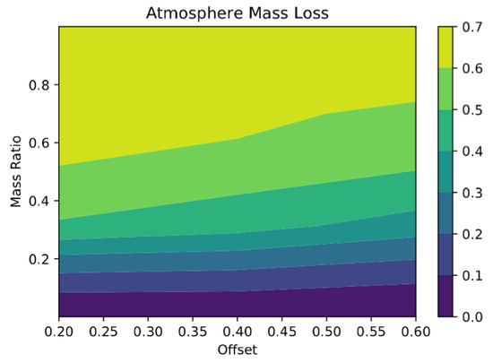
Figure 8.
A map of the atmospheric mass loss as a function of the mass ratio between the impactor and target, and the offset between the centres normal to the initial velocity difference, or impact parameter. The velocity is held fixed at 1.5 times the escape velocity.
4. Conclusions
Planet formation involves a phase of giant collisions, when planets and planetary cores smash into each other. These collisions erode the planet’s atmosphere. A key ingredient in modelling this mass loss is the evolution of the resulting shock wave in the core of the planet.
To justify the use of self similar solutions, we had to make a number of simplifying assumptions. First, we had to neglect all dimensional parameters in the problem; thus, such solutions only apply for shock radii much larger than the impactor on the one hand, but much smaller than the planet on the other hand. Second, we had to assume a strong shock, so that the impact velocity has to be much larger than the escape velocity. Third, we used an ideal gas equation of state, whereas real materials have a more complicated equation of state, which includes phase transitions. We argue that, at high pressures and velocities, all materials behave as ideal gases. Moreover, high pressure experiments can be used to determine the effective adiabatic index for different materials [15]. These assumptions are justified for high velocity collisions. Such collisions are likely to happen when the Keplerian orbital velocity is larger than the escape velocity from the planet, as is the case for close in terrestrial planets.
Even with all these assumptions, the problem is still too complicated to be solved analytically; thus, we simplified it even further by considering the one-dimensional analogue—the impulsive piston problem. This problem is a Type II self similar shocks, where the evolution of the shock wave is not determined by some conservation law, but according to a singularity behind the shock front. By requiring that the hydrodynamic profiles satisfy both conditions at the shock front and the singularity, we can obtain , where is the shock velocity and m is the swept up mass. It turns out that this relation holds approximately even in different geometries, i.e., in the three-dimensional impact.
It is surprising that, despite the many simplifying assumptions made here, the amounts of atmospheric mass loss predicted from this model is similar to more complicated models, which take into account all the effects considered here [15]. In the future, it would be interesting to see if this model can be refined to include some of the effects previously neglected.
Author Contributions
A.Y. drafted the manuscript and oversaw the analytic and numerical calculations. A.R. carried out the analytic and numeric calculation and took part in writing the manuscript. All authors have read and agreed to the published version of the manuscript.
Funding
This research received no external funding.
Acknowledgments
A.Y. would like to thank Hilke Schlichting and Re’em Sari for the useful discussions. A.Y. is supported by the Vincent and Beatrice Tremaine Fellowship. This work made use of the sympy [39], numpy [40] and matplotlib [41] Python packages.
Conflicts of Interest
The authors declare no conflict of interest.
References
- Armitage, P.J. A Brief Overview of Planet Formation; Springer: Berlin, Germany, 2018; p. 135. [Google Scholar] [CrossRef]
- Agnor, C.B.; Canup, R.M.; Levison, H.F. On the Character and Consequences of Large Impacts in the Late Stage of Terrestrial Planet Formation. Icarus 1999, 142, 219–237. [Google Scholar] [CrossRef]
- Chambers, J.E. Making More Terrestrial Planets. Icarus 2001, 152, 205–224. [Google Scholar] [CrossRef]
- Chambers, J.; Wetherill, G.; Boss, A. The Stability of Multi-Planet Systems. Icarus 1996, 119, 261–268. [Google Scholar] [CrossRef]
- Zhou, J.L.; Lin, D.N.C.; Sun, Y.S. Post-Oligarchic Evolution of Protoplanetary Embryos and the Stability of Planetary Systems. Astrophys. J. 2007, 666, 423–435. [Google Scholar] [CrossRef]
- Obertas, A.; Van Laerhoven, C.; Tamayo, D. The stability of tightly-packed, evenly-spaced systems of Earth-mass planets orbiting a Sun-like star. Icarus 2017, 293, 52–58. [Google Scholar] [CrossRef]
- Rice, D.R.; Rasio, F.A.; Steffen, J.H. Survival of non-coplanar, closely-packed planetary systems after a close encounter. MNRAS 2018, 481, 2205–2212. [Google Scholar] [CrossRef]
- Zhang, B.; Sigurdsson, S. Electromagnetic Signals from Planetary Collisions. Astrophys. J. 2003, 596, L95–L98. [Google Scholar] [CrossRef]
- Schlichting, H.E.; Mukhopadhyay, S. Atmosphere Impact Losses. Space Sci. Rev. 2018, 214, 34. [Google Scholar] [CrossRef]
- Thompson, M.A.; Weinberger, A.J.; Keller, L.; Arnold, J.A.; Stark, C. Studying the Evolution of Warm Dust Encircling BD +20 307 Using SOFIA. Astrophys. J. 2019, 875, 45. [Google Scholar] [CrossRef]
- Bonomo, A.S.; Zeng, L.; Damasso, M.; Leinhardt, Z.M.; Justesen, A.B.; Lopez, E.; Lund, M.N.; Malavolta, L.; Aguirre, V.S.; Buchhave, L.A.; et al. A giant impact as the likely origin of different twins in the Kepler-107 exoplanet system. Nat. Astron. 2019, 3, 416–423. [Google Scholar] [CrossRef]
- Stewart, S.T.; Leinhardt, Z.M. Collisions between Gravity-Dominated Bodies: 2. The Diversity of Impact Outcomes during the End Stage of Planet Formation. Astrophys. J. 2011, 745, 79. [Google Scholar] [CrossRef]
- Liu, S.F.; Hori, Y.; Lin, D.N.; Asphaug, E. Giant impact: an efficient mechanism for the devolatilization of super-earths. Astrophys. J. 2015, 812, 164. [Google Scholar] [CrossRef]
- Schlichting, H.; Sari, R.; Yalinewich, A. Atmospheric mass loss during planet formation: The importance of planetesimal impacts. Icarus 2015, 247, 81–94. [Google Scholar] [CrossRef]
- Yalinewich, A.; Schlichting, H.E. Atmospheric Mass Loss from High Velocity Giant Impacts. Mon. Not. R. Astron. Soc. 2018, 486, 2780–2789. [Google Scholar] [CrossRef]
- Potter, R.; Collins, G.; Kiefer, W.; McGovern, P.; Kring, D. Constraining the size of the South Pole-Aitken basin impact. Icarus 2012, 220, 730–743. [Google Scholar] [CrossRef]
- Monteux, J.; Arkani-Hamed, J. Shock wave propagation in layered planetary interiors: Revisited. Icarus 2019, 331, 238–256. [Google Scholar] [CrossRef]
- Holsapple, K.A.; Housen, K.R. Momentum transfer in asteroid impacts. I. Theory and scaling. Icarus 2012, 221, 875–887. [Google Scholar] [CrossRef]
- Mazzariol, L.M.; Alves, M. Experimental verification of similarity laws for impacted structures made of different materials. Int. J. Impact Eng. 2019, 133, 103364. [Google Scholar] [CrossRef]
- Holsapple, K.A. The scaling of impact phenomena. Int. J. Impact Eng. 1987, 5, 343–355. [Google Scholar] [CrossRef]
- Barenblatt, G.I. Scaling, Self-similarity, and Intermediate Asymptotics; Cambridge University Press: Cambridge, UK, 1996. [Google Scholar] [CrossRef]
- Sedov, L.I. Propagation of strong blast waves. Prikl. Mat. Mekh 1946, 10, 241–250. [Google Scholar]
- Taylor, G.I. The formation of a blast wave by a very intense explosion I. Theoretical discussion. Proc. R. Soc. Lond. A 1950, 201, 159–174. [Google Scholar]
- Waxman, E.; Shvarts, D. Second-type self-similar solutions to the strong explosion problem. Phys. Fluids A Fluid Dyn. 1993, 5, 1035–1046. [Google Scholar] [CrossRef]
- Adamskii, V.B.; Popov, N.A. The motion of a gas under the action of a pressure on a piston, varying according to a power law. J. Appl. Math. Mech. 1959, 23, 793–806. [Google Scholar] [CrossRef]
- Zel’dovich, Y.B.; Raizer, Y.P.; Zel’dovich, Y.B.; Raizer, Y.P. Physics of Shock Waves and High-Temperature Hydrodynamic Phenomena; Academic Press: New York, NY, USA, 1967. [Google Scholar]
- Hafele, W. Zur analytischen Behandlung ebener, starker, instationärer Stoßwellen. Z. Nat. Sect. A J. Phys. Sci. 1955, 10, 1006–1016. [Google Scholar] [CrossRef][Green Version]
- Hoerner, S.V. Lösungen der hydrodynamischen Gleichungen mit linearem Verlauf der Geschindigkeit. Z. Nat. Sect. A J. Phys. Sci. 1955, 10, 687–692. [Google Scholar] [CrossRef]
- Adamskii, V.B. Integration of a system of autosimulating equations for the problem of a short duration shock in a cold gas. Sov. Phys. Acoust. 1956, 2, 3–9. [Google Scholar]
- Zhukov, A.I.; Kazhdan, Y.M. The motion of a gas under the action of a short-lived impulse. Akust. Zhur 1956, 2, 352–357. [Google Scholar]
- Zeldovich, Y.B. The motion of a gas under the action of a short lived pressure. Akust. Zhur 1956, 2, 28–38. [Google Scholar]
- Landau, L.D.; Lifshitz, E.M. Fluid Mechanics; Pergamon Press: Oxford, UK, 1987. [Google Scholar] [CrossRef]
- McCoy, C.A.; Gregor, M.C.; Polsin, D.N.; Fratanduono, D.E.; Celliers, P.M.; Boehly, T.R.; Meyerhofer, D.D. Shock-wave equation-of-state measurements in fused silica up to 1600 GPa. J. Appl. Phys. 2016, 119, 215901. [Google Scholar] [CrossRef]
- Dattelbaum, D.; Coe, J. Shock-Driven Decomposition of Polymers and Polymeric Foams. Polymers 2019, 11, 493. [Google Scholar] [CrossRef]
- Holsapple, K.A.; Holsapple, A.K. The Scaling of Impact Processes in Planetary Sciences. Annu. Rev. Earth Planet. Sci. 1993, 21, 333–373. [Google Scholar] [CrossRef]
- Housen, K.R.; Schmidt, R.M.; Holsapple, K.A. Crater ejecta scaling laws: Fundamental forms based on dimensional analysis. J. Geophys. Res. 1983, 88, 2485. [Google Scholar] [CrossRef]
- Gojani, A.B.; Ohtani, K.; Takayama, K.; Hosseini, S.H.R. Shock Hugoniot and equations of states of water, castor oil, and aqueous solutions of sodium chloride, sucrose and gelatin. Shock Waves 2016, 26, 63–68. [Google Scholar] [CrossRef]
- Yalinewich, A.; Steinberg, E.; Sari, R. Rich: Open-source hydrodynamic simulation on a moving Voronoi mesh. Astrophys. J. Suppl. Ser. 2015, 216. [Google Scholar] [CrossRef]
- Meurer, A.; Smith, C.P.; Paprocki, M.; Čertík, O.; Kirpichev, S.B.; Rocklin, M.; Kumar, A.; Ivanov, S.; Moore, J.K.; Singh, S.; et al. SymPy: symbolic computing in Python. PeerJ Comput. Sci. 2017, 3, e103. [Google Scholar] [CrossRef]
- Oliphant, T.E. A Guide to NumPy; Trelgol Publishing: Scotts Valley, CA, USA, 2006; Volume 1. [Google Scholar]
- Hunter, J.D. Matplotlib: A 2D graphics environment. Comput. Sci. Eng. 2007, 9, 90–95. [Google Scholar] [CrossRef]
© 2020 by the authors. Licensee MDPI, Basel, Switzerland. This article is an open access article distributed under the terms and conditions of the Creative Commons Attribution (CC BY) license (http://creativecommons.org/licenses/by/4.0/).