Measurement and Prediction of Wind Fields at an Offshore Site by Scanning Doppler LiDAR and WRF

Abstract

LiDAR-based wind speed measurements have seen a significant increase in interest in wind energy. However, reconstruction of wind speed vector from a LiDAR-measured radial wind speed is still a challenge. Furthermore, for extensive application of LiDAR technology, it can be used as a means to validate simulation and analytical models. To that end, this study employed scanning Doppler LiDAR for assessment of wind fields at an offshore site and compared Weather Research and Forecasting (WRF)-based mesoscale simulations and several wake models with the measurements. Firstly, the effect of carrier-to-noise-ratio (CNR) and data availability on the quality of scanning LiDAR measurements was evaluated. Analysis of vertical profiles show that the average wind speed is higher for wind blowing from the sea than that blowing from the land. Furthermore, profiles obtained from the WRF simulation also show a similar tendency in the LiDAR measurements in general, though it overestimates the wind speeds at higher altitudes. A method for reconstruction of wind fields from plan-position indicator (PPI) and range height indicator (RHI) scans of LiDAR-measured line of sight velocities was then proposed and first used to investigate the effect of coastal terrain. An internal boundary layer with strong shear could be observed to develop from the coastline. Finally, the flow field around wind turbine was measured using PPI scan and used to validate wake models.

1. Introduction

Measurement and collection of accurate wind data is important for a range of wind energy applications, including wind resource evaluation for prospective wind farm sites, optimization of farm layouts, and control of turbines. The general practice in the wind energy industry is to use instruments mounted at a single height or at multiple heights on meteorological towers in order to collect wind data. However, due to structural and cost constraints, such towers are usually about 50 m to 100 m in height; thus, they cannot measure the wind field across the rotor of recent utility-scale turbines with typical hub heights of 100 to 130 m and rotor diameters of 150 to 200 m. As a result, remote sensing techniques and in particular LiDAR technologies are getting increasingly popular in wind energy research due to their ability to measure wind speeds over large regions and higher altitudes. Another crucial advantage of LiDARs over conventional meteorological masts is that the former provides flexibility regarding transportation and installation. This can be particularly important for offshore sites, where installation of a meteorological tower with either a fixed or floating platform can be prohibitively expensive.

Doppler LiDAR measures wind speed by emitting a laser beam that gets Doppler-shifted after being backscattered from aerosol particles, which are assumed to be moving at the same speed as the wind. This Doppler shift is used to compute the wind speed along the beam direction, which is known as the line of sight (LOS) velocity or radial velocity ($u_r$). Various methods have been proposed for the retrieval of the velocity vector from LiDAR-measured LOS velocity. Two approaches which have found widespread use in the retrieval of vertical profiles of wind speed are velocity azimuth display (VAD) and Doppler beam swinging (DBS). The VAD method employs a complete conical scan to collect closely spaced radial wind speed data [1]. The vertical profile of the wind speed are then deduced by fitting the $u_r$ at each height to the Fourier series using statistical methods, such as least-square analysis [2,3]. Unlike VAD, the DBS method only requires 4 or 5 beams to analytically deduce the wind speed at each height (cf. Section 2.2).

An increasing number of studies have been conducting measurement campaigns to verify LiDAR measurements against tower-mounted cup or sonic anemometers or to compare mean wind speeds measured using different types of LiDARs. Smith et al. evaluated a scanning Doppler LiDAR positioned adjacent to a met mast with calibrated anemometers [4]. They reported excellent correlation between the LiDAR and cup anemometers with a coefficient of determination ($R^2$) of 0.98 at 100m height. In a measurement campaign by Lang and McKeogh [5], at a complex terrain, they showed that both the slope and $R^2$ for a LiDAR-cup anemometer comparison was approximately 0.97 at a height of 100 m. Goit et al. investigated the accuracy of LiDAR by comparing long-term wind data against the tower mounted anemometers, and further evaluated the power and load distributions for the NREL 5-MW wind turbine obtained from the LiDAR-measured wind speeds [6]. Several other studies have also conducted similar inter-comparisons between LiDAR-measured wind speeds and wind speeds measured by tower-mounted anemometers (see, e.g., Ref. [7,8,9]). However, most of the validation studies were conducted for the altitudes lower than 150 m, and none of these studies investigated the effect of data availability. This indicates that the quality of measurements for several availability limits and for several carrier-to-noise-ratio (CNR) threshold values need to be investigated further.

Both DBS and VAD techniques have limitations in that they cannot account for horizontal variations and are therefore unable to generate velocity fields from the volume scan. To address this issue, Easterbook [10] and Waldteufel and Corbin [11] proposed the velocity volume processing (VVP) method, in which volumetric scan data is divided into several small analysis volumes, and the mean wind speed for each volume is estimated using multivariate regression analysis. This method assumes that the actual wind field is spatially linear and time invariant (see Ref. [3,12] for details). However, the method strongly depends on the size of the analysis volume and the number of measured $u_r$ data points in the volume. This will result in a very coarse resolution of the retrieved wind field in the region further away from the LiDAR. Therefore, the method is not popular in wind energy applications. A practical approach which is more common in wind energy is to perform scans along the mean wind direction, so that no further processing is required [13,14]. This method, however, has not been validated and it cannot be applied to sites where the wind direction changes with time. In the current study, a variation of this approach is employed where the velocity field is computed from the combination of LiDAR-measured LOS velocities and wind directions measured by a wind vane mounted on a meteorological tower (or a turbine nacelle). It should be noted that multiple studies have employed dual and triple LiDARs to collect more accurate wind speed data [15,16]. However, deploying two or three LiDARs can significantly increase the cost.

The objective of this study was to evaluate the performance of scanning Doppler LiDAR technology in the measurement of wind profiles and to propose a method for the reconstruction of wind fields from LiDAR-measured LOS velocity data. The LiDAR measurement data was further used to observe the near-shore marine atmospheric boundary layer (ABL) by comparing the wind blowing from the land and that from the sea and by considering the effect of coastal terrain. Furthermore, LiDAR measurement data was used to validate numerical simulations conducted using a mesoscale model. Finally, the flow field around the wind turbine was measured and analyzed to investigate the wake characteristics. The measurement data was also used to validate several wake models.

2. Measurement and Prediction Methods

This section first describes the test facility and the measurement devices. This is followed by discussions about three scan modes and the methods for the retrieval of velocity vectors from LOS velocity data. Finally, the details about the WRF (Weather Research and Forecasting) for the wind field prediction of the site is presented.

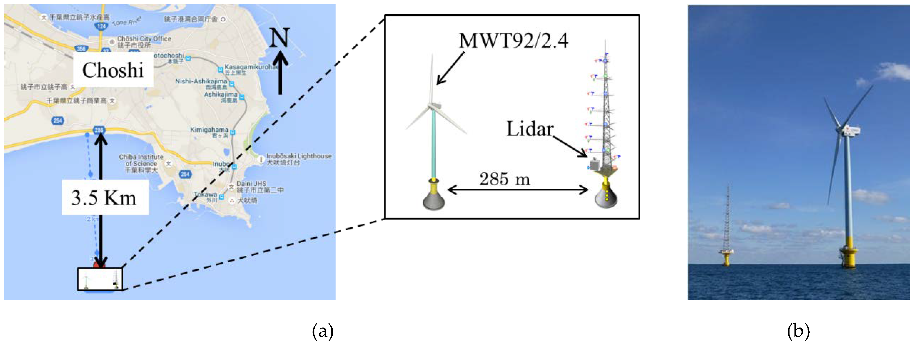
2.1. Test Site for Wind Field Measurement and Prediction

The measurements were collected from the Choshi offshore wind energy test facility located about 3.5 Km offshore of Choshi city of Chiba prefecture, Japan. As shown in Figure 1, the facility consists of a 2.4 MW wind turbine (MWT92/2.4) with a rotor diameter $\mathrm{D}=92$ m and a hub height $z_{\mathrm{h}}=80$ m, and a meteorological tower located 285 m east from the turbine. The meteorological tower has a height of 95 m, with 3D sonic anemometers (SAT-600A of Sonic Corporation) located at $40\mathrm{m},60\mathrm{m},\mathrm{and}80\mathrm{m}$. In addition to this, cup anemometers and wind vanes are installed between heights 20 m and 90 m at an interval of 10 m. The tower has a platform at a height of 15 m above the mean sea level. Two LiDARs, WindCube V1 (Leosphere, Orsay, France) and a scanning Doppler LiDAR (WindCube100S), are mounted on this platform. V1 is a profiling LiDAR; therefore, it can only measure vertical profiles at the installation point. WindCube 100S is capable of performing 3D volumetric scans [17]. Except for the validation purpose, the current study primarily used WindCube100S. Note that measurements from the V1 LiDAR were already validated against measurements from a sonic anemometer [18].

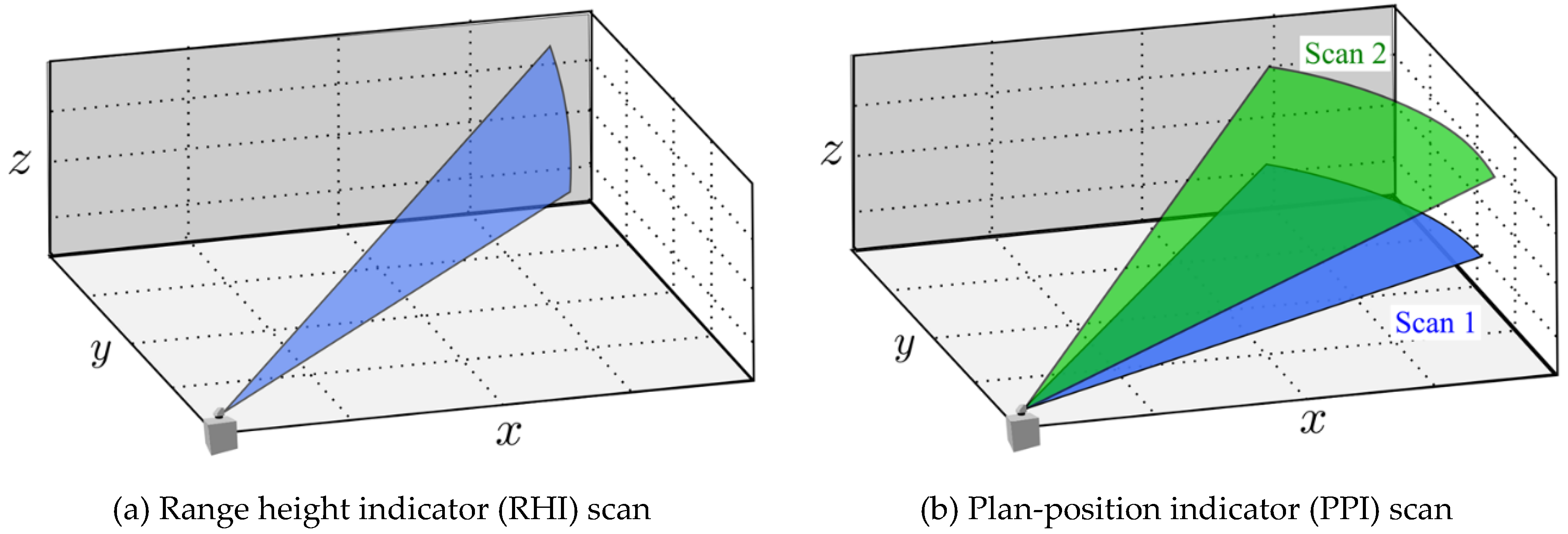
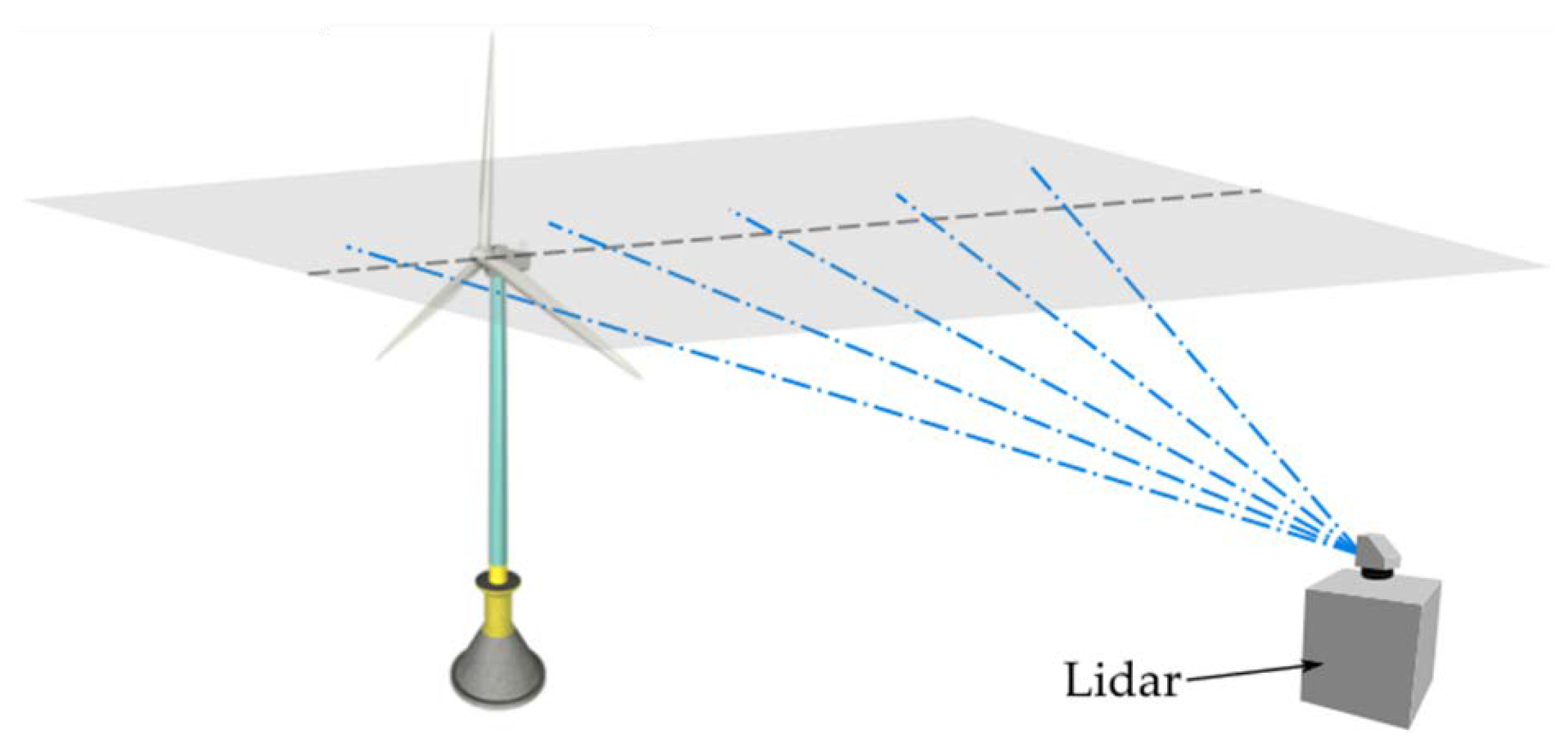
2.2. Wind Field Measurement by Scanning Doppler LiDAR

In order to retrieve vertical profiles of wind speeds and directions, line-of-site (LOS) wind speeds ($u_r$) were measured in the Doppler Beam Swinging (DBS) scanning configuration, shown schematically in Figure 2. In this configuration, the LiDAR beam is swung from north to east to south to west and to vertical directions. The wind speed can then be calculated at each measurement height using:

$$\begin{gathered} u=\frac{u_{rE}-u_{rW}}{2\cos \varphi } \\ v=\frac{u_{rN}-u_{rS}}{2\cos \varphi } \\ w=u_{rV}, \end{gathered}$$

(1)

where $u, v, w$ are wind speed components in west to east, north to south, and vertical directions, respectively. $u_{rE}, u_{rW}, u_{rN}, u_{rS},u_{rV}$ are radial wind speeds along the LOS measured in east, west, north, south, and vertical directions, respectively. Finally,$\varphi$ is the elevation angle and, except for the vertical scan, it is set to 62°. Note that some LiDARs in DBS mode do not perform vertical scans and instead compute the vertical velocity from the following relation:

$$w=\frac{u_{rE}+u_{rN}+u_{rW}+u_{rS}}{4\sin \varphi }.$$

(2)

Using the DBS mode, the vertical velocity profiles were collected for a period of four months between March and July of 2016. It should be noted that the scanning speed of the scanning LiDAR is 20 s per cycle, whereas the V1 LiDAR completes one scan cycle every five seconds. Consequently, the number of data collected by the scanning LiDAR is 1/4th of the data collected by the V1 LiDAR. This is because the range of the scanning LiDAR is 3000 m, while the maximum range of the V1 LiDAR is 186 m, thus requiring a longer processing time for the former. Furthermore, atmospheric conditions (aerosol concentration, presence of cloud, or mist layers) strongly influence the availability of the LiDAR data. Therefore, it is necessary to evaluate how availability influences the quality of measured wind speed. To this end, a 10-min availability of wind speed data is defined as [19]:

$$\eta =\frac{N_{\mathrm{mes}}}{N_{\max }}\times 100\%,$$

(3)

where $\eta$ is availability, $N_{\max }$ is the maximum number of data that the LiDAR can measure in 10 min, and $N_{\mathrm{mes}}$ is the actual number of data measured by the LiDAR in a 10-min time period. For the scanning LiDAR, $N_{\max }$ is 140. When $\eta$ is small, the number of samples for computing the 10-min-averaged wind speed is also small, and this may result in a higher error in the mean wind speed.

In addition to its application as a profiling LiDAR with a very high measurement range, scanning LiDAR can also perform conical and vertical slice scans [17]. Figure 3 shows two commonly employed scan modes, i.e., range height indicator (RHI) and plan-position indicator (PPI), of scanning Doppler LiDAR. In the range height indicator (RHI) scan, the azimuth angle is fixed, and the elevation angle is varied to sweep the beam through the vertical slice. In the plan-position indicator (PPI) scan, the LiDAR beam sweeps over a range of azimuth angles, while maintaining the elevation angle at a constant value. Usually, in an RHI scan, high resolution samples are acquired in the direction of the elevation angle, whereas, in a PPI scan, high resolution samples are acquired in the azimuthal direction [20]. Multiples of such scans by varying azimuth angle for RHI mode (or elevation angle for PPI mode) are necessary to construct a three-dimensional flow field. However, care should be taken in that multiple RHI or PPI scans can result in a significantly low time resolution, thus making it difficult to construct reliable turbulence fields from scanning LiDAR measurements.

As stated earlier, in order to retrieve the velocity vector (V) from the LiDAR-measured line of site velocity ($u_r$), additional processing of the data is required. The method for the estimation of V from the PPI and RHI scan data is explained next. Assuming that the vertical component of wind speed w is very small, it was neglected in this study. $u$ and $v$ components can then be expressed as:

$$u=V\sin \alpha , v=V\cos \alpha ,$$

(4)

with $\alpha$ being the wind direction. The LOS velocity $u_r$ measured by the scanning LiDAR is the projection of V in the laser beam direction; therefore, V can be expressed as:

$$V=\frac{u_r}{\cos \varphi \cos \left(\alpha -\theta \right)}.$$

(5)

Here, $\theta$ is the azimuthal angle and $\varphi$ is the elevation angle. The wind direction at every point in a scan is assumed to be the same as that measured by the wind vane on the meteorological tower or the nacelle. With $u_r$ measured by the LiDAR, $\varphi$, $\alpha$, and $\theta$ known, computation of $\mathrm{V}$ is then straightforward from Equation (5). Once $\mathrm{V}$ is known, it can be substituted into Equation (4) to compute $u$ and $\mathrm{v}$.

An alternative approach to retrieve the velocity vector (V) from $u_r$ can be to sweep the laser beam in a conical scan for a complete 360°. The azimuth angle for which the magnitude of $u_r$ is maximum can be considered as the wind direction. Figure 4 shows an example of $u_r$ as a function of $\theta$ collected using a PPI scan. Peaks can be observed around azimuth angles 30° and 210°. Of the two peaks, the azimuth angle for which the magnitude of $u_r$ is higher is used to estimate the wind direction. Note that, for the current LiDAR, $u_r$ is positive when the wind blows away from the LiDAR and is negative otherwise. In order to avoid interference due to the meteorological tower and other installations on the platform, the region ${90}^{°}\le \theta \le {180}^{°}$ is not scanned in the current study. With the wind direction known, $\mathrm{V}$ can be computed from Equation (5). This essentially is a form of VAD approach (see Section 1). Wind speeds reconstructed using this approach are also presented in the next section.

2.3. Wind Field Prediction by WRF

Considering that mesoscale simulations are often used to conduct wind resource assessment of wind farm sites, accuracy of mesoscale model is crucial for accurate power prediction. In the current paper, LiDAR measurements were used to validate results of mesoscale simulations. For the mesoscale simulation, the Weather Research and Forecasting (WRF Ver. 3.4.1) model developed by the National Center of Atmospheric research (NCAR) was employed [21]. The computation domain has five levels of horizontal nesting, i.e., 18 km-6 km-2 km-667 m-222 m, with the higher resolution in the region where LiDAR measurements were conducted (cf. Figure 1). Other than wind resource assessment for wind energy [18], WRF-based simulations are extensively used in wind engineering applications [22,23]. The results from the three grid resolutions of 2 km, 667 m, and 222 m were compared with the measurements. As the initial and boundary conditions of the simulations, National Center for Environmental Prediction (NCEP) final operational global analysis data (NCEP-FNL 1° × 1°, 6-hourly) data was used [24]. However, for the sea surface temperature, Operational Sea Surface Temperature and Ice Analysis (OSTIA) data was used [25]. OSTIA provides near-real time global sea surface temperature at the grid resolution of 1/20° (~6 km).

3. Results and Discussion

The LiDAR measurements are presented and discussed in this section. Section 3.1 presents vertical wind profiles measured using DBS mode and compares those by mesoscale simulations. Section 3.2 validates the proposed method for velocity retrieval from volumetric scan. In Section 3.3, the effect of coastal terrain on the near-shore marine ABL is characterized. The flow field around the wind turbine is measured and compared with wake models in Section 3.4.

3.1. Measurement and Prediction of Vertical Wind Profiles

Before presenting the comparison and analysis of vertical wind profiles, the quality of LiDAR measurements is assessed. To that end, the effect of carrier-to-noise-ratio (CNR) on the quality of measurement, particularly for different availability limits (${\eta }_{\lim }$), is discussed. Here, ${\eta }_{\lim }$ is the lower limit of the availability ($\mathsf{\eta }$) set for the scanning LiDAR data (cf. Equation (3)). Figure 5 shows the distribution of CNR for the measurements at the height of 140 m. As is clear from the figure, the minimum threshold value of CNR is −25 dB. However, in order to investigate the effect of CNR, the minimum threshold values are increased to −23 dB and −20 dB. Figure 6 presents comparisons of 10-min-averaged horizontal velocities measured by scanning LiDAR and V1 LiDAR, for these three CNR limits and for ${\eta }_{\lim }=$ 80%. A comparison of statistical parameters for an ${\eta }_{\lim }=$ 20% and 80% and for all three CNR limits is summarized in

Table 1. Effect of CNR on the quality of measurement for different availability limits at 140 m height.

CNR Min (dB)	${\mathit{\eta }}_{\mathbf{l}\mathbf{i}\mathbf{m}}(\%)$	Minimum Number of Data	Offset	Slope	$\mathbf{Coefficient}\mathbf{of}\mathbf{Determination}\left({\mathit{R}}^2\right)$	RMSE (m/s)
−20	20	28	0.173	0.99	0.948	1.113
−20	80	112	0.215	0.99	0.942	1.275
−23	20	28	0.126	1.0	0.957	0.929
−23	80	112	0.127	1.0	0.967	0.838
−25	20	28	0.13	0.996	0.961	0.868
−25	80	112	0.122	0.996	0.969	0.784

. It can be appreciated from the comparison that the quality of measurements degrades when the minimum threshold value of the CNR is increased. In particular, the RMSE increases significantly when the minimum threshold of the CNR is increased for the same ${\eta }_{\lim }$. This is due to the distribution of CNR, as shown in Figure 4. Setting a higher value for the minimum threshold of the CNR means discarding data below that CNR.

Next,

Table 2. Comparison of the measurements of scanning LiDAR and V1 LiDAR at 140 m height for CNR threshold of −25 dB and different availability limits.

${\mathit{\eta }}_{\mathbf{l}\mathbf{i}\mathbf{m}}(\%)$	Minimum Number of Data	Offset	Slope	$\mathbf{Coefficient}\mathbf{of}\mathbf{Determination}\left({\mathit{R}}^2\right)$	RMSE (m/s)
0	1	0.14	0.996	0.9549	0.924
20	28	0.13	0.996	0.9607	0.868
40	56	0.126	0.99	0.9612	0.844
60	82	0.124	0.996	0.9672	0.806
80	112	0.122	0.996	0.9694	0.784

summarizes a comparison of 10-min-averaged horizontal velocities measured by scanning LiDAR and V1 LiDAR for four different availability limits (${\eta }_{\lim }$) for the minimum threshold value of CNR of −25 dB. Note that, for ${\eta }_{\lim }=0\%$, even if one data is measured in a 10-min time slot, then that time slot is considered valid. It can be appreciated from the table that, for lower ${\eta }_{\lim }$, the variation is larger and the coefficient of determination ($R^2$), as a result, is also smaller. However, the difference between $R^2$ for ${\eta }_{\lim }=20\%$ and that for ${\eta }_{\lim }=80\%$ does not change too much. A further comparison between the 100S and V1 LiDARs is presented quantitatively using root mean square error (RMSE) in Figure 7. The RMSE increases with decreasing ${\eta }_{\lim }$.

The availability of scanning Doppler LiDAR data is further analyzed as a function of height. Figure 8a shows data availability in the form of number of data measured every 10 min, i.e., $N_{\mathrm{mes}}$ as the function of height. It is obvious from the figure that the $N_{\mathrm{mes}}$ is higher at the lower height and reduces with height. Figure 8b shows the vertical profiles of the availability (${\eta }_{10}$) of 10-min-averaged wind speeds. ${\eta }_{10}$ is given by:

$${\eta }_{10}=\frac{N_{10,{\eta }_{\lim }}}{N_{10, \max }}.$$

(6)

Here, $N_{10,{\eta }_{\lim }}$ is the number of 10-min-averaged data for $\eta \ge {\eta }_{\lim }$, and $N_{10, \max }$ is the maximum possible number of 10-min-averaged data for the given time period. As shown in the figure, if ${\eta }_{\lim }$ is set high, ${\eta }_{10}$ becomes smaller, and vice versa. For example, when ${\eta }_{\lim }$ is set to 80%, ${\eta }_{10}$ is around 40% at a height of 500 m, whereas, when ${\eta }_{\lim }$ is set to 20%, ${\eta }_{10}$ is around 70% at the same height. Therefore, although setting a higher ${\eta }_{\lim }$ improves the quality of the average wind speed data (see Table 2), the number of data decreases significantly. This effect is more pronounced for higher altitudes.

Figure 9 presents one-month-averaged boundary layer profiles for the wind blowing from the land and that from the sea obtained from the LiDAR measurements, as well as from the mesoscale simulations. The definition of the wind blowing from the land and from the sea is based on the coastline feature of the test site (cf. Figure 1). The simulation results show a good agreement with the measurements for the wind blowing from the sea, with the maximum error of 2.3%. Regarding the wind blowing from the land, the velocity profile obtained from the simulation reproduces the measured profile up to a height of 300 m. However, for higher altitudes, the simulation overestimates the measurement by up to 10%. The largest difference between the simulation results (due to grid resolution) was observed at 490 m, and it was about 0.05%. However, the differences between simulations with the three grid resolutions are negligible.

In Figure 9, the wind speed is higher when the wind is blowing from the sea than when it is blowing from the land. For example, around the hub height level ($\approx 80\mathrm{m}$), the wind speed when the wind is blowing from the land is 6.8 m/s, whereas that of the wind blowing from the sea is 9.2 m/s, with the latter being 35% higher. This trend is also observed in the diurnal cycle of vertical profiles in Figure 10. The figure shows hourly averaged vertical profiles, which are further averaged over the period of one month. With very few exceptions, profiles for the wind blowing from sea have higher wind speeds. Thus, the effect of wind direction on power production can be significant for near-shore wind farms and must be taken into account while deciding the layout of such farms. Note that this work does not consider boundary layer stratification. Dividing the measured data into stable, neutral, and convective boundary layers and then analyzing the wind blowing from sea and land may present a further detailed picture of the ABL at the site, as shown by Kikuchi et al. [18].

Figure 11 shows the comparison of simulated and measured hourly averaged boundary layer profiles, which are further averaged over the period of one month. The comparisons show that during the morning hours the difference between the simulations and the measurements is significant, with simulations underestimating the wind speed in the lower region of the boundary layer (below 300 m) and overestimating it in the higher region (above 300 m). The largest error of almost 20% can be observed at the height of 140 m. On the other hand, during the day time, the agreement of the simulations with the measurements is significantly high. Therefore, although the long-term average data from mesoscale simulations are reliable, short-term statistics—like hourly averaged data—should be used with caution.

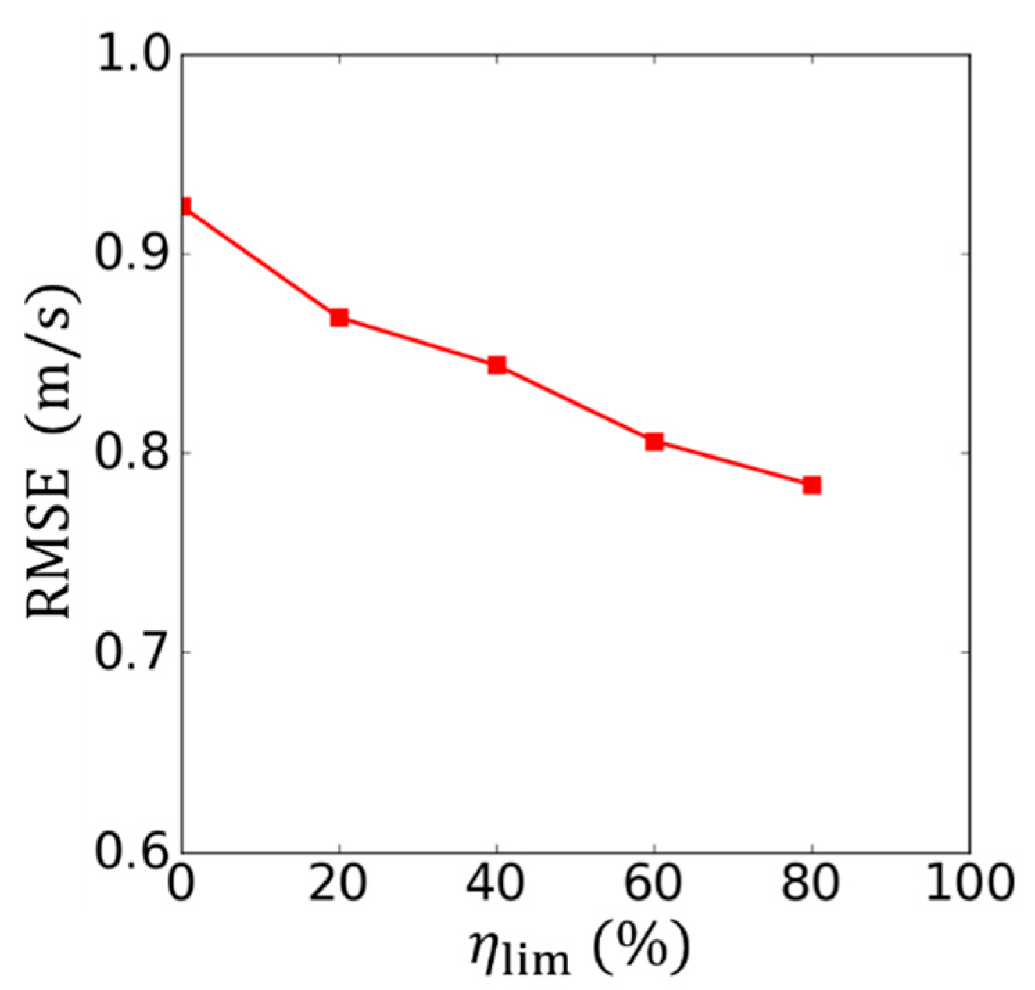
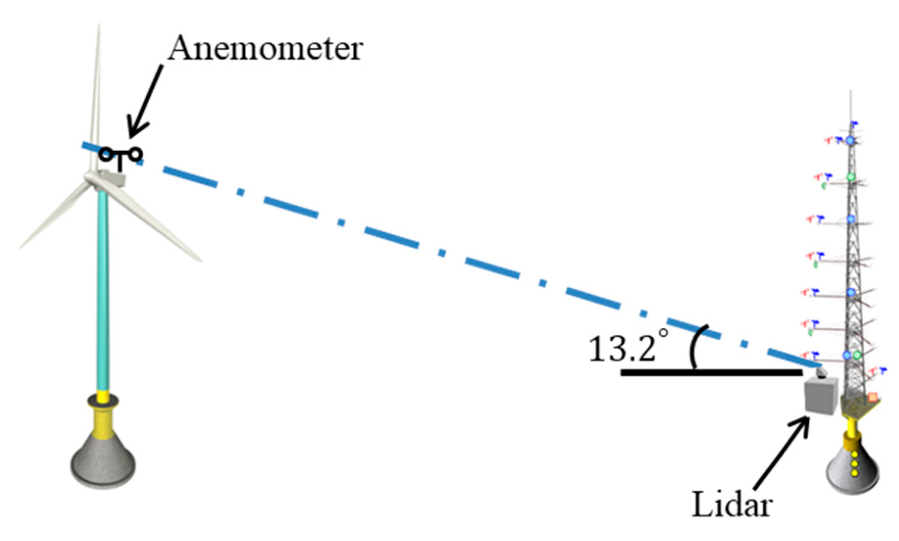
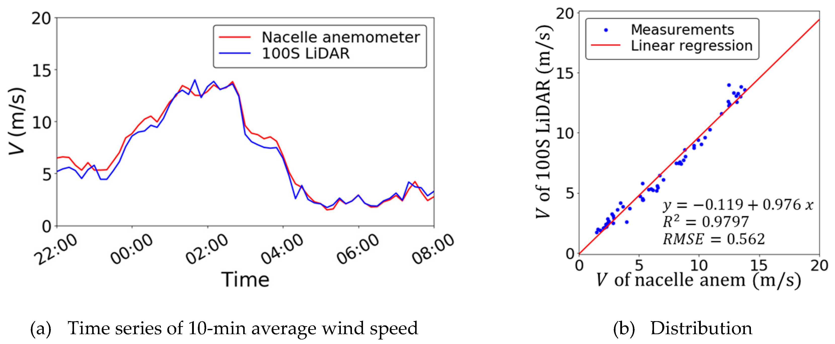
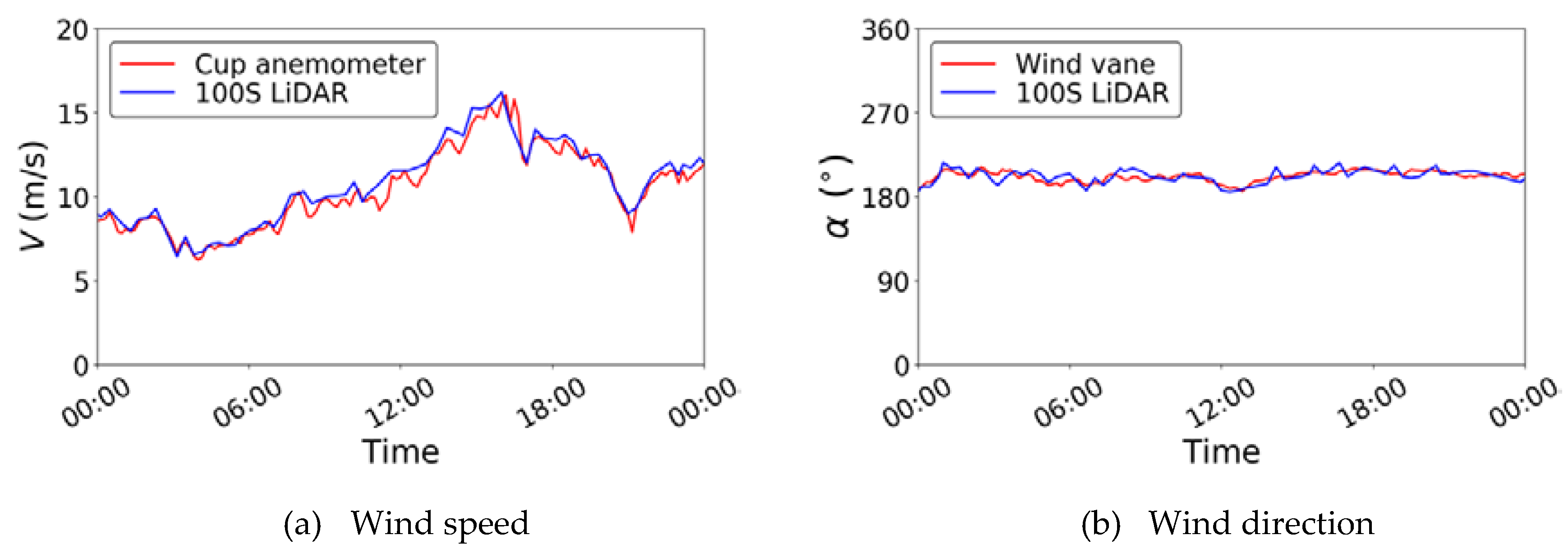
3.2. Validation of Velocity Vector Retrieved from PPI and RHI Scan Data

This section presents validation of the two approaches –proposed in Section 2.2—for retrieving velocity vector from LOS velocity fields obtained in the PPI and RHI scans. The first approach, which requires wind direction information (cf. Equations (4) and (5)), is validated against measurements from the anemometer mounted on the nacelle of the neighboring wind turbine (see Figure 1). A PPI scan is employed to collect scanning LiDAR measurements, as shown in Figure 12. The LiDAR beam is swept at $\varnothing ={13.2}^{°}$ and for an azimuth angle range of 40°, such that the beam passes through the nacelle anemometer, and the wind turbine is in the middle of the azimuth range. In order to obviate the effect of the turbine wake on the nacelle measurement, the comparison was made when the turbine was stopped.

Since the nacelle anemometer-measured wind speed is influenced by the rotor or the shape of the nacelle, the measurement of the nacelle anemometer is first compared against the wind speed measured by cup anemometers installed at a height of 80 m on the meteorological tower. The comparison showed that on average, the wind speed measured by the nacelle anemometer is 5.7% higher than that obtained from the meteorological tower measurement [19]. Therefore, the measurement of the nacelle anemometer is corrected using the velocity ratio 1.057.

Figure 13 shows a comparison of 10-min-averaged wind speeds retrieved from the scanning LiDAR measurement against the measurements of the nacelle-mounted anemometer. The time series and scatter plots show a good agreement between the two measurements with $R^2=0.979$, $\mathrm{RMSE}=0.562$, and slope being 0.976.

Figure 14 and Figure 15 show comparisons of the wind speed and wind direction obtained by scanning Doppler LiDAR (retrieved using the VAD technique) against the wind speed and wind direction measured by the met mast tower. The comparison height is 90 m. Both the time series and scatter plot show a good agreement between the two measurements. The coefficient of determination is $R^2=0.99$ for both wind speed and wind direction, and the RMSE of wind speed is 0.31 m/s, whereas that of wind direction is 5.6°. However, it should be mentioned that the complete conical scan required by this approach can significantly reduce the data sample. Furthermore, due to uncertainty in the LiDAR measurement, it may be necessary to perform multiple scans for the same elevation angle in order to obtain accurate wind directions. This makes the approach less attractive for constructing the velocity field. The current study employs the former approach validated in this section for velocity field reconstruction.

3.3. Measurement and Prediction of Wind Field in Near-Shore Boundary Layer

In order to evaluate the effect of coastal terrain on the near-shore marine ABL, the wind field between the meteorological tower and the coastline was measured. RHI scans were conducted towards the north and for an elevation angle range of 0° to 60°. The wind direction information required by Equation (5) to construct wind speeds from LiDAR-measured LOS velocities ($u_r$) was obtained from a wind vane mounted on the meteorological tower. Furthermore, for the spatial averaging, the measurement data was divided into vertical grids along the north south direction. The size of each block in the grid was set to $50\times 50{\mathrm{m}}^2$. Average wind speeds were computed from all the measurement points in that block and for a fairly long time span of three hours.

Figure 16 shows the mean velocity field in the vertical plane between the observation tower and the northern coast. The left side of the color map is 1000 m from the coast, and the LiDAR is 3500 m from the coast. Strong shear can be observed in the region close to the coast. The coastline has a vertical cliff of about 50 m above the sea level. This enforces the development of an internal boundary layer (IBL) that persists approximately up to 1500 m from the LiDAR position (almost 2 km from the shore).

Figure 17 presents average boundary layer profiles at distances 900 m, 1900 m, and 2900 m from the coastline. All data between 18 November 2016 and 25 December 2016 for which the wind directions were within the limit of $\pm {10}^{°}$ from the north were averaged to produce these profiles. It can be appreciated that the simulations are able to produce more or less similar velocity magnitudes as the measurements. However, for the profiles at 900 m from the coast, i.e., closest to the coast, the difference between the measurement and simulations is significant. Difference between the simulations and the measurements is around 10% up to 500 m. Note that the height where the error line is broken in Figure 17a corresponds to the location where no measurement data was available. For Figure 17b,c, which are further from the coastline, LiDAR measurements are well reproduced by the profiles predicted by the WRF simulations up to a height of 250 m. However, as was the case for the wind blowing from the land (cf. Figure 9c), for higher altitudes, the simulations overestimate the measurement, for the current measurement period.

Until now, results from mesoscale simulations were mainly validated against tower-mounted anemometers or profiling LiDAR with a lower range. Therefore, it was only possible to confirm the accuracy of the simulation results at 200 m or below. By using scanning Doppler LiDAR, together with the proposed method for the reconstruction of the velocity field from LOS velocities, it is now possible to validate the mesoscale simulations against measurements for higher altitudes and different locations in the IBL.

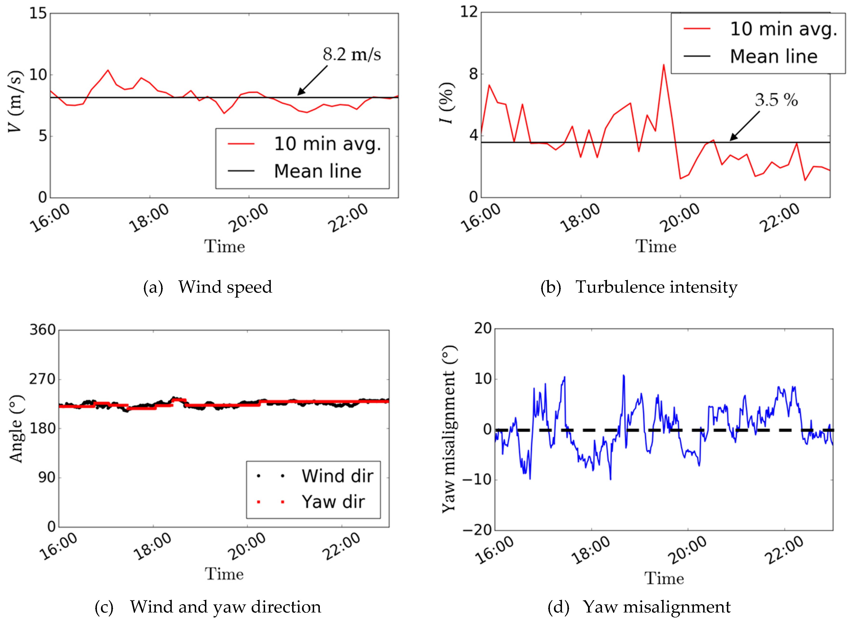
3.4. Measurement and Prediction of Wind Turbine Wake

In this section, the flow field around the wind turbine is measured in order to characterize the wind turbine wake. Measuring the wind turbine wake using scanning Doppler LiDAR poses several challenges. In addition to a low sampling rate, PPI scans conducted using LiDAR can only provide measurements in conical planes. An alternative can be to conduct multiple RHI scans, but this method can only be applied when LiDAR is located in the wake of the turbine, and the wind direction does not vary too much. In this study, multiple PPI scans are performed for a sequence of elevation angles. Figure 18 shows a schematic of this scan approach. From the measured LOS velocities, only those at the hub height level are extracted (the grey plane in Figure 18). Wind speed is then constructed from the LOS velocity using Equation (5).

Figure 19 visualizes the mean flow field around the wind turbine reconstructed from the PPI scans. A velocity deficit, which is a common characteristic of a turbine wake, is clearly visible in the figure. Furthermore, a dual peak is also observed in the near-wake region up to $x/D=2$. It can be appreciated that the wake region persists approximately 7D downstream from the wind turbine. Note that, for $x/D\approx 2$, the azimuth angles are approximately perpendicular to the incoming flow and, therefore, the measurement error is high in this region.

Several other studies have performed scanning Doppler LiDAR-based measurements of wind turbine wakes. However, reconstruction of velocity fields from LiDAR-measured LOS velocities poses a great challenge. Therefore, most of the studies simply tried to analyze and interpret LOS velocities, and did not perform any further processing of the measured data [26,27,28]. As is also mentioned in the Introduction, the assumption of constant wind direction assumption during the measurement period and the application of multiple LiDARs are also receiving a lot of interest in the wind energy community [29,30]. The method of wind turbine wake measurement with a single Scanning Doppler LiDAR for arbitrary directions proposed in this study is therefore different from those in the literature.

Finally, the measurement data is compared against four analytical wake models proposed by Jensen [31], Frandsen et al. [32], Bastankhah and Porte-Agel [33], and Qian and Ishihara [34]. As with most other wake models, the wake models validated in this study require one or more of the following three input parameters: mean inflow velocity, inflow turbulence intensity, and thrust coefficient ($C_T$) of the turbine. The inflow wind speed and turbulence intensity measured by the met mast at the hub height levels are used. Figure 20a,b show the time series of the 10-min-averaged wind speed and turbulence intensity. The average inflow velocity during the comparison period was 8.2 m/s, and the turbulence intensity was 3.5%. From the $C_T-u$ characteristic of the turbine, a thrust coefficient value of 0.8 was used [35]. Figure 20c shows one-minute-averaged wind directions and yaw directions of the turbine during the period when the wind turbine wake data was collected. Figure 20d shows the yaw misalignment. The distribution of the yaw misalignment during the evaluation period was roughly symmetrical on the two sides of 0° and the maximum yaw error was ±10°. The wake model proposed by Qian and Ishihara [34] is able to account for the yaw misalignments. Therefore, for an accurate comparison, the yaw error distribution is used to construct weighted average velocity profiles from this wake model.

Note that Jensen’s model, which assumes top-hat distribution of velocity deficit, is simply a function of $C_T$ and downstream distance from the turbine. The model proposed by Frandsen et al. [32] is based on the conservation of mass and momentum but is also a function of $C_T$ and assumes top-hat velocity deficit distribution. In the model by Bastankhah and Porte-Agel [33], they employed Gaussian distribution to represent velocity deficit profiles. Although the model of Qian and Ishihara also employed Gaussian distribution for velocity deficit, the model and the wake growth rates are the function of both $C_T$ and inflow turbulence intensity.

Figure 21 shows the horizontal profiles of normalized velocity deficit at the hub height in the wake of the wind turbine. Here, the normalized velocity deficit is defined as:

$$\frac{\Delta \mathrm{U}}{U_{0,\mathrm{h}}}=\frac{U_{0,h}-U}{U_{0,h}},$$

(7)

where $U_{0,\mathrm{h}}$ is the average inflow velocity which is equal to 8.2 m/s during the current comparison period, $U$ is the streamwise velocity, and $\mathsf{\Delta }\mathrm{U}$ is the velocity deficit. Profiles obtained from scanning LiDAR are compared with those predicted by the wake models. The models of Jensen and Frandsen et al. underestimate the velocity deficit—compared to the measurement—around the wake center. Similar tendency has been observed in other studies on comparison of these two wake models with the large-eddy simulations (LES) (see, e.g., Ref. [33]). The performance of these models can be further improved by tuning the wake growth rate parameter, as done in some other studies (see Ref. [36] for the review), but the top-hat assumption of velocity deficit will never allow them to reproduce the Gaussian nature of the measured profiles. It can be appreciated that the velocity-deficit profiles predicted by the models of Bastankhah and Porte-Agel and Qian and Ishihara show similar trend as the measured profiles. The model of Bastankhah and Porte-Agel, however, overestimates the velocity deficit at x/D =1 and significantly underestimates the profiles further downstream. The discrepancy can be attributed to the fact that, in this study, the wake growth rate parameters were not obtained from fitting them to the current measurements, instead the parameters from the closest LES case in Ref. [33] were used. The model of Qian and Ishihara shows the most favorable agreement with the measured profiles, though even this model visibly overestimate or underestimate the velocity deficit compared to the measured profiles. The velocity deficit is maximum at $x/D=3$, though a deficit can be observed even at $x/D=6$. At $x/D=1.0$, close to the rotor, a horizontal profile with a dual peak can be observed in the measurement. This dual peak is the result of an uneven distribution of force on the rotor in the radial direction. The near-wake flow is significantly affected by the specific blade aerodynamics, especially when the ambient turbulence is low. This has also been observed in experimental studies as shown by Ishihara and Qian [37]. However, these differences between the wake model and measurements in the near wake region are not very relevant when considering engineering applications of the model. The reason being that the turbine spacing in actual wind farms is always larger than $3\mathrm{D}$, and, in most cases, the streamwise spacing is larger than $7\mathrm{D}$ [38].

4. Conclusions

The current work evaluated the performance of scanning Doppler LiDAR for wind resource measurement and analysis for wind energy applications. The measurement results were also compared with WRF simulations and wake models.

Firstly, 10-min-averaged wind speeds measured by scanning LiDAR in DBS mode were validated against the measurements of an existing V1 LiDAR. It was observed that the quality of measurements degraded when the minimum threshold value of the CNR was increased. As a result, the agreement between the scanning LiDAR and the V1 LiDAR measurements was better when the availability of the scanning LiDAR was higher. However, even with a lower availability of 20% (30 data per 10 min), fairly good 10-min-averaged wind speed data could be produced. Vertical wind profiles were measured in DBS-mode and then investigated for wind blowing from the land and that from the sea. It was found that the wind speed was higher when the wind was blowing from the sea than when it was blowing from the land. The simulated wind profiles by WRF showed a similar tendency to the LiDAR measurements, but they overestimated the measurements at higher altitudes when the wind was blowing from the land.

A method for the reconstruction of wind speeds from conical and slice scans (also known as PPI and RHI) was proposed in this study. The method assumes the wind direction at every point in a scan to be the same as that measured by another wind vane. The proposed velocity retrieval method with RHI and wind directions obtained from the wind vane mounted on the meteorological tower was then used to investigate the effect of coastal terrain on the ABL by measuring the flow field between the LiDAR and the coastline. The coastal terrain was responsible for the development of an IBL resulting in strong shear in the region close to the coast. It was also found that this IBL persisted for approximately 2000 m offshore.

Finally, the flow field around the wind turbine was measured using multiple PPI scans together with wind directions obtained from the wind vane mounted on the meteorological tower and processed to characterize the wind turbine wake. A velocity deficit in the wind turbine wake was clearly visible along with a dual peak in the near-wake region in the flow field visualization. Horizontal profiles of velocity deficit in the wake of the wind turbine showed common characteristics observed in earlier numerical and experimental studies. The LiDAR measurement was also used to validate the wake models. Two of the Gaussian wake models showed better agreement with the measurements than the models with top-hat velocity distribution.

References

1. Holleman, I. Quality control and verification of weather radar wind profiles. J. Atmos. Ocean. Technol. 2005, 22, 1541–1550. [Google Scholar] [CrossRef] [Green Version]
2. Browning, K.A.; Wexler, R. The determination of kinematic properties of a wind field using Doppler radar. J. Appl. Meteorol. Climatol. 1968, 7, 105–113. [Google Scholar] [CrossRef]
3. Holleman, I. Doppler Radar Wind Profiles; Roya Netherlands Meteorological Institute (KNMI): De Bilt, The Netherlands, 2003. [Google Scholar]
4. Smith, D.A.; Harris, M.; Coffey, A.S.; Mikkelsen, T.; Jørgensen, H.E.; Mann, J.; Danielian, R. Wind lidar evaluation at the danish wind test site in Høvsøre. Wind Energy 2006, 9, 87–93. [Google Scholar] [CrossRef]
5. Lang, S.; McKeogh, E. LIDAR and SODAR measurements of wind speed and direction in upland terrain for wind energy purposes. Remote Sens. 2011, 3, 1871–1901. [Google Scholar] [CrossRef] [Green Version]
6. Goit, J.P.; Shimada, S.; Kogaki, T. Can LiDARs replace meteorological masts in wind energy? Energies 2019, 12, 3680. [Google Scholar] [CrossRef] [Green Version]
7. Kelley, N.D.; Jonkman, B.J.; Scott, G.N. Comparing Pulse Doppler LIDAR with SODAR and Direct Measurements for Wind Assessment. In Proceedings of the American Wind Energy Association WindPower 2007 Conference and Exhibition, Los-Angeles, CA, USA, 3–7 June 2007; p. 20. [Google Scholar]
8. Pichugina, Y.L.; Banta, R.M.; Brewer, W.A.; Sandberg, S.P.; Hardesty, R.M. Doppler Lidar-based wind-profile measurement system for offshore wind-energy and other marine boundary layer applications. J. Appl. Meteorol. Climatol. 2012, 51, 327–349. [Google Scholar] [CrossRef]
9. Gottschall, J.; Courtney, M. Verification Test for Three WindCube WLS7 LiDARs at the Høvsøre Test Site; Tech. Rep. Risø-R-1732; Technical University of Denmark: Roskilde, Denmark, 2010. [Google Scholar]
10. Easterbrook, C.C. Estimating horizontal wind fields by two-dimensional curve fitting of single doppler radar measurements. In Proceedings of the Radar Meteorology Conference, Huston, TX, USA, 22–24 April 1975. [Google Scholar]
11. Waldteufel, P.; Corbin, H. On the analysis of single-doppler radar data. J. Appl. Meteorol. 1978, 18, 532–542. [Google Scholar] [CrossRef]
12. Koscielny, A.J.; Doviak, R.J.; Rabin, R. Statistical considerations in the estimation of divergence from single-Doppler radar and application to prestorm boundary-layer observations. J. Appl. Meteorol. 1982, 21, 197–210. [Google Scholar] [CrossRef] [Green Version]
13. Banta, R.M.; Newsom, R.K.; Lundquist, J.K.; Pichugina, Y.L.; Coulter, R.L.; Mahrt, L. Nocturnal low-level jet characteristics over Kansas during cases-99. Bound. Layer Meteorol. 2002, 105, 221–252. [Google Scholar] [CrossRef]
14. Iungo, G.V.; Porte-Agel, F. Volumetric lidar scanning of wind turbine wakes under convective and neutral atmospheric stability regimes. J. Atmos. Ocean. Technol. 2014, 31, 2035–2048. [Google Scholar] [CrossRef]
15. Mann, J.; Cariou, J.P.; Courtney, M.S.; Parmentier, R.; Mikkelsen, T.; Wagner, R.; Lindelöw, P.; Sjöholm, M.; Enevoldsen, K. Comparison of 3D turbulence measurements using three staring wind lidars and a sonic anemometer. Meteorol. Z. 2009, 18, 135–140. [Google Scholar] [CrossRef]
16. Fuertes, F.C.; Iungo, G.V.; Porte-Agel, F. 3D turbulence measurements using three synchronous wind lidars: Validation against sonic anemometry. J. Atmos. Ocean. Technol. 2014, 31, 1549–1556. [Google Scholar] [CrossRef]
17. Windcube Windcube 100s/200s/400s—3D Wind Doppler LIDAR. Available online: http://www.leosphere.com/wp-content/uploads/2016/12/WINDCUBE-Scannant-Brochure-4p-20151116-HD.pdf (accessed on 23 August 2019).
18. Kikuchi, Y.; Fukushima, M.; Ishihara, T. Assessment of a coastal offshore wind climate by means of mesoscale model simulations considering high-resolution land use and sea surface temperature data sets. Atmosphere 2020, 11, 379. [Google Scholar] [CrossRef] [Green Version]
19. Goit, J.P.; Yamaguchi, A.; Ishihara, T. Performance Evaluation of Scanning Doppler Lidar and its Application to Wind Field Measurement. Tech. Rep. Japan Wind Energy Assoc. 2018, 42, 7–16. (In Japanese) [Google Scholar]
20. Clifton, A. Remote Sensing of Complex Flows by Doppler Wind Lidar: Issues and Preliminary Recommendations; Tech. Rep. NREL/TP-5000-64634; National Renewable Energy Laboratory: Golden, CO, USA, December 2015.
21. Skamarock, W.C.; Klemp, J.B.; Dudhia, J.; Gill, D.O.; Barker, D.M.; Duda, M.G.; Huang, X.-Y.; Wang, W.; Powers, J.G. A description of the advanced research WRF version 3. Tech. Rep. NCAR 2008, NCAR/TN–47, 1–113. [Google Scholar]
22. Iizuka, S. Future environmental assessment and urban planning by downscaling simulations. J. Wind Eng. Ind. Aerodyn. 2018, 181, 69–78. [Google Scholar] [CrossRef]
23. Yoshie, R.; Miura, S.; Mochizuki, M. Validation of WRF for preparation of standard wind data validation of WRF for preparation of standard wind data for assessment of pedestrian wind environment. J. Wind Eng. JAWE 2015, 40, 113–122, [In Japanese]. [Google Scholar] [CrossRef]
24. NOAA Earth System Research Laboratory. NCEP Reanalysis Data Provided by the NOAA/OAR/ESRL PSD, Boulder, Colorado, USA. 2017.5. Available online: https://www.esrl.noaa.gov/psd/ (accessed on 10 August 2019).
25. Stark, J.D.; Donlon, C.J.; Martin, M.J.; McCulloch, M.E. OSTIA: An operational, high resolution, real time, global sea surface temperature analysis system. In Proceedings of the OCEANS 2007—Europe, Aberdeen, UK, 18–21 June 2007; pp. 1–4. [Google Scholar]
26. Aitken, M.L.; Banta, R.M.; Pichugina, Y.L.; Lundquist, J.K. Quantifying wind turbine wake characteristics from scanning remote sensor data. J. Atmos. Ocean. Technol. 2014, 31, 765–787. [Google Scholar] [CrossRef]
27. Smalikho, I.N.; Banakh, V.A.; Pichugina, Y.L.; Brewer, W.A.; Banta, R.M.; Lundquist, J.K.; Kelley, N.D. Lidar investigation of atmosphere effect on a wind turbine wake. J. Atmos. Ocean. Technol. 2013, 30, 2554–2570. [Google Scholar] [CrossRef]
28. Banta, R.M.; Pichugina, Y.L.; Brewer, W.A.; Lundquist, J.K.; Kelley, N.D.; Sandberg, S.P.; Alvarez, R.J.; Hardesty, R.M.; Weickmann, A.M. 3D volumetric analysis of wind turbine wake properties in the atmosphere using high-resolution Doppler lidar. J. Atmos. Ocean. Technol. 2015, 32, 904–914. [Google Scholar] [CrossRef]
29. Iungo, G.V.; Porté-Agel, F. Measurement procedures for characterization of wind turbine wakes with scanning Doppler wind LiDARs. Adv. Sci. Res. 2013, 10, 71. [Google Scholar] [CrossRef] [Green Version]
30. Newsom, R.K.; Berg, L.K.; Shaw, W.J.; Fischer, M.L. Turbine-scale wind field measurements using dual-Doppler lidar. Wind Energy 2015, 18, 219–235. [Google Scholar] [CrossRef]
31. Jensen, N.O. A Note on Wind Generator Interaction; Tech. Rep. Riso-M-2411; Riso National Laboratory: Roskilde, Denmark, November 1983. [Google Scholar]
32. Frandsen, S.; Barthelmie, R.J.; Pryor, S.; Rathmann, O.; Larsen, S.; Højstrup, J.; Thøgersen, M. Analytical modelling of wind speed deficit in large offshore wind farms. Wind Energy 2006, 9, 39–53. [Google Scholar] [CrossRef]
33. Bastankhah, M.; Porté-Agel, F. A new analytical model for wind-turbine wakes. Renew. Energy 2014, 70, 116–123. [Google Scholar] [CrossRef]
34. Qian, G.-W.; Ishihara, T. A new analytical wake model for yawed wind turbines. Energies 2018, 11, 665. [Google Scholar] [CrossRef] [Green Version]
35. Yamaguchi, A.; Widyasih, S.P.; Ishihara, T. Load Estimation of a Wind Turbine Support Structure during Operation and Validation by Measurement. In Proceedings of the 23rd Wind Engineering Symposium, Tokyo, Japan, 3–5 December 2014; pp. 133–138. [Google Scholar]
36. Porté-Agel, F.; Bastankhah, M.; Shamsoddin, S. Wind-turbine and wind-farm flows: A Review. Bound. Layer Meteorol. 2019, 174, 1–59. [Google Scholar] [CrossRef] [Green Version]
37. Ishihara, T.; Qian, G. A new Gaussian—Based analytical wake model for wind turbines considering ambient turbulence intensities and thrust coefficient effects. J. Wind Eng. Ind. Aerodyn. 2018, 177, 275–292. [Google Scholar] [CrossRef]
38. Stevens, R.J.A.M.; Gayme, D.F.; Meneveau, C. Effects of turbine spacing on the power output of extended wind-farms. Wind Energy 2016, 19, 359–370. [Google Scholar] [CrossRef] [Green Version]
Figure 1. Choshi offshore wind energy test facility. (a) Google map, (b) picture of wind turbine and the met mast tower.
Atmosphere 11 00442 g001
Figure 2. Schematic representation of the Doppler beam swinging (DBS) configuration.
Atmosphere 11 00442 g002
Figure 3. Schematic of two scan modes (a,b) used for wind field measurements.
Atmosphere 11 00442 g003
Figure 4. u r as a function of azimuth angle ( θ ) for elevation angle ( ϕ ) = 50°and range of 100 m. Red circles indicate peak u r .
Atmosphere 11 00442 g004
Figure 5. Distribution of Carrier-to-Noise-Ratio (CNR) for the measurements at the height of 140 m. Period: 1 April 2016 to 15 April 2016.
Atmosphere 11 00442 g005
Figure 6. Comparison of 10-min-average wind speeds of scanning Doppler LiDAR and V1 LiDAR at 140 m height for different CNR thresholds (ac).
Atmosphere 11 00442 g006
Figure 7. Root mean square error between scanning Doppler LiDAR and V1 LiDAR at 140 m plotted as a function of η lim .
Atmosphere 11 00442 g007
Figure 8. (a) Number of data measured every 10 min at different heights for the period of two weeks from 1 April 2016 to 15 April 2016. Horizontal lines indicates η lim = 80 % . (b) Data availability profiles for various η lim values. Horizontal line indicates the hub height of the wind turbine installed at the site.
Atmosphere 11 00442 g008
Figure 9. Vertical profiles of horizontal velocity for wind blowing from the land and that from the sea (for May 2016). Horizontal dashed lines indicate the hub height level, and the dark profiles indicate the percentage error in the Weather Research and Forecasting (WRF) profiles compared to the LiDAR measurement.
Atmosphere 11 00442 g009
Figure 10. Comparison of the diurnal cycle of vertical profiles of horizontal velocity for wind blowing from the land and that from the sea (for May 2016).
Atmosphere 11 00442 g010
Figure 11. (a,b) Comparison of hourly averaged profiles of horizontal velocity which are further averaged over the period of one-month (for May 2016). Horizontal dashed lines indicate the hub height level, and the dark profiles indicate the percentage error in the WRF profiles compared to the LiDAR measurement.
Atmosphere 11 00442 g011
Figure 12. Schematic of the LiDAR beam targeting the nacelle-mounted anemometer. The scan is performed in the plan-position indicator (PPI) mode for validating the proposed velocity retrieval approach.
Atmosphere 11 00442 g012
Figure 13. Validation of the scanning LiDAR-measured mean wind speeds against those obtained from the nacelle-mounted anemometer (a). Measurement data (b) collected from 25 October 2016 22:00 to 26 October 2016 8:00.
Atmosphere 11 00442 g013
Figure 14. Comparison of the time series of wind speed (a) and wind direction (b) of scanning Doppler LiDAR (retrieved using velocity azimuth display (VAD)) and met mast tower at 90 m height (on 6 September 2016).
Atmosphere 11 00442 g014
Figure 15. Comparison of 10-min-averaged wind speed and wind direction of scanning Doppler LiDAR (retrieved using VAD) and met mast tower at 90 m height (September 2016).
Atmosphere 11 00442 g015
Figure 16. Visualization of wind fields measured in the vertical plane from LiDAR position towards the coast. Vertical dashed lines indicate positions where velocity profiles are plotted in Figure 17. Measurement data collected on 28 November 2016 from 12:00 to 15:00.
Atmosphere 11 00442 g016
Figure 17. Comparison of vertical profiles of WRF simulations against the LiDAR measurements at three different locations from the coast (ac). Horizontal dashed lines indicate the hub height level, and the dark profiles indicate the percentage error in the WRF profiles compared to the LiDAR measurement. Data is from 18 November 2016 to 25 December 2016.
Atmosphere 11 00442 g017
Figure 18. Schematic of the multiple PPI scans for the measurement and reconstruction of flow field around wind turbine. Wind speed data is extracted in the grey horizontal plane at the hub height level.
Atmosphere 11 00442 g018
Figure 19. Visualization of horizontal mean wind field at hub height obtained from PPI scans collected on 28 September 2016 from 16:00 to 22:45. Vertical dashed lines indicate axial positions where profiles are plotted in Figure 21.
Atmosphere 11 00442 g019
Figure 20. (a,b): Time series of 10-min-averaged wind speed and turbulence intensity at the height of 90 m measured by the met mast. The dark lines are mean wind speed and turbulence intensity over the time range. (c) Time series of one-minute-averaged wind and yaw directions at the wind turbine nacelle. (d) Time series of yaw misalignment.
Atmosphere 11 00442 g020
Figure 21. Horizontal profiles of normalized velocity deficit at the hub height level and at various downstream locations of the wind turbine wake. Top figure shows horizontal profile of mean wind speed 1 D upstream from the turbine. LiDAR measurement data from 28 September 2016 from 16:00 to 22:45.
Atmosphere 11 00442 g021