Article

Comparison of Remote Sensing based Multi-Source ET Models over Cropland in a Semi-Humid Region of China

1
College of Geomatics Science and Technology, Nanjing Tech University, Nanjing 211816, China
2
Chinese Academy of Surveying and Mapping, No.28 Lianhuachi West Road, Haidian District, Beijing 100036, China
*
Author to whom correspondence should be addressed.
Atmosphere 2020, 11(4), 325; https://doi.org/10.3390/atmos11040325
Submission received: 28 February 2020 / Revised: 23 March 2020 / Accepted: 24 March 2020 / Published: 27 March 2020
(This article belongs to the Section Biosphere/Hydrosphere/Land–Atmosphere Interactions)

Abstract

:
The estimation of cropland evapotranspiration (ET) is essential for agriculture water management, drought monitoring, and yield forecast. Remote sensing-based multi-source ET models have been widely applied and validated in the semi-arid region of China. However, careful investigation of the models’ performances for different crop types (winter wheat and summer maize) over the semi-humid region is still necessary. This study used remote sensing data (Landsat 8 and ASTER) and compared three mainstream multi-source ET models: (i) the two-source energy balance model, i.e., TSEB; (ii) the Penman-Monteith based four-source model, i.e., 4s-PM; (iii) the Priestley Taylor-Jet Propulsion Laboratory ET algorithm, i.e., PT-JPL. The measurements of the eddy-covariance (EC) flux tower located in Guantao county of North China were used to validate the models. The results showed that the TSEB model performed the best in estimating latent heat flux (LE) of maize, with an RMSE of 75.0 W/m2 and an R2 of 0.9, and the 4s-PM model had the highest accuracy of LE estimation for wheat, with an RMSE of 61.0 W/m2 and an R2 of 0.91. The LE spatial distribution comparison indicated that the PT-JPL model had more capacity to exhibit crop ET heterogeneity. The major environmental factors affecting ET varied with crop types and crop growth stages. Without taking soil moisture into account, the 4s-PM and TSEB models overestimated LE under water deficit in the maturation stage of wheat. The plant moisture stress based on vegetation index in the PT-JPL model underestimated the evaporation in the maturation stage while the cropland was still wet.

1. Introduction

Land surface evapotranspiration (ET) combines vegetation transpiration and soil evaporation, it is a crucial component of the interaction between the surface and atmosphere and is the major part of the global water cycle [1]. In agriculture, reliably determining ET is the premise for calculating the water use efficiency of crops and optimizing agriculture water management [2]. At a local scale, ET can be measured by pan evaporation, lysimeter, Bowen ratio, eddy covariance (EC) and large aperture scintillometer (LAS). An EC system can provide continuously precise measurements of water vapor flux over a homogeneous surface and is very popular for parameter optimization and validation in numerous researches of land surface models [3,4,5,6,7,8]. However, the ground-based measurements are limited for their spatial representation and the high cost; when the research scale is larger, these methods do not apply [9]. Remote sensing technology plays a vital role in ET estimation because it can provide many parameters needed in ET models at regional scales, such as land surface temperature, surface albedo, and vegetation indexes. Nowadays, mainly when higher-resolution optical and thermal infrared sensors have emerged, the broad utility of remote sensing techniques in ET estimation has shown excellent application prospects.
The remote sensing-based single-source energy balance models such as the Surface Energy Balance Algorithm for Land (SEBAL) [5] and Surface Energy Balance System (SEBS) [6], treat the surface as a big leaf and use land surface radiometric temperature from satellites to derive sensible heat flux. However, theoretically, the air temperature at the source/sink level, which is called aerodynamic temperature and can be significantly different from radiometric temperature, is responsible for the transfer of heat from the surface to the atmosphere [10,11,12,13]. For partial canopy cover surface, the soil temperature has a significant impact on the radiometric surface temperature, whereas the aerodynamic temperature remains closer to a mix of air and vegetation temperatures and is less influenced by the soil temperature [12]. The remote sensing radiometric temperature is always observed at midday; at this time, the soil temperature is generally higher than the vegetation temperature, leading the observed radiometric surface temperature larger than the aerodynamic temperature [12]. In such cases, an ’extra conductance,’ which is estimated based on the dimensionless parameter kB−1, is introduced to compensate for errors arising due to the inequalities between radiometric and aerodynamic temperatures [13,14]. For single-source SEB models, the main limitation lies in the uncertainties of the k−1. The SEBS may underestimate sensible heat flux and overestimate latent heat flux in semi-arid and arid areas for its kB−1 estimation lacks consideration of water stress [15]. The SEBAL is sensitive to the value of kB−1; a fixed value of 2.3 may cause significant errors in sensible heat flux estimation [11].
As many researchers reported, multi-source surface energy balance models are more suitable under partial vegetation canopy cover, because both soil and vegetation components contribute to the net flux exchange as well as the remotely sensed signals [16,17]. The widely used remote sensing-based multi-source ET models contain (i) dual-source energy balance models, such as the Two-Source Energy Balance (TSEB) [3,18] and Atmosphere-Land Exchange Inverse (ALEXI) [4]; (ii) the PM-based models, such as the MOD16 algorithm [7,8]; (iii) the Priestley Taylor-Jet Propulsion Laboratory (PT-JPL) ET algorithm [19,20] and so on. The TSEB requires the input of the component temperatures (soil and canopy temperatures), and the Priestley-Taylor iteration approach, which derives the component temperatures by providing an initial estimate of the canopy transpiration, are adopted to solve TSEB. The ALEXI model was developed as a robust regional framework, which coupled the TSEB with an atmospheric boundary layer (ABL) model to internally simulate the land-atmosphere feedback of air temperature used as a boundary condition to a sensible heat component [21]. The PM-based multi-source model, such as the MOD16 algorithm, considers the different ET processes of wet canopy evaporation, canopy transpiration, moist soil, and saturated soil evaporation. The PT-JPL model uses environmental constraint factors estimated using empirical formulas to scale an equilibrium ET to the actual ET.
There are still limitations in multi-source ET algorithms; for the TSEB model, the Priestley-Taylor iteration does not include a reasonable reduction of initial canopy transpiration. As many types of research articles reported, the TSEB may overestimate the latent heat flux and underestimate the sensible heat flux, especially under vegetative stress conditions in arid or semi-arid regions [17]. The accuracy of PM-based ET models depends on the soil and canopy resistances estimation, which are affected by environmental factors such as soil moisture, vapor pressure, air temperature, and solar radiation [22]. The PT-JPL model is easy to use because it does not need the input of aerodynamic or stomatal resistance. However, such a simplification may lead to a significant bias if there is a saturated evaporating front (i.e., after a heavy rainfall event or irrigation) [23]. Furthermore, with the lack of aerodynamic conductance, the PT-JPL model and empirical models do not thoroughly explain the phenomenon that the transpiration rate of plants can increase with an increase in the vapor pressure deficit (VPD) under controlled experimental conditions [23,24].
In China, research has focused on validating the multiple-source ET models in the arid or semi-arid area, such as the Heihe river basin [2,16,17,25,26]. The findings of this research give detailed uncertainty evaluation of the ET models. However, the north plain of China, which has a semi-humid climate, is facing a severe water crisis because crops consume much water, and the irrigation intensity is very high [27,28,29]. In such cases, accurately knowing the ET of the cropland is very meaningful for the effective management of water resources. The latest studies mainly focused on using models to obtain spatio-temporal patterns of ET and lacked the internal comparison between them [30,31] over cropland in this region. This paper aimed to comprehensively evaluate the performances of three mainstream multi-source ET models from site to spatial scales, such as the TSEB, 4s-PM, and PT-JPL models, in a semi-humid area of north China, with winter wheat and summer maize as the main crops. Section 2 gives a detailed introduction to the study area, meteorological, and remote sensing data used in this research. Section 3 presents a description of the three multi-source models. Section 4 shows the validation of latent heat fluxes estimated by the three models for different crops and the comparisons of latent heat flux spatial distribution. Section 5 gives a discussion for how the different performances of the three models are attributed to the different model inputs and environmental factors.

2. Study Area and Data

2.1. Site Description and Measurements

The automatic weather station (AWS) and eddy covariance (EC) system (36°30′ N, 117°19′ E) were installed in Guantao county, which is located in the south of the Hebei Province in the Hai Basin (115°06′–115°40′ E, 36°27′–36°47′ N) with a warm temperate, semi-humid, continental monsoon climate. The average annual temperature and precipitation are 14 °C and 548.7 mm, respectively. January is the coldest month with an average temperature of −2.5 °C, while July is the hottest month with an average temperature of 27 °C. Moreover, most of the precipitation occurs from June to September, while little occurs from October to May. The underlying surface of the site is cropland, and the main cultivated crops are winter wheat and maize. The winter wheat grows from October to June and the summer maize from June to October [9,32]. Figure 1a shows the land cover classified using Landsat 8 image in 2014. The photograph of the AWS and EC tower (Figure 1b) in Guantao during the winter wheat growing season showed that the site is flat and homogeneous.
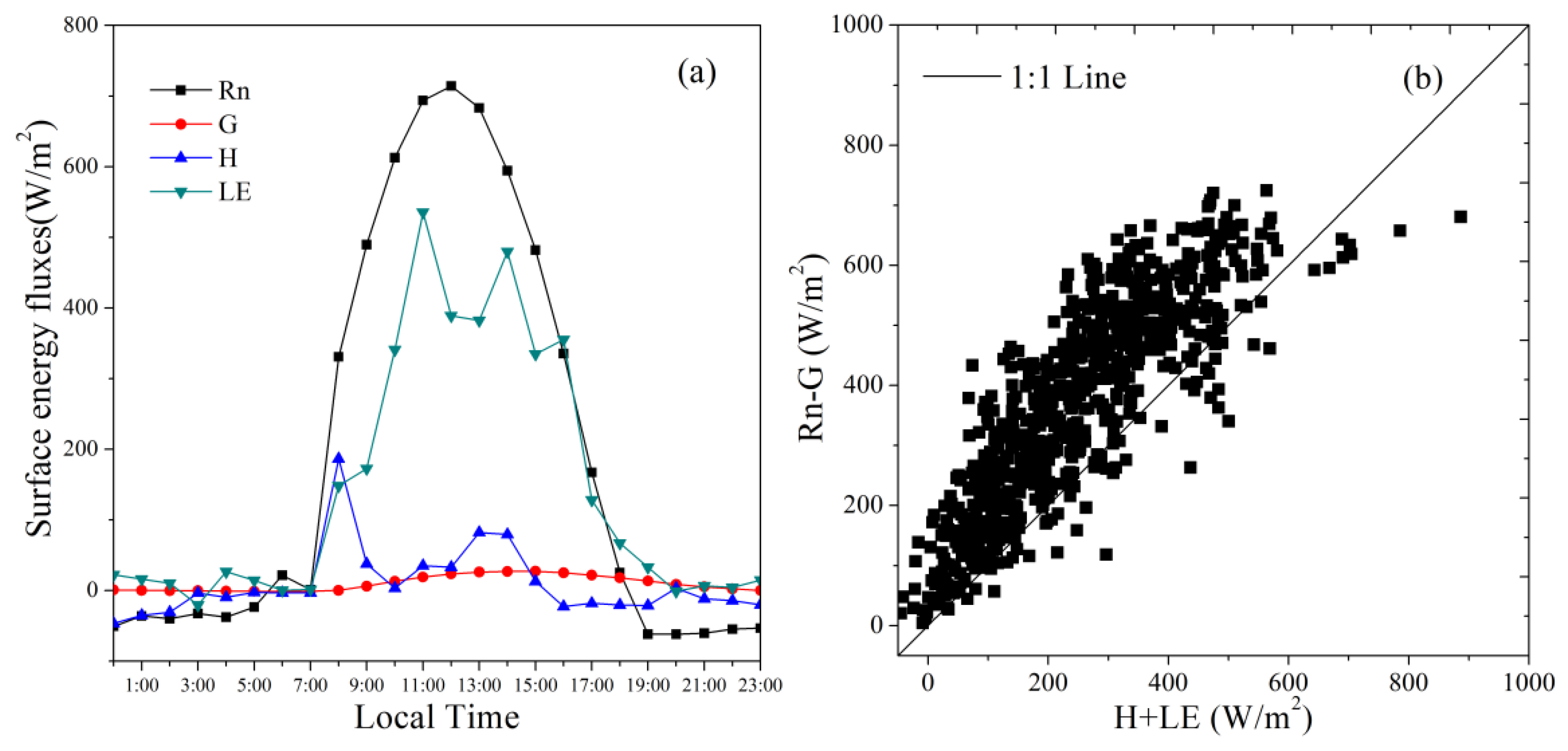
The meteorological and flux data are transferred automatically and simultaneously from the stations to the server. The AWS systems collected data on wind speed, air temperature, and air humidity at the heights of 4 m, 5 m, 8 m, and 15 m every 10-min interval. The surface radiometric temperature, soil heat flux, and four-component of radiation were measured at the same frequency. The EC flux data were averaged every 30 min with the post-processing software EdiRe (University of Edinburgh) and EddyPro (Li-COR Biosciences) [9]. Figure 2 shows the EC measured hourly surface energy fluxes on 18 May 2015 and the surface energy balance closure at the satellite overpass time during 2013–2017. The phenomenon of energy non-closure also existed in this site, which is universal in other research [25,26]. The averaged closure ratio [CR= (LE + H)/(Rn − G)] for all observations was found to be 0.7. Twine et al. [33] reported that the Bowen ratio method for forcing the closure of the measured energy balance improved the agreement with the water balance results. Therefore, this method was used to correct the EC measurements of the sensible and latent heat fluxes for energy closure. Abnormal values were removed because of instrument malfunction and bad weather to guarantee flux data reliability.

2.2. Remote Sensing Data

The Advanced Spaceborne Thermal Emission and Reflection Radiometer (ASTER) was carried on Terra satellite launched on 18 December 1999 and has three spectral bands in the visible near-infrared (VNIR), six bands in the short-wave infrared (SWIR), and five bands in the thermal infrared (TIR) regions. Landsat 8 satellite was launched on 11 February 2013 and carried an operational land imager (OLI) and a thermal infrared sensor (TIRS). Nineteen clear-sky images covering Guantao site from Landsat 8 and two days of land surface temperature (LST) and surface reflectance data from ASTER Level 2 product were collected from https://earthdata.nasa.gov/. Table 1 listed the detail dates and the remote sensing provided data. The overpass time of Landsat 8 and ASTER in Guantao county is around 10:50 a.m. and 11:10 a.m., respectively.
The spectral radiance from Landsat 8 was obtained through a radiometric calibration process and was further atmospheric corrected using the Environment for Visualizing Images (ENVI) Fast Line-of-sight Atmospheric Analysis of Spectral Hypercubes (FLAASH) method to obtain surface reflectance. The ASTER level 2 surface reflectance (AST_07) product provided the surface reflectance in visible and near-infrared. The surface albedo α of Landsat 8 and ASTER was calculated using surface reflectance according to Liang et al. [34]. The Normalized Difference Vegetation Index (NDVI) was computed by the reflectance of near-infrared and red bands.
Surface radiometric temperature (Trad) is the thermal emission from the landscape surface, including vegetated surfaces, as well as other surfaces (such as bare soil). In this study, the Trad for Landsat 8 images was derived from band 10 using the single-channel algorithm developed by Sobrino et al. [35]. The surface emissivity and atmosphere profile data needed in the algorithm was calculated using the NDVI [35] and obtained from the Atmospheric Correction Parameter Calculator of NASA (https://atmcorr.gsfc.nasa.gov/), respectively. The Trad of ASTER was provided by the level 2 surface reflectance (AST_08) product.
All of the images were geometrically rectified to the Universal Transversal Mercator projection (UTM Zone 50N) and resampled to a resolution of 30 m using the cubic convolution method by ENVI.

3. Theory and Methodology

3.1. TSEB Model

The TSEB model was developed initially by Norman et al. [3] and modified by Kustas and Norman [36]. The net radiation Rn, sensible heat flux H, and latent heat flux LE are partitioned between the vegetated canopy and soil and were calculated as:
R n = R n c + R n s = G + H + L E
R n = ( 1 α ) S d + ε a σ T a 4 ε σ T r a d 4
R n c = R n [ 1 exp ( k L A I / 2 cos ( θ z ) ) ]
R n c = L E c + H c
R n s = L E s + H s + G
G = c g R n s
where Rnc and Rns are the canopy and soil net radiation (W·m−2) and the soil heat flux G (W·m−2) in Equation (6) is assumed to be a constant ratio (i.e., cg = 0.35) of Rns [17]. H and LE are the sensible and latent heat flux (W·m−2), respectively. ε is the land surface emissivity, and Sd is the downwelling shortwave radiation (W·m−2) estimated by Allen et al. [37], εa is the emissivity of the atmosphere calculated by air temperature Ta (K) and the water vapor pressure. LAI is the leaf area index and can be calculated by the NDVI [17], θz is the solar zenith angle, and the value of k = 0.45 is adopted for dense vegetated cover (i.e., LAI ≥ 2), while for partial canopy cover, LAI < 2, k = 0.8 is used [18]. The sensible heat fluxes from canopy and soil are estimated by Equations (7) and (8), where ρ is the air density (kg·m−3), Cp is the specific heat of air (J·kg−1·K−1), Tc is the radiometric temperature from the canopy component, and Ts is the radiometric temperature from the soil surface. In TSEB, it is assumed that the remote sensing-based surface radiometric temperature Trad can be related to the sum of vegetation and soil temperatures weighted by the fractional vegetation cover (i.e., Equation (9)). ra,c is the aerodynamic resistance to heat transfer between the canopy and the reference height (see Appendix A of Morillas et al. [38]), and ra,s is the aerodynamic resistance to heat flow in the boundary layer immediately above the soil surface (see Appendix C of Norman et al. [5]):
H c = ρ C p T c T a r a , c
H s = ρ C p T s T a r a , c + r a , s
T r a d = [ f c T c 4 + [ 1 f c ] T s 4 ] 1 4
Tc and Ts are critical for solving the component surface fluxes from canopy and soil, and the Priestley-Taylor method, Equations (4) and (7) compute the initial canopy temperature as Equation (10):
T c i = T a + R n c r a , c ρ C p ( 1 α p t f g Δ Δ + γ )
where Tci is the initial estimate of Tc, fg is the green canopy fraction, the value of αpt for the canopy transpiration under non-stressed conditions is assumed to have a value ~1.26. Δ is the slope of the saturation vapor pressure versus temperature curve, and γ is the psychrometric constant of ~0.066 (Kpa·K−1). Once the Tc is derived, the Hc and Hs can be directly solved by Equations (7)–(9), then LEs is computed using Equations (1)–(5); if the value of LEs is less than zero, an unrealistic situation under daytime conditions is assumed because condensation in the soil is very unlikely. In this case, the αpt is declined, and a new estimate of Tc is adopted to calculate the component fluxes. The procedure is conducted iteratively until the LEs is greater than zero.

3.2. 4s-PM Model

The Penman-Monteith (PM) based 4-s model has the same scheme as the algorithm proposed by Mu et al. [8], it is assumed that there exists no interaction among different ET sources, such as plant transpiration, wet canopy evaporation, saturated soil surface, and moist soil surface evaporation, and the total ET is the sum of the four-source water fluxes. In this model, the plant transpiration LEc,t is computed as:
L E c , t = Δ R n c + ρ C p e s e a r a Δ + γ ( 1 + r c r a ) ( 1 f w e t )
where ra is the aerodynamic resistance to heat transfer (s/m) and computed with the support of aerodynamic roughness, wind speed at reference height, and atmospheric stability correction, rc is the canopy resistance (s/m) for evaporation from the leaves and transpiration from the plant canopy and estimated using Equation (12) based on the Jarvis’s model [22,39] with different environment constraints, the relative surface wetness (ƒwet) is used to determine whether the surface is wet or not following Fisher et al. [19], es is the saturated vapor pressure (Kpa), and ea is the actual vapor pressure (Kpa) estimated by relative humidity Rh. gsmax is the maximum stomatal conductance. In this study, gsmax was set to 0.0025 m/s, which has been widely used for cropland in both local and global water heat flux research [40,41].
r c = 1 g s max f ( s ) f ( T a ) R h L A I
Recent research showed that evaporation from precipitation and irrigation water intercepted by the canopy was a significant contributor toward total ET from the dense canopy. For the wet part of the canopy, several studies suggested that the rc is negligible [42,43] and can be set to zero [24,36]; then, the evaporation for the wet canopy surface is computed as Equation (13):
L E c , e = Δ R n c + ρ C p e s e a r a Δ + γ f w e t
The soil is divided into moist and saturated surfaces in the 4s-PM model; for the saturated soil surface, the evaporation is computed as Equation (14):
L E s , s = Δ ( R n s G ) + ρ C p e s e a r a s Δ + γ ( 1 + r s a t r a , s ) f w e t
where the rsat is the saturated soil surface resistance [24], the evaporation for the moist soil surface is calculated by Equation (15), and the fsm is the soil moisture constraint computed according to Fisher et al. [19]:
L E s , m = ( 1 f w e t ) f s m α p t Δ Δ + γ ( R n s G )

3.3. PT-JPL Model

Fisher et al. [19] firstly proposed the PT-JPL model, which is easy to apply because it does not need the canopy resistance parameter. In PT-JPL, the total ET is the sum of component fluxes from plant intercepted water (LEi), transpiration from vegetation (LEt), and soil evaporation (LEs).
The canopy intercepted water is calculated as Equation (16):
L E i = f w e t Δ Δ + γ α p t R n c
The canopy transpiration is computed as Equation (17):
L E t = ( 1 f w e t ) f g f t f m Δ Δ + γ α p t R n c
where ft and fm are the Eco-physiological constraints limit plant transpiration from its potential level.
The evaporation from the soil surface is estimated as Equation (18):
L E s = ( f w e t + f s m ( 1 f w e t ) ) Δ Δ + γ α p t ( R n s G )

4. Results

4.1. Validation of LST

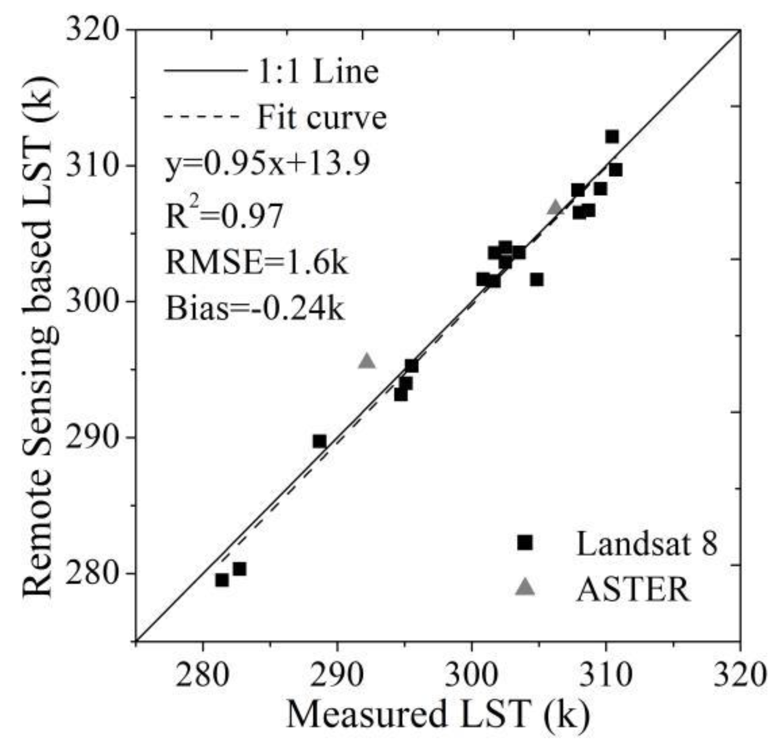
The surface temperature estimated from Landsat 8 and ASTER thermal infrared bands has a 30 m resolution and was compared with the site based radiometric temperature, as the underlying surface is flat and homogeneous. Figure 3 shows the comparison, and the determination coefficient (R2) between remote sensing derived and site observed surface temperatures was 0.97, yielding a mean absolute bias (bias) of −0.24 K, and a root mean square error (RMSE) of 1.6 K. The result indicated that although the remote sensing and site observations represent different spatial scales, the remote sensing-based radiometric surface temperature has reasonable accuracy.

4.2. Comparison of Estimated and Measured Instantaneous Surface Energy Fluxes

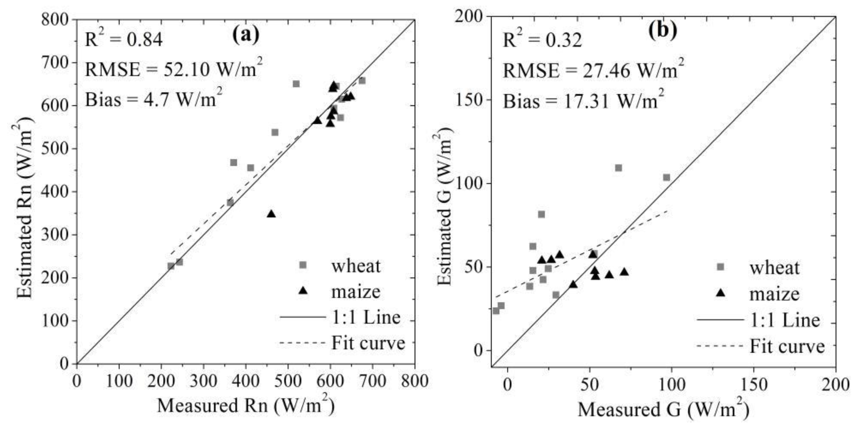
Remote sensing-based instantaneous net radiation yielded a root mean square error (RMSE) of 52.10 W/m2 and a bias of 4.7 W/m2; the R2 of 0.84 indicated that the evaluation of Rn had a high correlation with the site measurements (Figure 4a). The estimated instantaneous G was a little overestimated with a bias of 17.31 W/m2 and an RMSE of 27.46 W/m2. As shown in Figure 4b, the overestimation of the ground heat flux was more frequent during the winter wheat growing season; because the surface temperature always below or near the subsurface temperature in winter, the measured G may be negative or very low. However, as the proportion of G in the energy balance is the lowest, it does not cause much error in sensible and latent heat flux [26].
Figure 5 shows the comparisons of estimated and measured instantaneous LE for the three models. The correlations for estimated versus observed instantaneous LE values were different, with R2 values of 0.57, 0.78, and 0.66 for TSEB, 4s-PM, and PT-JPL models, respectively. The overall LE results from the 4s-PM model showed a stronger correlation than the other two models, which is different from some recent researches in the arid area [26]. In terms of LE error statistics, 4s-PM had the best performance with an RMSE of 84.63 W/m2 and a bias of 32.19 W/m2 in general. The RMSE values for PT-JPL and TSEB were close, but TSEB had the lowest bias of 28.99 W/m2. The PT-JPL showed an apparent underestimation for latent heat flux, with a Bias of −46.42 W/m2.
To further validate the results, the estimated instantaneous LE was compared for winter wheat and summer maize separately. Table 2 shows the statistics of the LE derived from the three models for summer maize and winter wheat. For the summer maize, the LE estimated from TSEB had the highest correction with the EC measurements, with an R2 of 0.9 and an RMSE of 75.0 W/m2. The results from 4s-PM showed an overestimation of LE for the maize and had the weakest performance among the three models. However, for the winter wheat, the 4s-PM estimated LE had the closest average value with the EC observation, with a high R2 value of 0.91 and an RMSE of 61.0 W/m2. On the contrary, the LE estimated from TSEB for wheat had the lowest correlation and the highest RMSE value.

4.3. Comparison of Spatially Distributed ET Flux

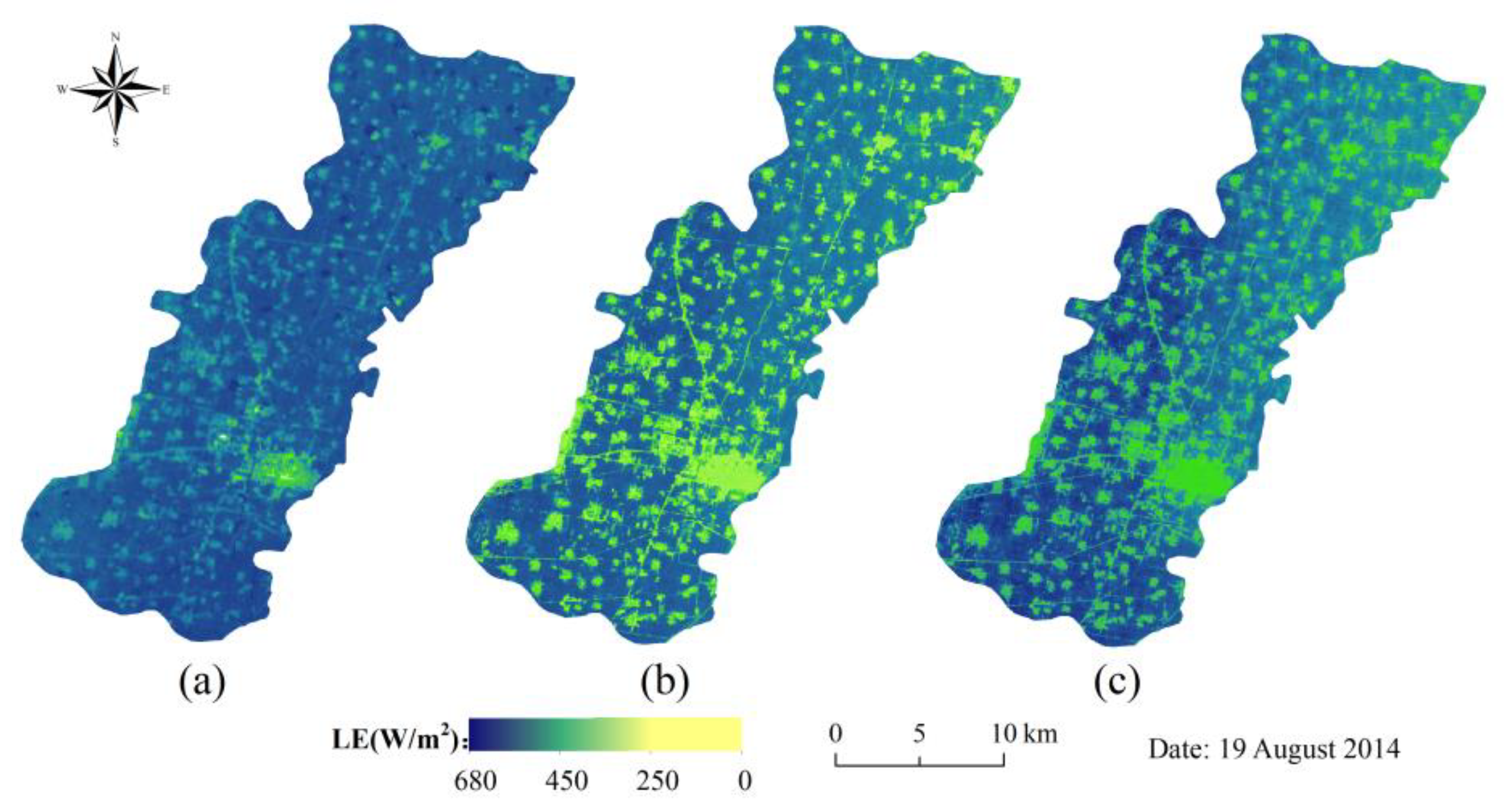
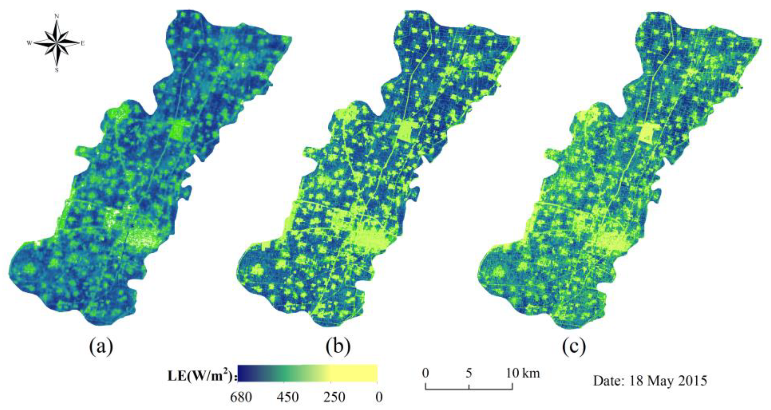
Figure 6 and Figure 7 show the spatial distribution of instantaneous latent heat flux during the summer maize (19 August 2014) and winter wheat (18 May 2015) growing seasons. Both the two days’ crops were flourishing with high NDVI values of 0.863–0.89; at this time, the latent heat exchange in the canopy was significant, and as a result, all the LE maps for the three models showed higher values for crop area, and lower values for the bare soil and artificial surface. Figure 8 shows the histogram of the LE maps over the summer maize area for the two days. On 19 August, the averaged LE values of all crop pixels for the 4s-PM and PT-JPL were close. The PT-JPL had the highest standard deviation; the LE values for the PT-JPL model had a broader range and mainly varied from 300 to 650 W/m2. The histograms’ shapes of 4s-PM and TSEB were more clustered, with pixel values ranging from 350 to 600 W/m2 for 4s-PM, and 450 to 600 W/m2 for TSEB. On 18 May, as shown in Figure 9, the pixels’ averaged LE values indicated an apparent underestimation of winter wheat ET for the PT-JPL model. The PT-JPL had the most significant standard deviation, which suggested that it had more capacity to exhibit crop ET heterogeneity. The 4s-PM and TSEB outputs had similar patterns and close average LE values for all winter wheat pixels.
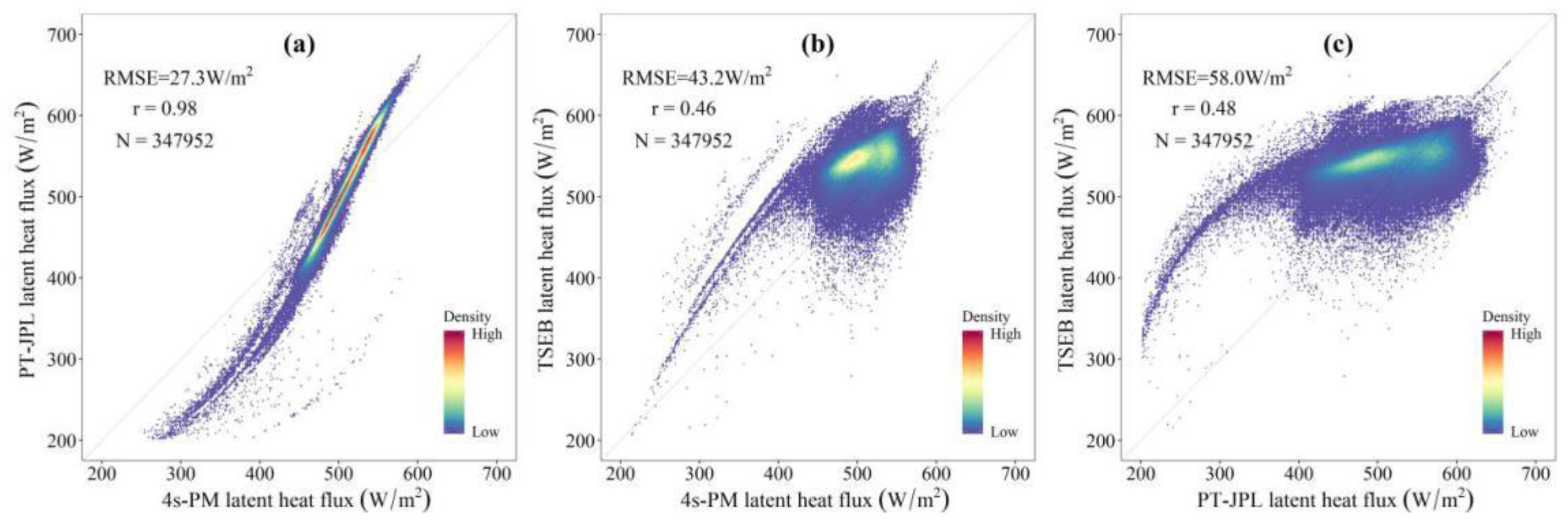
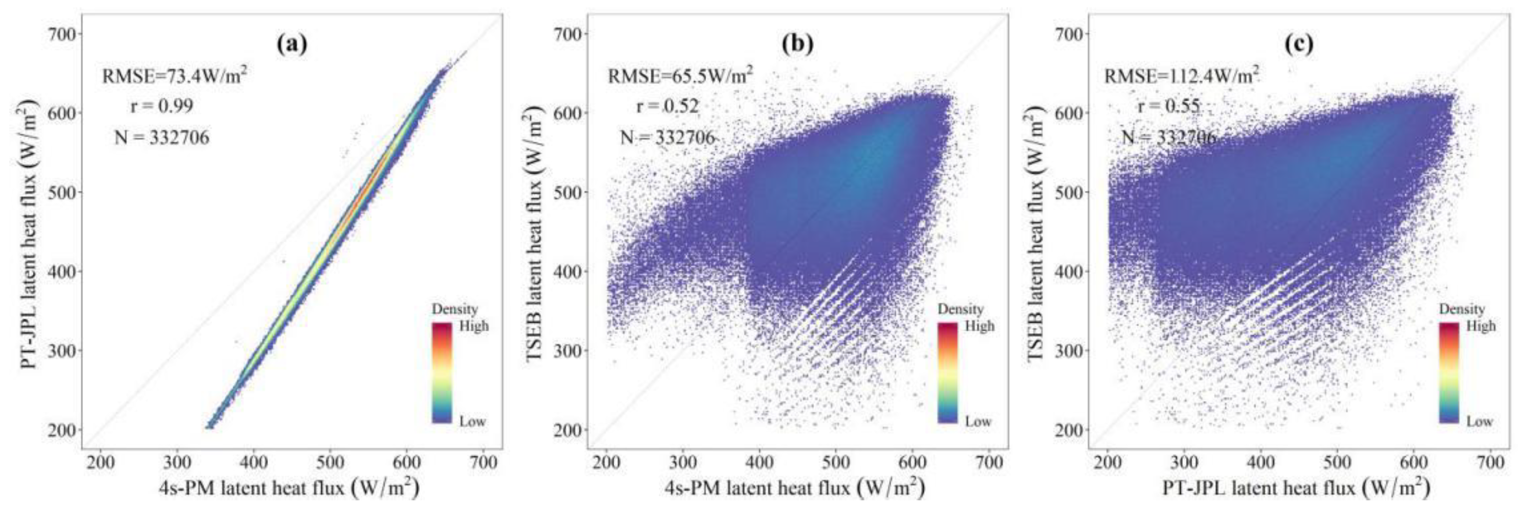
Figure 10 contains density plots of comparisons of maize instantaneous latent heat flux for the three models on 19 August 2014. The correlation coefficient (r) and root mean square error (RMSE) values were calculated from 347,952 pixels. Good agreement was obtained for the instantaneous LE derived from the 4s-PM and PT-JPL models, with r values equaling 0.98 and RMSE was 27.3 W/m2, while relatively weak agreement was obtained for LE estimations from 4s-PM, PT-JPL, and TSEB models (Figure 10b,c), with lower values for the correlation coefficient and higher RMSE. The most extensive density distribution of the estimated maize latent heat flux was ranged from 450 to 600 W/m2. In the range of 300 to 500 W/m2, the estimation of PT-JPL was lower than the result of 4s-PM, while in the range of 500 to 600 W/m2, it was the opposite. For the wheat (Figure 11), when growing at the most vigorous season on 18 May 2015, the estimations of 4s-PM and PT-JPL models exhibited a high degree of consistency, with a tremendous correlation coefficient value of 0.99. At the same time, most of the result for the 4s-PM model was higher than that of PT-JPL model in the whole wheat region. However, the comparisons of TSEB and the other two models, similar to maize, showed a lower correlation coefficient and higher RMSE values. The TSEB model estimation was generally higher than that of the PT-JPL model for the wheat.

5. Discussion

Although the three models were established with different assumptions and theories, they all provided relatively reliable estimates of ET. Many previous studies have shown that environmental factors, such as solar radiation, air temperature, air humidity, and soil moisture, may affect ET [15,32]. For the 4s-PM model, the canopy resistance is calculated using different environmental factors changes that control the leaf stoma opening and closing to increase or decrease the rate of evaporation under different environmental stresses. The PT-JPL model takes into account the influence of the optimum air temperature and humidity for vegetation evaporation. Although the TSEB model does not directly consider the influence of environmental stress factors, in its iterative solution process, the change of canopy and soil latent heat flux transfer mechanism caused by vegetation stress have been included. Under such a semi-humid region, the model’s feedback on environmental stress is different. In order to clarify this issue, Jarvis’s type [39,40] soil moisture (fsm), air humidity (fhu), air temperature (fta), and solar radiation (fsr) environmental factors were chosen to evaluate the model sensitivity. The fsm factor characterizes the role of soil moisture for canopy transpiration; the factor fhu also indicates water stress conditions, which is similar to fsm except from the air at the reference height. The fta factor incorporates air temperature constraints on canopy resistance, and it decreases when the air temperature at the reference height level above the canopy departs from the optimal temperature (e.g., 298 k) for the growth of many crops. The fsr factor is calculated from downward shortwave radiation, which implies the energy stress for heat flux [40]. All environmental factor values are between 0–1; lower values represent severer environmental stresses.
Table 3 shows the averaged values of different environmental factors for winter wheat and summer maize during the whole growing season, respectively. The winter wheat mainly grows from November to June of the following year, and the primary growing season of summer maize is from July to October. Table 3 indicates that the winter wheat suffered more from the soil moisture, air humidity, and air temperature stresses, as it grows in a much drier and colder season than the summer maize. However, the solar radiation stresses for wheat and maize were not obvious.
Table 4 and Table 5 show the environmental stress values and the three models’ estimation relative percentage errors for maize and wheat at different growth stages, respectively. For the two days at the early growth stage of maize, the fsm and fhu had approximate values, most likely because of irrigation; this indicated that the two factors both play a role in controlling water vapor exchange between canopy and atmosphere. Since none of the three models directly considered the effects of soil moisture, an overestimation of LE was found. Moreover, the PT-JPL considered the plant moisture stress, and the TSEB had an iteration of αpt decline under water-limited condition, the 4s-PM showed more significantly overestimated ET, with a higher relative error close to 50%. On 9 October, when the maize was at maturation stage, the cropland was also wet, since the fsm was about 0.57, the air humidity became the dominant factor with a lower value, and all the LE estimations of the three models showed an underestimation, especially for the PT-JPL model, with a relative error of −86%. At this growth stage, the leaves of crop lost vigor, and the reflectance in the near-infrared declined, leading to lower values of vegetation index and plant moisture stress; this is the reason that PT-JPL overestimated LE more obviously at this occasion.
In Table 5, at the early stage of wheat, the air temperature was very low; the TSEB model generated the most significant relative error of 34% for the lack of consideration of air temperature stress. At the middle stage of wheat, the crop was growing well with adequate water supply; the air humidity became the dominant stress factor. It indicated that the air humidity was inconsistent with soil moisture in this region. Both the PT-JPL and TSEB models underestimated LE obviously with relative errors ranged from −35%–−52%. At the maturation stage of wheat, apparent water stress was found on 13 June; moreover, the 4s-PM and TSEB models were unable to respond promptly to water deficit, leading to a more considerable overestimation of LE. However, the PT-JPL also underestimated LE as same as maize at the maturation growth stage for the uncertainty of plant moisture stress.
The comparison indicated that the soil moisture was a critical environmental factor in control of the water exchange from cropland and atmosphere, especially for the early and maturation growth stages for both wheat and maize in this region. The improved PT-JPL model had already incorporated spatially explicit daily surface soil moisture control on soil evaporation and canopy transpiration [44] at a global scale. However, this study did not introduce soil moisture data for evapotranspiration estimation. The primary reason was that the current spatial resolution of soil moisture remote sensing products still cannot meet the needs of evapotranspiration estimation at the field scale. The solar radiation factor had high values in different growing periods of both the two crops in this region, which meant that the energy supply had a weak effect on crop evapotranspiration. It is different from the findings in some natural drylands growing with perennial tussock grass, where both the soil moisture and energy supply actively reduce evapotranspiration obviously [38].

6. Conclusions

Remote sensing technology provides adequate data support for regional evapotranspiration estimation. In this paper, three mainstream multiple source ET models were tested using remote sensing data (Landsat 8 and ASTER) over cropland in a semi-humid region. The results of validation using tower observations demonstrated that the three models were capable of predicting relative reliable latent heat fluxes with different accuracies. Generally, the 4s-PM model had the best performance for both the wheat and maize and the PT-JPL and TSEB had the closest RMSE and determination coefficient values.
A further inter-comparison of the model results indicated that the latent heat flux of wheat estimated by the 4s-PM model had the highest accuracy with an RMSE of 61.0 W/m2 and an R2 of 0.91, and the TSEB performed well in estimating the latent heat flux of maize, with an RMSE of 75.0 W/m2 and an R2 of 0.9. The LE spatial distribution comparison indicated that the PT-JPL had the most significant standard deviation for all pixels, which meant that it had more capacity to exhibit crop evapotranspiration heterogeneity. Moreover, the density plots of all the LE pixels showed that the estimations of 4s-PM and PT-JPL were more relevant at the spatial scale.
Lastly, the model’s feedback on environmental stress was compared; the dominant environmental factors affecting evapotranspiration varied with crop types and crop growth stages. The wheat suffered more from the air temperature at its early growth stage. When both the soil moisture and air humidity were dominating factors at the early stage of maize, the three models all showed some overestimation of LE. Without considering soil moisture, 4s-PM and TSEB overestimated latent heat flux under water deficit in the maturation stage of wheat. The plant moisture stress calculated with the NDVI in PT-JPL underestimated the evaporation when the crop was in its maturation stage when the cropland was still wet. Although the soil moisture is essential in evapotranspiration estimation, the spatial resolutions’ insufficient of the soil moisture products limit the applications at the field scale.

Author Contributions

Q.Z. contributed to describing the models, put it into context, analyzed the results, prepared the figures and maps, and wrote the final manuscript. H.W. contributed to designing the experiment. Y.X. contributed to the remote sensing data, meteorological and EC data processing. All authors have read and agreed to the published version of the manuscript.

Funding

This research was funded by the National Key Research and Development Project (Grant No. 2017YFC0404503) and the Natural Science Foundation of the Jiangsu Higher Education Institutions of China (Grant No. 17KJB420002).

Acknowledgments

The authors are very thankful to Bingfang Wu and Jiaming Xu in the institute of remote sensing and digital earth, Chinese academy of sciences, for providing the meteorological data. The authors also thank Mingzhao Yu for providing the picture of the meteorological tower in Guantao.

Conflicts of Interest

The authors declare no conflict of interest.

References

  1. Merlin, O.; Chirouze, J.; Olioso, A.; Jarlan, L.; Chehbouni, G. An image-based four-source surface energy balance model to estimate crop evapotranspiration from solar reflectance/thermal emission data (SEB-4S). Agric. For. Meteorol. 2014, 184, 188–203. [Google Scholar] [CrossRef] [Green Version]
  2. Song, L.; Liu, S.; Kustas, W.P.; Zhou, J.; Xu, Z.; Xia, T.; Li, M. Application of remote sensing-based two-source energy balance model for mapping field surface fluxes with composite and component surface temperatures. Agric. For. Meteorol. 2016, 230-231, 8–19. [Google Scholar] [CrossRef] [Green Version]
  3. Norman, J.M.; Kustas, W.P.; Humes, K.S. Source approach for estimating soil and vegetation energy fluxes in observations of directional radiometric surface temperature. Agric. For. Meteorol. 1995, 77, 263–293. [Google Scholar] [CrossRef]
  4. Anderson, M.C.; Norman, J.M.; Mecikalski, J.R.; Otkin, J.A.; Kustas, W.P. A climatological study of evapotranspiration and moisture stress across the continental United States based on thermal remote sensing: 1. Model formulation. J. Geophys. Res. Atmos. 2007, 112. [Google Scholar] [CrossRef]
  5. Bastiaanssen, W.G.; Menenti, M.; Feddes, R.; Holtslag, A. A remote sensing surface energy balance algorithm for land (SEBAL). 1. Formulation. J. Hydrol. 1998, 212, 198–212. [Google Scholar] [CrossRef]
  6. Su, Z. The surface energy balance system (SEBS) for estimation of turbulent heat fluxes. Hydrol. Earth Syst. Sci. 2002, 6, 85–100. [Google Scholar] [CrossRef]
  7. Mu, Q.; Heinsch, F.A.; Zhao, M.; Running, S.W. Development of a global evapotranspiration algorithm based on modis and global meteorology data. Remote Sens. Environ. 2007, 111, 519–536. [Google Scholar] [CrossRef]
  8. Mu, Q.; Zhao, M.; Running, S.W. Improvements to a modis global terrestrial evapotranspiration algorithm. Remote Sens. Environ. 2011, 115, 1781–1800. [Google Scholar] [CrossRef]
  9. Xu, J.; Wu, B.; Yan, N.; Tan, S. Regional daily ET estimates based on the Gap-Filling Method of Surface Conductance. Remote Sens. 2018, 10, 554. [Google Scholar] [CrossRef] [Green Version]
  10. Zhuang, Q.; Wu, B.; Yan, N.; Zhu, W.; Xing, Q. A method for sensible heat flux model parameterization based on radiometric surface temperature and environmental factors without involving the parameter KB−1. Int. J. Appl. Earth Obs. Geoinf. 2016, 47, 50–59. [Google Scholar] [CrossRef]
  11. Paul, G.; Gowda, P.H.; Prasad, P.V.V.; Howell, T.A.; Aiken, R.M.; Neale, C.M.U. Investigating the influence of roughness length for heat transport (zoh) on the performance of SEBAL in semi-arid irrigated and dryland agricultural systems. J. Hydrol. 2014, 509, 231–244. [Google Scholar] [CrossRef]
  12. Boulet, G.; Olioso, A.; Ceschia, E.; Marloie, O.; Coudert, B.; Rivalland, V.; Chirouze, J.; Chehbouni, G. An empirical expression to relate aerodynamic and surface temperatures for use within single-source energy balance models. Agric. For. Meteorol. 2012, 161, 148–155. [Google Scholar] [CrossRef] [Green Version]
  13. Mallick, K.; Jarvis, A.J.; Boegh, E.; Fisher, J.B.; Drewry, D.T.; Tu, K.P.; Hook, S.J.; Hulley, G.; Ardö, J.; Beringer, J.; et al. A surface Temperature Initiated Closure (STIC) for surface energy balance fluxes. Remote Sens. Environ. 2014, 141, 243–261. [Google Scholar] [CrossRef]
  14. Nishan Bhattarai, N.; Mallick, K.; Brunsell, N.A.; Sun, G.; Jain, M. Regional evapotranspiration from an image-based implementation of the Surface Temperature Initiated Closure (STIC1.2) model and its validation across an aridity gradient in the conterminous US. Hydrol. Earth Syst. Sci. 2018, 22, 2311–2341. [Google Scholar] [CrossRef] [Green Version]
  15. Gokmen, M.; Vekerdy, Z.; Verhoef, A.; Verhoef, W.; Batelaan, O.; van der Tol, C. Integration of soil moisture in SEBS for improving evapotranspiration estimation under water stress conditions. Remote Sens. Environ. 2012, 121, 261–274. [Google Scholar] [CrossRef]
  16. Yang, Y.; Qiu, J.; Zhang, R.; Huang, S.; Chen, S.; Wang, H.; Luo, J.; Fan, Y. Intercomparison of Three Two-Source Energy Balance Models for Partitioning Evaporation and Transpiration in Semiarid Climates. Remote Sens. 2018, 10, 1149. [Google Scholar] [CrossRef] [Green Version]
  17. Zhuang, Q.; Wu, B. Estimating Evapotranspiration from an Improved Two-Source Energy Balance Model Using ASTER Satellite Imagery. Water 2015, 7, 6673–6688. [Google Scholar] [CrossRef] [Green Version]
  18. Norman, J.M.; Kustas, W.P.; Prueger, J.H.; Diak, G.R. Surface flux estimation using radiometric temperature: A dual-temperature-difference method to minimize measurement errors. Water Resour. Res. 2000, 36, 1898–1908. [Google Scholar] [CrossRef] [Green Version]
  19. Fisher, J.B.; Tu, K.P.; Baldocchi, D.D. Global estimates of the land–atmosphere water flux based on monthly AVHRR and ISLSCP-II data, validated at 16 FLUXNET sites. Remote Sens. Environ. 2008, 112, 901–919. [Google Scholar] [CrossRef]
  20. Garcia, M.; Sandholt, I.; Ceccato, P.; Ridler, M.; Mougin, E.; Kergoat, L.; Morillsa, L.; Timouk, F.; Fensholt, R.; Domingo, F. Actual evapotranspiration in drylands derived from in situ and satellite data: Assessing biophysical constraints. Remote Sens. Environ. 2013, 131, 103–118. [Google Scholar] [CrossRef]
  21. Yilmaz, M.T.; Anderson, M.C.; Zaitchik, B.; Hain, C.R.; Crow, W.T.; Ozdogan, M.; Chun, J.A.; Evans, J. Comparison of prognostic and diagnostic surface flux modeling approaches over the nile river basin. Water Resour. Res. 2014, 50, 386–408. [Google Scholar] [CrossRef]
  22. Yan, H.; Wang, S.; Billesbach, D.; Oechel, W.; Zhang, J.; Meyers, T.; Martin, T.; Matamala, R.; Baldocchi, D.; Bohrer, G.; et al. Global estimation of evapotranspiration using a leaf area index-based surface energy and water balance model. Remote Sens. Environ. 2012, 124, 581–595. [Google Scholar] [CrossRef] [Green Version]
  23. Bai, Y.; Zhang, J.; Zhang, S.; Koju, U.A.; Yao, F.; Igbawual, T. Using precipitation, vertical root distribution, and satellite-retrieved vegetation information to parameterize water stress in a Penman-Monteith approach to evapotranspiration modeling under Mediterranean climate. J. Adv. Model. Earth Syst. 2017, 9, 168–192. [Google Scholar] [CrossRef]
  24. Bai, Y.; Zhang, J.; Zhang, S.; Yao, F.; Magliuloc, V. A remote sensing-based two-leaf canopy conductance model: Global optimization and applications in modeling gross primary productivity and evapotranspiration of crops. Remote Sens. Environ. 2018, 215, 411–437. [Google Scholar] [CrossRef]
  25. Lian, J.; Huang, M. Comparison of three remote sensing based models to estimate evapotranspiration in an oasis-desert region. Agric. For. Meteorol. 2016, 165, 153–162. [Google Scholar] [CrossRef]
  26. Yang, Y.; Long, D.; Guan, H.; Liang, W.; Simmons, C.; Batelaan, O. Comparison of three dual-source remote sensing evapotranspiration models during the MUSOEXE-12 campaign: Revisit of model physics. Water Resour. Res. 2015, 51, 3145–3165. [Google Scholar] [CrossRef]
  27. Xu, E.; Wang, R.; Zhang, H.; Yu, Z. Coupling index of water consumption and soil fertility correlated with winter wheat production in North China Region. Ecol. Indic. 2019, 102, 154–165. [Google Scholar] [CrossRef]
  28. Sun, H.; Zhang, X.; Liu, X.; Liu, X.; Shao, L.; Chen, S.; Wang, J.; Dong, X. Impact of different cropping systems and irrigation schedules on evapotranspiration, grain yield and groundwater level in the North China Plain. Agric. Water Manag. 2019, 19, 202–209. [Google Scholar] [CrossRef]
  29. Yang, Y.; Luo, Y.; Wu, C.; Zheng, H.; Zhang, L.; Cui, Y.; Sun, N.; Wang, L. Evaluation of six equations for daily reference evapotranspiration estimating using public weather forecast message for different climate regions across China. Agric. Water Manag. 2019, 222, 386–399. [Google Scholar] [CrossRef]
  30. Fang, B.; Lei, H.; Zhang, Y.; Quan, Q.; Yang, D. Spatio-temporal patterns of evapotranspiration based on upscaling eddy covariance measurements in the dryland of the North China Plain. Agric. For. Meteorol. 2020, 281, 107844. [Google Scholar] [CrossRef]
  31. Wang, Q.; Tang, J.; Zeng, J.; Qu, Y.; Zhang, Q.; Shui, W.; Wang, W.; Yi, L.; Leng, S. Spatial-temporal evolution of vegetation evapotranspiration in Hebei Province, China. J. Integr. Agric. 2018, 17, 2107–2117. [Google Scholar] [CrossRef] [Green Version]
  32. Yu, M.; Wu, B.; Yan, N.; Xing, Q.; Zhu, W. A Method for Estimating the Aerodynamic Roughness Length with NDVI and BRDF Signatures Using Multi-Temporal Proba-V Data. Remote Sens. 2017, 9, 6. [Google Scholar] [CrossRef] [Green Version]
  33. Twine, T.E.; Kustas, W.P.; Norman, J.M.; Cook, D.R.; Houser, P.R.; Meyers, T.P.; Prueger, J.H.; Starks, P.J.; Wesely, M.L. Correcting eddy-covariance flux underestimates over a grassland. Agric. For. Meteorol. 2000, 103, 279–300. [Google Scholar] [CrossRef] [Green Version]
  34. Liang, S. Narrowband to broadband conversions of land surface albedo. I Algorithms. Remote Sens. Environ. 2001, 76, 213–238. [Google Scholar] [CrossRef]
  35. Sobrino, J.A.; Jiménez-Muñoz, J.C.; El-Kharraz, J.; Gómez, M.; Romaguera, M.; Sòria, G. Single-channel and two channel methods for land surface temperature retrieval from DAIS data and its application to the Barrax site. Int. J. Rem. Sens. 2004, 25, 215–230. [Google Scholar] [CrossRef]
  36. Kustas, W.P.; Norman, J.M. Evaluation of soil and vegetation heat flux predictions using a simple two-source model with radiometric temperatures for partial canopy cover. Agric. For. Meteorol. 1999, 94, 13–29. [Google Scholar] [CrossRef]
  37. Allen, R.G.; Tasumi, M.; Trezza, R. Satellite-based energy balance for mapping evapotranspiration with internalized calibration (METRIC)-model. J. Irrig. Drain. Eng. 2007, 133, 380–394. [Google Scholar] [CrossRef]
  38. Morillas, L.M.; Villagarcia, L.; Domingo, F.; Nieto, H.; Ucles, O.; Garcia, M. Environmental factors affecting the accuracy of surface fluxes from a two-source model in Mediterranean drylands: Upscaling instantaneous to daytime estimates. Agric. For. Meteorol. 2014, 189–190, 140–158. [Google Scholar] [CrossRef]
  39. Jarvis, P. The interpretation of the variations in leaf water potential and stomatal conductance found in canopies in the field. Philos. Trans. R. Soc. Lond. B 1976, 273, 593–610. [Google Scholar]
  40. Chen, F.; Dudhia, J. Coupling an advanced land surface-hydrology model with the Penn State-NCAR MM5 modeling system. Part 1: Model implementation and sensitivity. Mon. Weather Rev. 2001, 129, 569–585. [Google Scholar] [CrossRef] [Green Version]
  41. Ghilain, N.; Arboleda, A.; Gellens-Meulenberghs, F. Evapotranspiration modelling at large scale using near-real time MSG SEVIRI derived data. Hydrol. Earth Syst. Sci. 2011, 15, 771–786. [Google Scholar] [CrossRef] [Green Version]
  42. Cui, Y.; Jia, L. A Modified Gash Model for Estimating Rainfall Interception Loss of Forest Using Remote Sensing Observations at Regional Scale. Water 2014, 6, 993–1012. [Google Scholar] [CrossRef] [Green Version]
  43. Masria, B.E.; Rahmanb, A.F.; Dragoni, D. Evaluating a new algorithm for satellite-based evapotranspiration for North American ecosystems: Model development and validation. Agric. For. Meteorol. 2019, 268, 234–248. [Google Scholar] [CrossRef]
  44. Purdy, A.J.; Fisher, J.B.; Goulden, M.L.; Colliander, A.; Halverson, G.; Tu, K.; Famiglietti, J.S. Smap soil moisture improves global evapotranspiration. Remote Sens. Environ. 2018, 219, 1–14. [Google Scholar] [CrossRef]
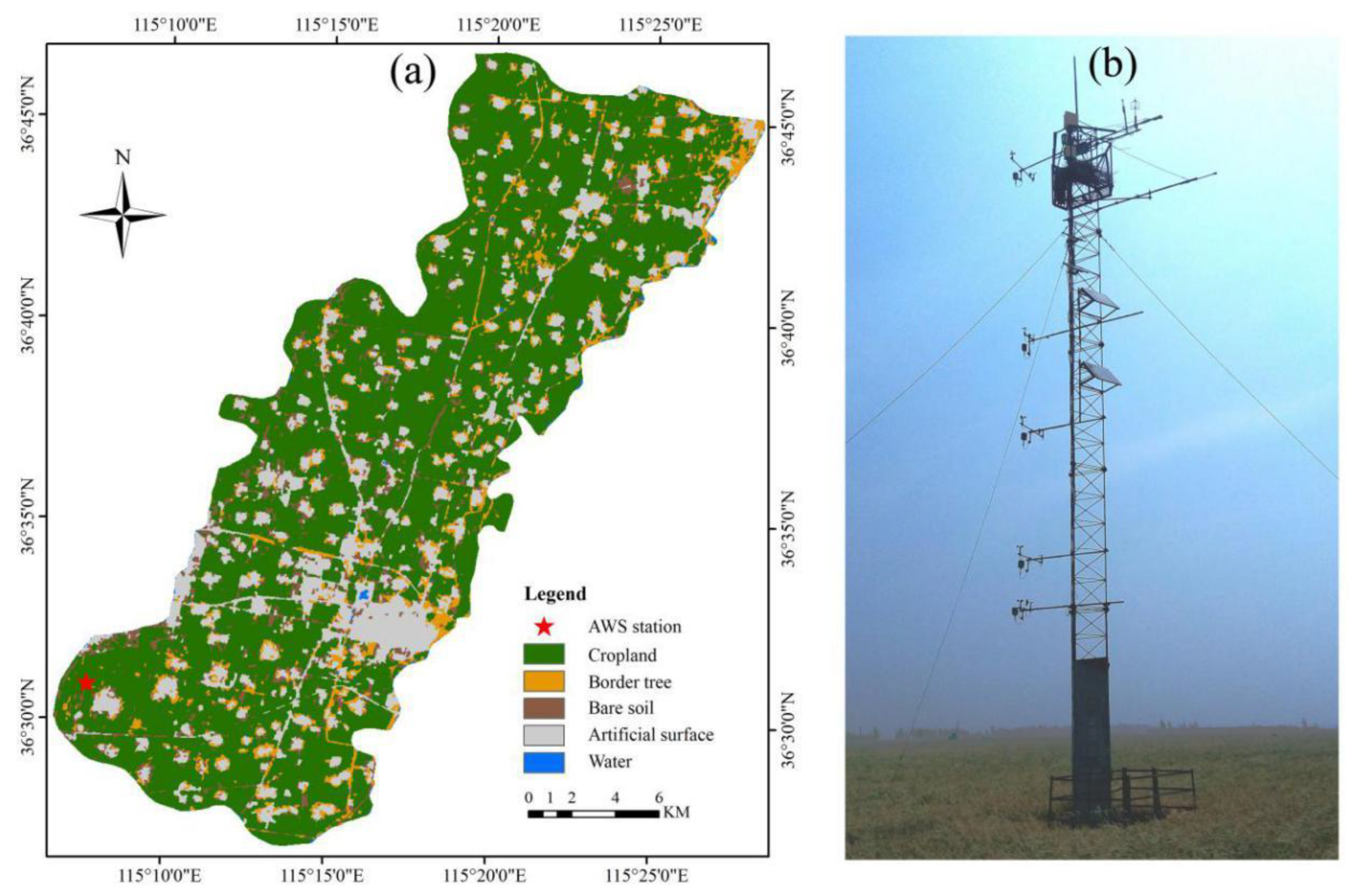
Figure 1. (a) Land cover map of Guantao County in 2014; (b) The photograph of the AWS and EC tower in Guantao during the winter wheat growing season.
Atmosphere 11 00325 g001
Figure 2. (a) EC measured hourly surface energy fluxes on 18 May 2015; (b) Surface energy balance closure from EC measurements at 11.00 a.m. in 2013–2017.
Atmosphere 11 00325 g002
Figure 3. Scatterplot of the remote sensing-based LST versus the surface temperatures measured by the infrared thermometers at the site.
Atmosphere 11 00325 g003
Figure 4. Validation of the measured and estimated Rn (a) and G (b) at the Guantao site.
Atmosphere 11 00325 g004
Figure 5. Validation of the instantaneous LE for different modes: (a) TSEB, (b) 4s-PM, and (c) PT-JPL.
Atmosphere 11 00325 g005
Figure 6. Spatial distribution of instantaneous summer maize LE derived from Landsat 8 on 19 August of 2014 for the (a) TSEB, (b) 4s-PM, and (c) PT-JPL models.
Atmosphere 11 00325 g006
Figure 7. Spatial distribution of instantaneous winter wheat LE derived from Landsat 8 on 18 May 2015 for the (Equation) TSEB, (Equation) 4s-PM, and (Equation) PT-JPL models.
Atmosphere 11 00325 g007
Figure 8. Histogram of the LE on 19 August of 2014 for different modes: (a) TSEB, (b) 4s-PM, and (c) PT-JPL.
Atmosphere 11 00325 g008
Figure 9. Histogram of the LE on 18 May of 2015 for different modes: (a) TSEB, (b) 4s-PM, and (c) PT-JPL.
Atmosphere 11 00325 g009
Figure 10. Density plots of comparisons of maize instantaneous latent heat flux derived from Landsat 8 for the three models ((a) 4s-PM vs. PT-JPL, (b) 4s-PM vs. TSEB, (c) PT-JPL vs. TSEB) on 19 August of 2014. The legend refers to the frequency of data points at each location.
Atmosphere 11 00325 g010
Figure 11. Density plots of comparisons of wheat instantaneous latent heat flux derived from Landsat 8 for the three models ((a) 4s-PM vs. PT-JPL, (b) 4s-PM vs. TSEB, (c) PT-JPL vs. TSEB) on 18 May of 2015. The legend refers to the frequency of data points at each location.
Atmosphere 11 00325 g011
Table 1. The image acquisition dates of Landsat 8 and ASTER and the provided data.
SensorDateProvided Data
Landsat 813 June 2013, 31 July 2013, 1 September 2013, 18 July 2014,
19 August 2014, 4 September 2014, 25 December 2014, 15 March 2015, 18 May 2015, 19 June 2015, 9 October 2015, 13 January 2016,
1 March 2016, 18 April 2016, 4 May 2016, 21 June 2016,
9 September 2016, 21 April 2017, 10 July 2017
(i)Radiance in visible and near infrared bands
(ii)Thermal infrared radiance in Band 10
ASTER6 July 2014, 25 March 2014(i) ASTER L2 surface reflectance VNIR V003
(ii) ASTER L2 surface temperature V003
Table 2. Statistics of the three models derived Latent heat flux for maize and wheat.
CropObserved Averaged (W/m2)TSEB4s-PMPT-JPL
Estimated Averaged (W/m2)RMSE (W/m2)R2Estimated Averaged (W/m2)RMSE (W/m2)R2Estimated Averaged (W/m2)RMSE (W/m2)R2
Maize361.8419.375.00.90441.9108.40.74374.791.00.68
Wheat280.6 288.2127.80.53276.861.00.91189.7118.60.88
Table 3. Mean environmental stress values for maize and wheat.
Crop TypeMean Environmental Stress
fsmfhuftafsr
Summer maize0.770.560.980.98
Winter wheat0.670.470.720.97
Table 4. Environmental stress and LE estimation relative percentage errors for maize.
DateGrowth StageEnvironmental StressMultipleRelative Error (100%)
fsmfhuftafsrTSEB4s-PMPT-JPL
31 July 2013Early0.860.750.960.980.600.260.470.32
18 July 20140.780.740.970.980.550.290.520.37
1 September 2013Middle0.610.451.000.980.270.000.22−0.17
9 October 2015Maturation0.570.190.970.960.10−0.21−0.13−0.86
Table 5. Environmental stress and LE estimation relative percentage errors for wheat.
DateGrowth StageEnvironmental StressMultipleRelative Error (100%)
fsmfhuftafsrTSEB4s-PMPT-JPL
13 January 2016Early0.500.510.010.900.010.34−0.15−0.19
18 April 2016Middle0.940.330.870.990.26−0.35−0.24−0.51
21 April 20170.890.400.890.990.32−0.520.03−0.41
13 June 2013Maturation0.250.390.990.990.091.500.57−0.50