Precipitation Nowcasting with Orographic Enhanced Stacked Generalization: Improving Deep Learning Predictions on Extreme Events

Abstract

One of the most crucial applications of radar-based precipitation nowcasting systems is the short-term forecast of extreme rainfall events such as flash floods and severe thunderstorms. While deep learning nowcasting models have recently shown to provide better overall skill than traditional echo extrapolation models, they suffer from conditional bias, sometimes reporting lower skill on extreme rain rates compared to Lagrangian persistence, due to excessive prediction smoothing. This work presents a novel method to improve deep learning prediction skills in particular for extreme rainfall regimes. The solution is based on model stacking, where a convolutional neural network is trained to combine an ensemble of deep learning models with orographic features, doubling the prediction skills with respect to the ensemble members and their average on extreme rain rates, and outperforming them on all rain regimes. The proposed architecture was applied on the recently released TAASRAD19 radar dataset: the initial ensemble was built by training four models with the same TrajGRU architecture over different rainfall thresholds on the first six years of the dataset, while the following three years of data were used for the stacked model. The stacked model can reach the same skill of Lagrangian persistence on extreme rain rates while retaining superior performance on lower rain regimes.

1. Introduction

Nowcasting—i.e., short-term prediction up to 6 h—of precipitation is a crucial tool for risk mitigation of water-related hazards [1,2,3,4,5]. The use of extrapolation methods on weather radar reflectivity sequences is the mainstay of very short-time (up to 2 h) precipitation nowcasting systems [6]. The raw reflectivity volume generated at fixed time steps by the radar is usually corrected by spurious echoes and processed into one or more products. In the case of a network of multiple radars, several strategies are used to merge the resulting volumes or products and generate a composite map. The most common products used as input to nowcasting models are reflectivity maps at constant altitude, such as Plain Positions Indicators (PPI) or Constant Altitude Plain Position Indicator (CAPPI), or the Maximum vertical reflectivity (CMAX or MAX(Z)). Sequences of reflectivity maps are used as input for prediction models. More formally, given a reflectivity field at time $T_0$, radar-based nowcasting methods aim to extrapolate m future time steps $T_1,T_2,\dots ,T_m$ in the sequence, using as input the current and n previous observations $T_{-n},\dots ,T_{-1},T_0$.

Traditional nowcasting models are manly based on Lagrangian echo extrapolation [7,8], with recent modification that try to infer precipitation growth and decay [9,10] or integrate with Numerical Weather Predictions to extend the time horizon of the prediction [11,12]. In the last few years, Deep Learning (DL) models based on combination of Recurrent Neural Networks (RNN) and Convolutional Neural Networks (CNN) have shown substantial improvement over nowcasting methods based on Lagrangian extrapolations for quantitative precipitation forecasting (QPF) [13]. Shi et al. [14] introduced the application of the Convolutional Long Short-Term Memory (Conv-LSTM) network architecture with the specific goal of improving precipitation nowcasting over extrapolation models, where LSTM is modified using a convolution operator in the state-to-state and input-to-state transitions. Subsequent work introduced dynamic recurrent connections [15] (TrajGRU) that allowed the improvement of prediction skills, spatial resolution, and temporal length of the forecast, with comparable number of parameters and memory requirements. Subsequent works introduced more complex memory blocks and architectures [16] and increased number of connections among layers [17,18] to further improve prediction skills at the expenses of an increase in computational complexity and memory requirements. Approaches based on pure CNN architectures have also been presented [19,20], showing how simple models can deliver better skills over traditional extrapolation on low to medium rain rates. Recently, prediction of multi-channel radar products simultaneously [21] has been explored, too.

While deep learning models have shown to consistently deliver superior forecast skills for the prediction of low to medium rain thresholds, few studies consider the case of extreme rain rates, where Lagrangian-based extrapolation methods can sometimes deliver better scores for short lived precipitation patterns, due to their heavy reliance on persistence. In fact, the main challenge faced by nowcasting methods is the progressive accumulation of uncertainty: DL architectures deal with uncertainty by smoothing prediction over time, using the intrinsic averaging effect of loss functions such as Mean Squared Error (MSE) and Mean Absolute Error (MAE), commonly used as loss functions to train DL architectures in regression problems [22]. This smoothing problem can be seen as Conditional Bias (CB): the minimization of MSE leads to models where peak values are systematically underestimated and compensated by overestimation in weak rain-rates [9,23]. Moreover, the minimization of these two errors is at odds [24]: measures taken to remove CB lead to an increase in MSE, and vice versa, the minimization of MSE results in a higher CB, manifested in an underestimation of high and extreme rain rates.

While not addressing the problem directly, some DL approaches try to cope with CB by introducing weighted loss functions [15], by integrating loss functions used in computer vision [25], or by optimizing for specific rain regimes [26]. Others avoid the problem by renouncing to a fully quantitative prediction and threshold the precipitation at specific rain-rates, approaching the nowcasting as a classification problem [20,27]. Unfortunately, while applying modification on the loss function can result in improvement for the general case, the current knowledge on loss functions suggests that this approach alone cannot be used to improve predictions of extreme events [28].

Instead of solely relying on loss function, in this work, we improve the prediction skills of deep learning models, especially for extreme rain rates, by combining orographic features with a model ensemble. Ensemble models are extensively used in meteorology for improving predictions skills, to estimate prediction uncertainty, or to generate probabilistic forecasts [29]. Despite their potential, the use of ensembles is problematic for deterministic nowcasting, because model averaging exacerbates the CB problem, leading to attenuation on extreme rain rates [30]. Thus, we use model stacking [31,32], where the outputs of a deep learning ensemble and orographic features are combined by another DL model to enhance the skill of existing predictions.

The paper is structured as follows. In Section 2, we introduce all the components of our solution, namely the dataset (Section 2.1), the DL nowcasting model used to create the ensemble (Section 2.2), the ensemble generation strategy (Section 2.3), the Stacked Generalization model (Section 2.4) with the Orographic Feature Enhancements (Section 2.5), and the Extrapolation Model used for the comparison (Section 2.6). This is followed by the presentation of the results in Section 3. Results are discussed in Section 4, followed by the summary and conclusions in Section 5.

2. Materials and Methods

2.1. TAASRAD19 Dataset

The dataset for this study was provided by Meteotrentino, the public weather forecasting service of the Civil Protection Agency of the Autonomous Trentino Province in Italy. The agency operates a weather radar located in the middle of the Italian Alps, on Mt. Macaion (1866 m.a.s.l.). The C-Band radar operates with a 5-min frequency for a total of 288 scans per day, and the generated products cover a diameter of 240 km at 500 m resolution, represented as a 480 × 480 floating point matrix. The publicly released TAASRAD19 [33,34] dataset consists of a curated selection of the MAX(Z) product of the radar in ASCII grid format, spanning from June 2010 to November 2019 for a total of 894,916 scans. The maximum reflectivity value reported by the product is $52.5$ dBZ, corresponding to 70 mm/h when converted to rain rate using the Z–R relationship developed by Marshall and Palmer [6] ($Z=200R^{1.6}$). An example of scan is reported in Figure 1.

For the purpose of this study, we split the data by day and grouped the radar scans into chunks of contiguous frames, generating chunks of at least 25 frames (longer than 2 h) and with a maximum length of 288 frames (corresponding to the whole day). Only chunks with precipitation are kept. Then, we divided the data into two parts: the first period from June 2010 to December 2016 was used to train and validate the model ensemble (TRE), while the precipitation events from January 2017 to July 2019 were used to generate the ensemble predictions. These were in turn used to train, validate, and test the stacked model (ConvSG). During the last stage, we also tested the integration of orographic features in the model chain. Figure 2 summarizes the overall flow of the data architecture used in the study.

2.2. Deep Learning Trajectory GRU Model

We adopt the trajectory gated recurrent unit (TrajGRU) network structure proposed by Shi et al. in [15] as baseline model to build our ensemble. We note that a single instance of this model has already been integrated internally to the Civil Protection for nowcasting assessments. The underlying idea of the model is to use convolutional operations in the transitions between RNN cells instead of fully connected operations to capture both temporal and spatial correlations in the data. Moreover, the network architecture dynamically determines the recurrent connections between current input and previous state by computing the optical flow between feature maps, both improving the ability to describe spatial relations and reducing the overall number of operations to compute. The network is designed using an encoder–forecaster structure in three layers: in the encoders, the feature maps are extracted and down-sampled to be fed to the next layer, while the decoder connects the layers in the opposite direction, using deconvolution to up-sample the features and build the prediction. With this arrangement, the network structure can be modified to support an arbitrary number of input and output frames. In our configuration, 5 frames (25 min) are used as input to predict the next 20 steps (100 min), at the full resolution of the radar (480 × 480 pixels). Figure 3 shows the model architecture diagram.

Given the complex orographic environment where the radar operates, the data products suffer from artifacts and spurious signals even after the application of the polar filter correction. For this reason, we generate a static mask (MASK) using the procedure adopted in [15]: the mask is used to systematically exclude out of distribution pixels when computing the loss function during training. As loss function, we adopt the same weighted combination of MAE and MSE proposed by Shi et al. [15], where target pixels with higher rain rate are multiplied by a higher weight, while for masked pixels the weight is set to zero. Specifically, given a pixel x, the weight $w(x)$ is computed as the stepwise function $w(x)$ proposed by [15]:

$$w(x)=\left\{\begin{array}{cc}0\hfill & \mathrm{if}xϵ\mathrm{MASK}\hfill \\ 1\hfill & \mathrm{if}R(x)<2\hfill \\ 2\hfill & \mathrm{if}2\le R(x)<5\hfill \\ 5\hfill & \mathrm{if}5\le R(x)<10\hfill \\ 10\hfill & \mathrm{if}10\le R(x)<30\hfill \\ 30\hfill & \mathrm{if}R(x)\ge 30,\hfill \end{array}\right.$$

(1)

where $R(x)$ is the Z-R Marshall Palmer conversion with the parameters described in Section 2.1. The final loss equation is given by the sum of the weighted errors

$$\mathrm{B}-\mathrm{MAE}+\mathrm{B}-\mathrm{MSE}=\frac{1}{N}\sum _{n=1}^N\sum _{i=1}^{480}\sum _{j=1}^{480}{w}_{nij}{(x_{nij}-{\tilde{x}}_{nij})}^2+\frac{1}{N}\sum _{n=1}^N\sum _{i=1}^{480}\sum _{j=1}^{480}{w}_{nij}|x_{nij}-{\tilde{x}}_{nij}|,$$

(2)

where w are the weights, x is the observation, $\tilde{x}$ is the prediction, and N is the number of frames. This loss function gives the flexibility to fine-tune the training process by forcing the network to focus on specific rain regimes at the pixel level, thus already mitigating CB, with a concept that reminds spatial attention layers [35]. Augmenting the loss with functions considering also neighbor pixels (e.g., SSIM [25]) is not feasible here: indeed, the spatial incongruities introduced by pixel masking and the circular (non-rectangular) output of the prediction target require using a loss function operating at single-pixel level.

2.3. Thresholded Rainfall Ensemble for Deep Learning

We base our ensemble on different realizations of the TrajGRU model, given its strength and flexibility for the task. Ideally, a reliable ensemble should be able to sample the complete underlying distribution of the phenomenon [36]. For precipitation nowcasting, the ensemble should be able to fully cover the different precipitation scenarios into which the input conditions can develop. For extreme precipitations, we aim to model the variability of the boundary conditions that can lead to an extreme event by generating an ensemble that can mimic the different scenarios. There are two common approaches for building an ensemble from a single DL model: either adding random perturbations to the initial conditions of the model or training the model on a different subset of the input space, e.g., via bagging [37]. Our solution differs from these approaches and it uses the mechanism described in Section 2.2 to modify the loss weights of lower rain rate pixels. Specifically, the weight for pixels under a certain threshold is set by modifying the computation of the loss as follows:

$$w\left(x\right)=\left\{\begin{array}{cc}0\hfill & \mathrm{if}\left(xϵ\mathrm{MASK}\right)\wedge \left(R\right(x)<\mathrm{T})\hfill \\ 1\hfill & \mathrm{if}\mathrm{T}\le R\left(x\right)<2\hfill \\ 2\hfill & \mathrm{if}2\le R\left(x\right)<5\hfill \\ 5\hfill & \mathrm{if}5\le R\left(x\right)<10\hfill \\ 10\hfill & \mathrm{if}10\le R\left(x\right)<30\hfill \\ 30\hfill & \mathrm{if}R\left(x\right)\ge 30,\hfill \end{array}\right.$$

(3)

where T is a threshold value in the set T $ϵ\{0.03,0.06,0.1,0.3\}$, thus building an ensemble of 4 models. With this approach, the model does not need to optimize for all precipitation regimes under the threshold during training and considers as an optimization target only the higher rain rates. The mechanism produces a progressive overshooting of the total amount of rain estimate when rising the threshold, which in turn helps target higher rain regimes. Figure 4 shows the progressive rise in the average pixel value of the generated predictions of the 4 models on the test set.

We call this approach thresholded rainfall ensemble (TRE). TRE has several desirable properties: it does not require any sampling of the input data, and it is able to generate models with significantly different behaviors using a single model architecture. Moreover, all the ensemble members in TRE keep as primary objective in the loss function the minimization of the error on the high rain rates. Finally, TRE allows tuning the ensemble spread by choosing a more similar or more distant set of thresholds, a property that is not achievable with random data re-sampling or via random parameterization. The only drawback of this method is that the choice of thresholds is dependent on the distribution of the dataset, and thus the generated spread can only be empirically tested. However, the presented thresholds can be reused as is at least on other Alpine radars, and with minor modifications in continental areas. Indeed, the thresholds are considered on the actual rainfall rate calculated after the conversion from reflectivity, where all variability given from the physical characteristics of the radar, background noise, and environmental factors have already been taken into account and corrected.

An example of the prediction behavior of the four models is shown in Figure 5, along with the input and observed precipitation.

As introduced in Figure 2, the four models composing the TRE ensemble were trained on the TAASRAD19 data from 2010 to 2016. Using a moving window of 25 frames on the data chunks, we extracted all the sequences with precipitation in the period, for a total of $\mathrm{202,054}$ sequences: $95\%$ ($\mathrm{191,952}$) were used for training while $5\%$ ($\mathrm{10,102}$) were reserved for validation and model selection. All models were trained with the same parameters except for the threshold: fixed random seed, batch size 4, Adam optimizer [38] with learning rate ${10}^{-4}$ and learning rate decay, 100,000 training iterations with model checkpoint, and validation every 10,000 iteration. For each threshold value, the model with the lowest validation loss was selected as a member of the ensemble.

2.4. ConvSG Stacking Model

Stacked Generalization (or model stacking) is a strategy that employs the predictions of an ensemble of learners to train a model on top of the ensemble predictions, with the goal of improving the overall accuracy. The objective of our stacking model is to combine the ensemble outputs to reduce CB in the prediction.

We first generate the stacked model training set, i.e., the predictions for each ensemble member for the data for 2017–2019, for a total of $\mathrm{76,151}\times 4$ set of prediction sequences, where each sequence is a tensor of size $20\times 480\times 480$. Given that extreme precipitations are very localized in space and time, we need to preserve both the spatial an temporal resolution of the prediction. Since the theoretical input size for the stacked model results in a tensor of size $4\times 20\times 480\times 480$, memory and computing resources are to be carefully planned. To avoid hitting the computational wall, we developed a stacking strategy based on the processing of a stack of the first predicted image of each model. The approach is driven by the assumption that ensemble members introduce a systematic error that can be recovered by the stacked model and that this correction can be propagated to the whole sequence. For this reason, we use only the first image of each prediction for the training of the stacked model, while all 20 images of the sequences are used for validation and testing.

Given that our target is the improvement of extreme precipitation prediction, we reserve as test set for the stacked model a sample of 30 days extracted from the list of days with extreme events during 2017–2019 compiled by Meteotrentino. The resulting number of sequences for the test set is 6840, corresponding to 9% of the total dataset, while for the validation we random sample 3% of the remaining ($\mathrm{76,151}-6840=\mathrm{69,311}$) dataset, for a total of 2189 sequences. The reason for such low validation split is that, while the training process is only on the first predicted frames, the test and validation are computed on the whole sequence, expanding the test and validation sets 20 times. The final number of images for each set is reported in

Table 1. Dataset sampling strategy for the stacked generalization model.

Dataset	Sampling Strategy	Nr. Images
Training	67,122 first image of each seq	67,122
Validation	2189 (3%) seq. × 20 images	43,780
Testing	6840 (9%) seq. × 20 images	136,800

.

As a sanity check towards excessive distribution imbalances between the three sets, we report the data distribution, in terms of both pixel value and rain rate in Figure 6.

The architecture of the Stacked model, ConvSG, is built with the aim to preserve the full resolution of the input image during all the transformations from input to output. The architecture is partially inspired by the work presented in [19]: we use a resolution-preserving convolutional model with a decreasing number of filters, where we add a batch normalization [39] layer after each convolutional layer to improve training stability and we adopt a parametric ReLU (PreLU) activation and initialize all the convolutional weights sampling from a normal distribution [40] to help model convergence. As a loss function, we integrate the loss described in Equation (2), by assigning more weight to pixels in the higher rain thresholds. The final architecture is composed by 5 blocks of 5 × 5 Convolution with stride 1, Batch Normalization and PreLU, and a final 5 × 5 convolutional output layer. Figure 7 shows the architecture diagram of the ConvSG model along with the expected input and outputs.

For the training of the ConvSG model, we adopt the following training strategy:

• Batch size: 20
• Optimizer: Adam with learning rate $1e^{-3}$
• number of epochs: 100
• validation and checkpoint every 1000 iteration.

For each configuration, the best model in validation is selected for testing.

2.5. Enhanced Stacked Generalization (ESG)

2.5.1. Combining Assimilation into ConvSG

We can extend the standard stacked generalization approach by feeding as input to the stacked model not only the prediction of the ensemble, but also additional data sources that can be expected to improve the target prediction: we call this method Enhanced Stacked Generalization (ESG).

There are various reasons integrating new data during the stacked phase can be helpful. The first is that the integration allows breaking down the computation in smaller and faster independent steps, with an additive process. This allows the use of intermediate model outputs in the processing chain to be used for operations that accept to trade off accuracy for a more timely answer, as in operational nowcasting settings. The second reason is that composing different inputs at different stages adds explainability to the overall system. Finally, ESG can help to meet operational budgets in terms of computation or memory resources: in our case, adding the orographic features directly as input to the TrajGRU training process would almost double the memory requirements for the model, forcing us to compromise either resolution or prediction length.

2.5.2. Orographic Features

Given the complexity of the Alpine environment in the area covered by the TAASRAD19 dataset and the direct known relationships between convective precipitation and the underlying orographical characteristics [9,41,42,43,44], we add to the stack of the input images three layers of information, derived from the orography of the area: the elevation, the degree of orientation (aspect), and the slope percentage. The three features are computed by resampling the digital terrain model [45] of the area at the spatial resolution of the radar grid (500 m), and computing the relevant features in a GIS suite [46]. Figure 8 shows an overview of the three features, while the distributions of the values are reported in Figure 9.

The three orographic layers are normalized and stacked along the channel dimension to the four ensemble images, generating an input tensor of size (4 + 3) × 480 × 480 as input to the ConvSG model.

2.6. S-PROG Lagrangian Extrapolation Model

We compared the ConvSG model with the S-PROG Lagrangian extrapolation model introduced by Seed [47], here applied following the open-source implementation presented in [7]. S-PROG is a radar-based advection or extrapolation method that uses a scale filtering approach to progressively remove unpredictable spatial scales during the forecast. Notably, the forecasting considers the extrapolation of a motion field to advect the last input radar scan. As a result, S-PROG produces a forecast with increasingly smooth patterns, while only the mean field rainfall rate is conserved throughout the forecast, that is, the model assumes the Lagrangian persistence of the mean rainfall rate. The model is chosen here as a benchmark to the ability of Lagrangian persistence to predict extreme rain rates.

3. Results

We evaluated the behavior of the various configuration of the ESG models in comparison with S-PROG, with each single member of the ensemble, and with respect to the ensemble mean, by averaging pixel-wise the four predictions tensors. To better assess the contribution of each component to the final solution, we performed an ablation analysis that shows the contribution of each of the introduced features (Thresholded Rainfall Ensemble, Stacked Generalization and Orographic Enhancement) to the final result. Both continuous and categorical scores are reported.

3.1. Categorical Scores

The standard verification scores used by meteorological community to test predictive skills of precipitation forecasting are the Critical Success Index (CSI, also known as threat score), the False Alarm Ratio (FAR), and the Probability of Detection (POD). These measures are somewhat similar to the concept of accuracy, precision, and recall commonly used in machine learning settings. To compute the scores, first the prediction and the ground truth matrices of the precipitation are converted into binary values by thresholding the precipitation. Then, the number of hits (truth = 1, prediction = 1), misses (truth = 1, prediction = 0), and false alarms (truth = 0, prediction = 1) between the two matrixes are computed and the skill scores are defined as:

• CSI = $\frac{hits}{hits+misses+false alarms}$
• FAR = $\frac{false alarms}{hits+false alarms}$
• POD = $\frac{hits}{hits+misses}$

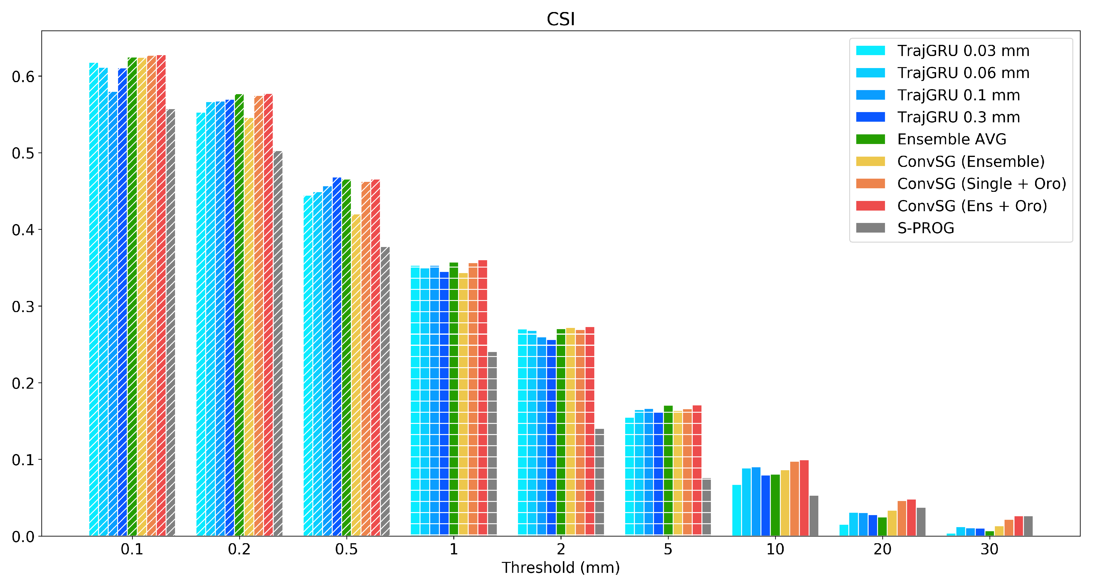
The overall evaluation results are summarized in

Table 2. CSI forecast skill of the ESG models compared with the ensemble (higher is better). In bold is the best result, the second best is underlined.

CSI Threshold (mm/h)	0.1	0.2	0.5	1	2	5	10	20	30
S-PROG	0.557	0.502	0.377	0.241	0.140	0.076	0.053	0.037	0.027
TrajGRU 0.03 mm	0.618	0.553	0.444	0.353	0.270	0.155	0.067	0.016	0.004
TrajGRU 0.06 mm	0.611	0.567	0.449	0.350	0.268	0.165	0.089	0.031	0.012
TrajGRU 0.1 mm	0.580	0.567	0.457	0.353	0.259	0.166	0.090	0.031	0.011
TrajGRU 0.3 mm	0.611	0.570	0.468	0.345	0.256	0.162	0.080	0.028	0.010
Ensemble AVG	0.625	0.577	0.466	0.357	0.270	0.171	0.081	0.025	0.007
ConvSG (Ensemble)	0.624	0.546	0.420	0.344	0.272	0.164	0.086	0.034	0.014
ConvSG (Single + Oro)	0.627	0.575	0.463	0.357	0.269	0.166	0.098	0.046	0.022
ConvSG (Ens + Oro)	0.628	0.577	0.466	0.360	0.273	0.171	0.099	0.048	0.026

and Figure 10, which report the comparison of the CSI (threat score) on the test set for three combinations of ConvSG, along with ensemble members, the mean, and S-PROG. Three combinations of ConvSG are shown: (i) the standard Stacked Generalization approach composed by all four members of the ensemble ConvSG (Ensemble); (ii) the orographic enhanced stacked generalization ConvSG (Ens + Oro); and (iii) the best of the four combination of each single model plus the orography ConvSG (Single + Oro). In this configuration, the best performance are achieved by the TrajGRU 0.03 mm model combined with orography.

Except for the threshold 0.5 mm, the full ESG model always outperforms all other deep learning combinations. The margin grows larger at the increase of the score threshold, and for very heavy rain rates (20 and 30 mm) all ESG model combinations register noticeable improvements over all members of the ensemble. At 30 mm, the full ESG model records a skill that is more than doubled with respect to the best performing ensemble member, and it is on par with the score reported by S-PROG, while retaining superior skills on all the other thresholds.

The second best performing model is ConvSG (Single + Oro), confirming that the addition of the orographic features induces substantial improvements on all rain regimes and particularly on the extremes. This is also reflected in the performance of the ConvSG (Ensemble) model, where a skill increase on the high rain rates, thus a reduction in CB, is paid with an inferior performance at lower rain rates.

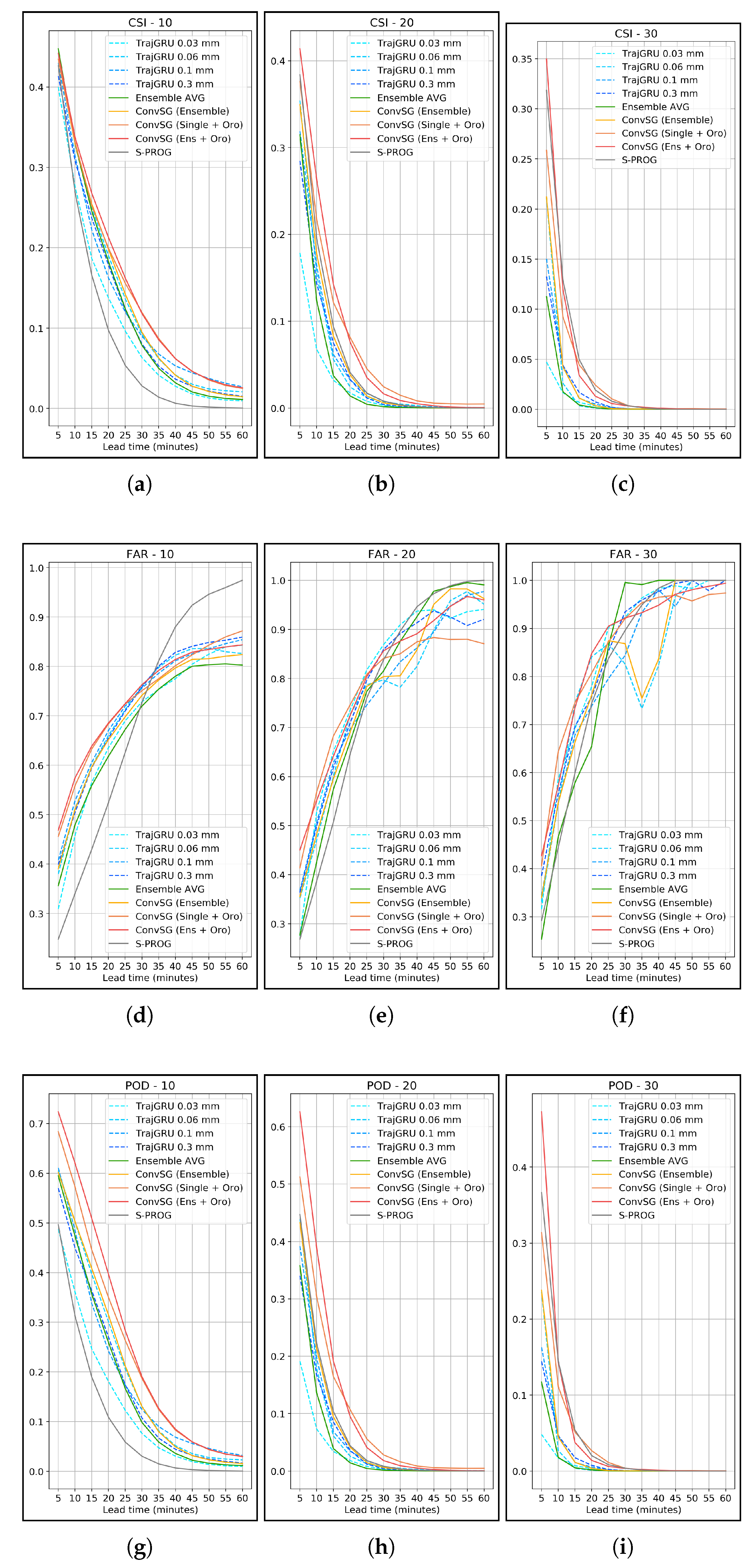
The framewise comparison shown in Figure 11 confirms that the increase in skill learned by all the ESG combinations is systematic and does not depend on temporal dimension: as such, the performance increases are consistent across all the predicted timesteps.

3.2. Continuous Scores

For the continuous scores, along with the standard Mean Squared Error (MSE) and Mean Absolute Error (MAE), we consider two scores that highlight the ability to forecast extreme events. One is the Conditional Bias itself (beta2) and the other is the Normalized Mean Squared Error (NMSE), a measure where differences on peaks have a higher weight than differences on other values.

The NMSE is expressed as:

$$\mathrm{NMSE}=\frac{{(P-O)}^2}{{(P+O)}^2}$$

(4)

where P is the prediction and O is the observation, while the CB is computed as the linear regression slope. All scores are reported in Figure 12. As expected, the stacked models substantially improve beta2 (Figure 12d) and NMSE (Figure 12b), but have a higher MSE (Figure 12a). S-PROG has a comparable CB with the full ESG model in the first lead times, but it is substantially outperformed by all the DL models on all the other measures.

Figure 13 shows an example output of the ConvSG (Ens + Oro) model on the test set, along with all members of the ensemble and the average. The ESG model handles better the overall variability, with less smoothing on the extremes.

4. Discussion

4.1. ConvSG Behavior

The results reported in Section 3 show that ConvSG can substantially improve the predictive skill of deep learning models on extreme rain rates. When the SG is trained only on the ensemble predictions, with no additional information, the ConvSG model is able to leverage the ensemble spread to trade off predictive performance on the lower rain rates for an improvement in high and extreme thresholds. This behavior is an instance of the no free lunch duality between the choice of reducing either CB or MSE. The study confirms that the balance between MSE minimization and CB is present also in deep learning models. On the other hand, the integration of orographic features extracted from the digital terrain model results in a gain in predictive skills over all the rain rates, with the largest improvements registered again on the high rain regimes. As expected, the best performing model is thus given by the combination of both the ensemble and the orography, where the skill score on the extremes is on par with S-PROG, whose skill is mainly driven by persistence.

4.2. Comparing ConvSG and S-PROG

While the score of S-PROG and ConvSG are similar on the extremes, there is also a fundamental qualitative difference between the predictions generated by the DL approach and the Lagrangian extrapolation. Indeed, the DL is able to to correctly model the growth and decay of the precipitation patterns in different locations in space. An example can be observed in Figure 13, where the ConvSG model is able to forecast the intensification of the rain rate in the upper section of the precipitation front, whereas S-PROG models a gradual decay. This ability opens the possibility for the DL model to eventually forecast new extremes, a behavior not possible by assuming Lagrangian persistence. This reflects in the trend reported by the CB score shown in Figure 12d: S-PROG has the best score in the first few frames but quickly decays to the worst score after 40 min of lead time. For the NMSE score (Figure 12b), S-PROG is competitive only in the first lead time, and quickly decays thereafter. Finally, for MSE and MAE (Figure 12a–c), ConvSG is superior to S-PROG because the two scores are more indicative of the skills obtained in the lower rain rates. This yields that an effective model evaluation and comparison can be correctly performed only when multiple thresholds for the categorical scores and multiple continuous scores are included in the analysis.

5. Conclusions and Future Work

We present a novel approach, leveraging a deep learning ensemble and stacked generalization, aimed at improving the forecasting skills of deep learning nowcasting models on extreme rain rates, thus reducing the conditional bias. The proposed method doubles the forecasting skill of a deep learning model on extreme precipitations, when combining the ensemble along with orographic features. Our contribution is threefold:

• the thresholded rainfall ensemble (TRE), where the same DL model and dataset can be used to train an ensemble of DL models by filtering precipitation at different rain thresholds;
• the Convolutional Stacked Generalization model (ConvSG) for nowcasting based on convolutional neural networks, trained to combine the ensemble outputs and reduce CB in the prediction; and
• the enhanced stacked generalization (ESG), where the SG approach is integrated with orographic features, to further improve prediction accuracy on all rain regimes.

The approach can close the skill gap between DL and traditional persistence-based methods on extreme rain rates, while retaining and improving the superior skill of the DL methods on lower rainfall thresholds, thus reaching equal or superior performance to all the analyzed methods on all the rainfall thresholds. As a drawback, its implementation requires a non-trivial amount of data and computation to train and correctly validate all model stack, along with some knowledge of the data distribution for the selection of the thresholds. Indeed, the presented ensemble size of four models was chosen as the minimum working example for TRE, to satisfy the computational budget limits for the deep learning stack. We thus expect that, incrementing the number of members and the corresponding thresholds, the contribution of the ensemble to the overall skill of the Stacked Generalization will increase. Further experiments are needed to more formally determine the thresholds and the number of the ensemble members required to maximize the desired skill improvements on the extremes. Moreover, despite the presented improvements, the absolute skill provided by nowcasting systems on extreme rainfall is still lagging in the single digit percentage, leaving the problem of extreme event prediction wide open for improvements. As future work, we plan to test the integration of new environmental variables in the ESG model along with orography, and to leverage the ensemble spread to generate probabilistic predictions.