Fire Behavior, Fuel Consumption, and Turbulence and Energy Exchange during Prescribed Fires in Pitch Pine Forests

Abstract

Prescribed fires are conducted extensively in pine-dominated forests throughout the Eastern USA to reduce the risk of wildfires and maintain fire-adapted ecosystems. We asked how fire behavior and fuel consumption during prescribed fires are associated with turbulence and energy fluxes, which affect the dispersion of smoke and transport of firebrands, potentially impacting local communities and transportation corridors. We estimated fuel consumption and measured above-canopy turbulence and energy fluxes using eddy covariance during eight prescribed fires ranging in behavior from low-intensity backing fires to high-intensity head fires in pine-dominated forests of the New Jersey Pinelands, USA. Consumption was greatest for fine litter, intermediate for understory vegetation, and least for 1 + 10 hour wood, and was significantly correlated with pre-burn loading for all fuel types. Crown torching and canopy fuel consumption occurred only during high-intensity fires. Above-canopy air temperature, vertical wind velocity, and turbulent kinetic energy (TKE) in buoyant plumes above fires were enhanced up to 20.0, 3.9 and 4.1 times, respectively, compared to values measured simultaneously on control towers in unburned areas. When all prescribed fires were considered together, differences between above-canopy measurements in burn and control areas (Δ values) for maximum Δ air temperatures were significantly correlated with maximum Δ vertical wind velocities at all (10 Hz to 1 minute) integration times, and with Δ TKE. Maximum 10 minute averaged sensible heat fluxes measured above canopy were lower during low-intensity backing fires than for high-intensity head fires, averaging 1.8 MJ m⁻² vs. 10.6 MJ m⁻², respectively. Summed Δ sensible heat values averaged 70 ± 17%, and 112 ± 42% of convective heat flux estimated from fuel consumption for low-intensity and high-intensity fires, respectively. Surprisingly, there were only weak relationships between the consumption of surface and understory fuels and Δ air temperature, Δ wind velocities, or Δ TKE values in buoyant plumes. Overall, low-intensity fires were effective at reducing fuels on the forest floor, but less effective at consuming understory vegetation and ladder fuels, while high-intensity head fires resulted in greater consumption of ladder and canopy fuels but were also associated with large increases in turbulence and heat flux above the canopy. Our research quantifies some of the tradeoffs involved between fire behavior and turbulent transfer of smoke and firebrands during effective fuel reduction treatments and can assist wildland fire managers when planning and conducting prescribed fires.

1. Introduction

Prescribed fires are conducted extensively throughout North America because they are one of the most cost-effective methods to reduce hazardous fuels and mitigate the risk of severe wildfires [1,2,3,4]. In the Eastern USA, prescribed fires are also essential for the maintenance of fire-adapted ecosystems, such as those dominated by pines and oaks [5,6,7,8]. Beneficial aspects of fire in promoting biodiversity in pine- and oak-dominated forests are well documented [6,9,10,11]. In addition, prescribed fires may enhance forest resilience to other disturbances such as insect infestations [12,13]. However, because prescribed fires can result in significant emissions of particulate matter and regulated pollutants, smoke management has become an important issue when they are conducted near larger human population centers in the Eastern USA [14,15,16]. Additional constraints to the use of prescribed fire involve reducing the risk of escapes by limiting ember production and transport and controlling fire perimeters in areas with high property values.

Fire behavior during prescribed fires is influenced by a number of factors, including fuel loading and arrangement [1,17,18,19], fuel moisture content, previous and current weather conditions [20], and ignition pattern [21]. Fuel loading and consumption during prescribed fires have been quantified throughout fire-adapted forest ecosystems in the Eastern USA, and several studies have documented significant linear relationships between initial fuel loading and consumption of forest floor and understory vegetation across a range of fire intensities [19,22,23]. Wildland fire managers typically conduct prescribed burns within a constrained range of fuel moisture contents and meteorological conditions, with wind speed, ambient air temperature and relative humidity especially important for maintaining desired fire behavior and fire line control. Ignition pattern influences fire behavior because commonly employed spot or linear ignitions can result in a variety of fire behaviors, ranging from low-intensity backing fires to high-intensity head fires with crowning behavior.

Quantitative information on how firing pattern and the resultant fire behavior control the consumption of surface, understory and canopy fuels during prescribed fires is important for optimizing the effectiveness of fuel reduction treatments, while simultaneously minimizing the adverse impacts of smoke dispersion on local air quality and firebrand transport on unwanted ignitions. Low-intensity backing fires reduce surface and understory fuels, but when conducted under conditions where smoke dispersion is inadequate, they can result in undesirable impacts of smoke in local communities and along transportation corridors. In contrast, high-intensity fires can achieve fuel reduction objectives and adequate smoke dispersion, but ember transport and increased difficulty in fire line control enhances the risk of escapes. Despite the benefits and increased use of prescribed fire, tradeoffs between fire behavior, consumption of fuels, and turbulence and energy fluxes in buoyant plumes which control smoke dispersion and ember transport remain to be evaluated for many fire-adapted forests in the Eastern USA [15,24,25].

Our central objective was to quantify how fire behavior and fuel consumption were related to turbulence and energy fluxes across a range of fire intensities. More specifically, we asked what the relationships between fuel loading and consumption are during low- and high-intensity prescribed fires conducted by State and Federal wildland fire managers in the Pinelands National Reserve (PNR) of Southern New Jersey, and how in turn does fire intensity influence above-canopy turbulent transfer and heat fluxes in the fire environment. 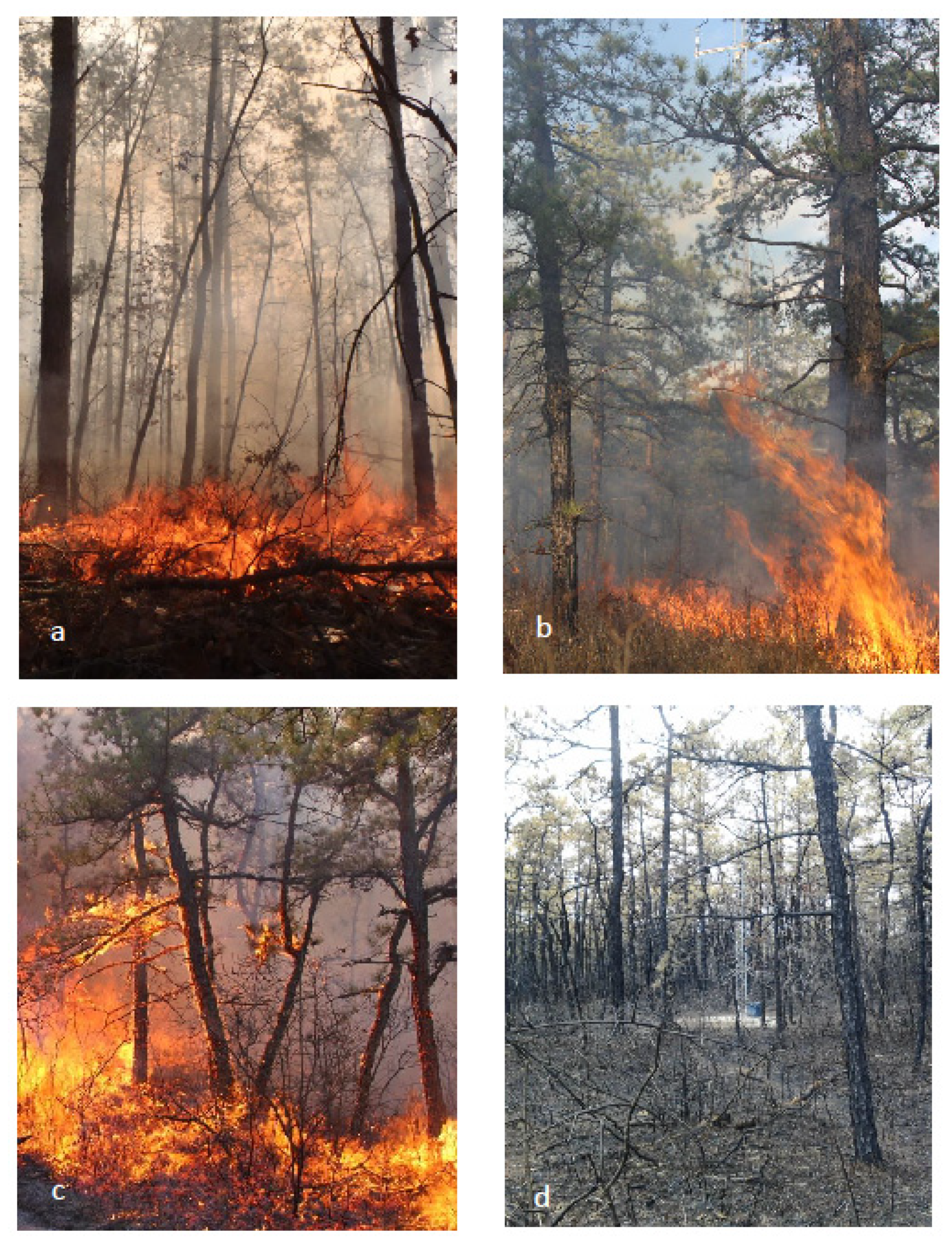We concentrated our efforts on sites dominated by pitch pine (Pinus rigida Mill.) and shortleaf pine (Pinus echinata Mill.), because these have a higher incidence of wildfires compared to other forest types in the Northeast USA and are a major focus of fuel reduction treatments by State and Federal wildland fire managers in the PNR [26,27,28,29]. They are also adjacent to densely populated suburban areas and transportation networks where smoke management and fire line control are critical. We analyzed new and previously published data from eight prescribed fires, ranging in intensity from low-intensity backing fires to high-intensity head fires. Five low-intensity fires resulted from either the ignition of backing fires or relatively low initial surface and understory fuel loads, and three high-intensity fires resulted from either a flanking fire with some crown torching or the ignition of head fires. We then evaluated the relationships between predominant fire behavior and fire intensity, loading and consumption of surface, understory and canopy fuels, and above-canopy turbulence and energy fluxes.

2. Materials and Methods

2.1. Site Description

Research sites were located in Burlington and Ocean Counties in the Pinelands National Reserve (PNR). The PNR is the largest continuous forested landscape on the Northeastern coastal plain and is characterized by a higher frequency and intensity of wildfires compared to other forest ecosystems in the Northeastern USA [27,30,31]. In the last decade, the area burned in prescribed fires in the PNR has exceeded that burned in wildfires by twofold [29]. The climate is cool temperate, with mean monthly temperatures of 0.3 and 23.8 °C in January and July, respectively (1986–2016; [32]). Mean annual precipitation is 1123 ± 182 mm (mean ± 1 SD). Soils are derived from the Cohansey and Kirkwood Formations, and are sandy, coarse-grained, and have low nutrient status.

To quantify the relationships between fire intensity, fuel consumption, and turbulence and heat flux, we selected six pine-dominated forest sites for intensive study. Two of the sites were burned twice during the 10 year study period for a total of eight prescribed fires (

Table 1. Forest type and experimental design for the eight prescribed fires conducted in the New Jersey Pinelands National Reserve. Data are forest type, site location and date of the burn, number of towers within each burn area, number of control towers, and predominant fire behavior when flame fronts reached the tower(s).

Forest Type	Site	Date	Burn Area Towers	Control Towers	Predominant Fire Behavior
Low-intensity fires
Pine–oak	Fort Dix 1	02/09/2006	1	2	Backing fire
Pine–scrub oak	Cedar Bridge 1	03/22/2008	1	2	Backing fire
Pine–oak	Silas Little 2	03/06/2012	1	2	Backing fire
Pine–scrub oak	Cedar Bridge 1	03/15/2013	1	2	Backing fire
Pine–scrub oak	Warren Grove	03/09/2015	3	1	Mixed
High-intensity fires
Pine–oak	Butler Place 2	03/20/2011	1	2	Flanking fire
Pine–scrub oak	Warren Grove 3	03/05/2013	3	1	Head fire
Pine–scrub oak	Warren Grove 3	03/11/2014	3	1	Head fire

¹ Fuel loading and consumption previously published in [23]. ² Turbulence statistics previously published in [15,25]. ³ Fuel loading and consumption, and detailed fire behavior previously published in [36].

). Three sites were pine–scrub oak stands, dominated by pitch pine (Pinus rigida Mill.), with scattered overstory blackjack and white oaks (Quercus stellata Wangenh., Q. alba L,) and abundant scrub oaks (Q. marlandica Muenchh., Q. ilicifolia Wangenh.) in the understory, and three were pine–oak stands, with pitch pine, shortleaf pine (P. echinata Mill.), chestnut oak (Q. prinus L.), white oak, black oak (Q. velutina Lam.), and scarlet oak (Q. coccinea Muenchh.) in the overstory and scrub oaks in the understory (Table 1). All sites had moderate to dense shrub cover in the understory, primarily blueberry (Vaccinium spp.), huckleberry (Gaylussacia spp.), and laurels (Kalmia spp.), and sedges, mosses and lichens also were present. Despite the prevalence of sandy, well-drained, nutrient-poor soils, stands are moderately productive, and fuels on the forest floor and in the understory can accumulate rapidly [23,33,34].

2.2. Prescribed Fires

Prescribed fires were conducted by Federal wildland fire managers (pine–oak site at Fort Dix in 2006) or the New Jersey Forest Fire Service personnel (all other sites) during the typical prescribed burn window between early February and late March (New Jersey Forest Fire Service, pers. com). All burns were conducted within the prescription window for prescribed fires in the PNR, with cool air temperatures, relative humidity between 20% and 39%, and low to moderate mean ambient wind velocities (

Table 2. Meteorological conditions during the eight prescribed burns conducted in the New Jersey Pinelands National Reserve. Data are forest type, site location, date of the prescribed fire, and mean ambient air temperature, relative humidity and wind velocity measured above canopy (12.5 to 19.5 m height) from 12:00 to 16:00 LT (mean ± 1 SD).

Forest Type	Site	Date	Air Temp (°C)	RH (%)	Wind (m s−1)
Low-intensity fires
Pine–oak	Fort Dix	02/09/2006	0.9 ± 0.9	31.1 ± 3.0	3.0 ± 0.3
Pine–scrub oak	Cedar Bridge	03/22/2008	9.0 ± 1.3	34.9 ± 7.1	2.2 ± 0.4
Pine–oak	Silas Little	03/06/2012	5.8 ± 1.4	21.6 ± 2.2	2.2 ± 0.3
Pine–scrub oak	Cedar Bridge	03/15/2013	7.2 ± 1.2	34.3 ± 2.0	4.3 ± 0.6
Pine–scrub oak	Warren Grove	03/09/2015	3.7 ± 0.9	20.2 ± 1.1	2.7 ± 0.4
High-intensity fires
Pine–oak	Butler Place	03/20/2011	8.6 ± 1.9	37.1 ± 8.4	2.1 ± 0.6
Pine–scrub oak	Warren Grove	03/05/2013	7.6 ± 1.0	38.6 ± 3.6	1.5 ± 0.3
Pine–scrub oak	Warren Grove	03/11/2014	16.7 ± 1.1	33.1 ± 4.5	2.9 ± 0.4

). Initial surface and understory fuel loads were low to intermediate, based on previously published estimates across the PNR [23,29,35]. Fires were ignited using drip torches, and an appropriate ignition pattern was employed to create the predominant fire behavior during each prescribed fire (Figure 1). Linear ignitions were used to produce low-intensity, predominantly backing fires during four of the burns (two were conducted five years apart in the same pitch pine–scrub oak stand). In the fifth stand, a head fire was initially ignited, but relatively low surface and understory fuel loads resulted in a low-intensity fire across the majority of the burn area. The remaining three high-intensity fires resulted from a flanking fire with some crown torching in one of the stands, and two head fires with significant crown torching that were ignited using linear ignitions in the other two stands. Experimental conditions including stand composition, predominant fire behavior, and meteorological conditions are summarized in Table 1 and Table 2. Further details of each fire appear in [15,23,25,36].

2.3. Fuel Loading and Consumption Estimates

Initial and post-burn fuel loading for each prescribed fire were estimated by destructively harvesting understory vegetation and the forest floor in 1.0 m² plots (n = 10 to 36 for each burn) located randomly within 150 m of the flux towers described below. Shrubs, scrub oaks, seedlings and saplings <2.0 m tall were clipped to the level of the forest floor, sorted into foliage and 1 hour (<0.64 cm diameter) and 10 hour (>0.64 cm and <2.54 cm diameter) stems, dried at 70 °C and weighed when dry. Fine litter, consisting of primarily needles, leaves, and miscellaneous material, and 1 hour and 10 hour wood in the litter layer (L horizon) of the forest floor were collected in the same 1.0 m² plots, sieved through 2 mm mesh when necessary to remove undifferentiated organic matter and sand, sorted and then dried at 70 °C and weighed. Moisture content of available fuels during each prescribed fire was estimated from samples of pitch pine needles, 1 hour pitch pine stems, 1 hour shrub stems, and fine litter and 1 hour and 10 hour woody fuels on the forest floor at intervals throughout each burn (deciduous oaks and understory shrubs were leafless at the time of the burns). Samples were placed in sealed plastic bags and stored in coolers (<24 hours), and then weighed before and after drying at 70 °C until dry to estimate moisture content. Following each burn, 1.0 m² plots located near the pre-burn plots were sampled and sorted in an identical manner, and then dried at 70 °C and weighed when dry. Available fuels in pitch pine canopies were estimated for the three high-intensity fires using pre- and post-burn Light detection and ranging (LiDAR) acquisitions calibrated to estimate canopy bulk density (kg m⁻³) in 1 m layers [36,37,38].

2.4. Eddy Covariance and Meteorological Measurements

To monitor turbulence and energy fluxes in the fire environment, we installed above-canopy towers with eddy covariance instrumentation in each stand to be burned. Towers in burn areas were paired with above-canopy towers in unburned stands within a 100 m to 15 km radius to serve as controls (Table 1). Three-dimensional turbulence and air temperature were measured at the top of each tower using sonic anemometers (RM 80001V, R. M. Young, Inc., Traverse City, MI, USA or Windmaster Pro, Gill Instruments Ltd., Lymington, UK). Sonic anemometers were mounted 2 to 4 m above the canopy in each stand (13 to 20 m above the ground). Sonic anemometer data were recorded at 10 Hz using Campbell Scientific CR 3000 data loggers (Campbell Scientific, Inc., Logan, UT, USA) or laptop computers. In addition to sonic anemometers, prescribed burns conducted from 2011 to 2015 employed thermocouples (Omega SSRTC-GG-K-36, Omega Engineering, Inc., Stamford, CT, USA) mounted at intervals along each tower (1 m height intervals up to 10 m, and then every 2.5 m interval to 20 m height for burns conducted in 2011 and 2012, and at 1.5 m intervals to the top of each tower in 2013–2015). All thermocouples were logged at 10 Hz using CR-3000 data loggers (Campbell Scientific, Inc., Logan, UT, USA).

At the control towers, identical turbulence and thermocouple measurements were made, along with additional meteorological measurements made on the above-canopy towers and on 3 m tall understory towers located nearby. Incoming shortwave radiation (LI-200, LI-COR, Inc., Lincoln, NE, USA), net radiation (NRLite, Kipp and Zonen, Inc., Delft, The Netherlands), air temperature and relative humidity (HMP45 or HMP50, Vaisala, Inc., Woburn, MA, USA), wind speed and direction (05013-5, R. M. Young Co., Traverse City, MI, USA), and precipitation (TE525, Texas Electronics, Inc., Dallas, TX, USA) were measured at ca. 12–19 m height on the above-canopy towers, and at 2 m height on the understory towers. Soil heat flux was measured using one to three heat flux transducers (#HFT-3.1, Radiation and Energy Balance Systems, Inc., Seattle, WA, USA) buried at 10 cm depth within 10 m of each control tower, and soil temperature was measured at 5 cm depth (CS-107 or CS-109, Campbell Scientific, Inc.). All meteorological data were recorded with data loggers (CR10x, CR23x and CR1000, Campbell Scientific, Inc.).

During three of the low-intensity fires (the pine–oak stand at Fort Dix in 2006 and the pitch pine–scrub oak stand at Cedar Bridge in 2008 and 2013), water vapor concentrations were measured above canopy using a LI-COR LI-7000 carbon dioxide and water vapor analyzer (LI-COR Inc., Lincoln, NE, USA) operating at 10 Hz and logged with a laptop computer to estimate latent heat fluxes. Identical water vapor measurements were made simultaneously on above-canopy control towers [39].

2.5. Data and Statistical Analyses

Consumption of fine litter, woody fuels and understory vegetation was estimated by subtracting post- from pre-burn dry weights for each fuel type. Pearson’s product moment correlation coefficients were calculated for the relationship between pre-burn loading and estimated consumption of each fuel type using Sigmaplot (Version 12.5, SYSTAT Software, Inc., San Jose, CA, USA). Heat release per unit area was calculated from consumption estimates of each fuel type using 18.7 KJ g⁻¹ as the heat of combustion (Appendix A). Energy consumed during preheating and pyrolysis of fuels was calculated as a function of the dry mass, moisture content, and initial ambient temperature of each fuel type consumed using Equation (A1) in Appendix A. Following [40], we assumed that radiant heat flux accounted for approximately 17% of total heat of combustion of each fuel type, and radiant heat flux was calculated using Equation (A2) in Appendix A. Latent heat flux from combusted fuels was calculated using the dry mass and moisture content of each fuel type, assuming complete vaporization of the moisture in consumed fuels using Equation (A3) in Appendix A. The remaining heat flux was assumed to be convective heat, energy consumed in forest floor and soil heating, and heat storage in the canopy airspace [39,40].

Pearson’s product moment correlation coefficients were calculated for the relationship between sonic air temperature and vertical and horizontal wind velocities measured at 10 Hz for periods when air temperatures exceeded 5 °C above ambient, which typically occurred when flame fronts were beneath or within close proximity of towers during the prescribed fires. Sonic air temperature and vertical and horizontal wind velocities were then integrated from 10 Hz raw data to 1 second and 1 minute intervals. Maximum differences in air temperature or vertical and horizontal wind velocities between burn area and control towers for 10 Hz and 1 second and 1 minute integration times were designated as Δ values, and occurred at the time of flame front passage or when fires were in closest proximity to towers in burn areas. Correlation coefficients were calculated for the relationships between Δ air temperature and Δ vertical or horizontal wind velocities at the appropriate intervals. Correlation coefficients were also calculated for relationships between consumption of fuel types and Δ air temperature or Δ wind velocity statistics. Turbulent kinetic energy (TKE; m⁻² s⁻²) was calculated at 1 minute intervals for all sonic anemometer data collected at burn area and control towers using Equation (A4) in Appendix A. Correlation coefficients were then calculated for the relationships between TKE values and Δ air temperature, and between TKE values and fuel consumption estimates.

Friction velocity (u*, m s⁻¹) and sensible heat fluxes (H, W m⁻²) were calculated from coordinate-rotated wind velocities and sonic temperature data using instantaneous (10 Hz) deviations from 10 minute block averages using EdiRe software (Equations (A5) and (A6) in Appendix A; [41]). Maximum differences of u* and sensible heat flux between burn area and control towers were then calculated for each 10 minute period. At the low-intensity burns conducted at the pine–oak stand at Fort Dix in 2006 and the pitch pine–scrub oak stand at Cedar Bridge in 2008 and 2013, latent heat fluxes were calculated for 10 minute periods using EdiRe software (Equation (A7) in Appendix A; see [39] for details on measurements of latent heat fluxes and energy balance at these stands). Differences in sensible and latent heat fluxes (in MJ m⁻²) between burn area and control towers were then integrated over the period of each burn and compared to estimates calculated for the sum of consumed fuels.

3. Results

3.1. Fuel Loading and Consumption

Pre-burn forest floor and understory fuel loading differed by a factor of 2.2 among stands, and was least at the pine–scrub oak stand at Warren Grove burned in 2015 that had been burned two years previously during an intense head fire, and greatest at the pine–scrub oak stand at Cedar Bridge burned in 2008 that had burned 13 years previously in a wildfire (Figure 2,

Table A1. Understory and forest floor fuel loading measured pre- and post-burn, fuel moisture content sampled during each burn, estimated consumption, percent estimated consumption, and the contribution of individual types to total fuel consumption for eight prescribed fires conducted in the Pinelands National Reserve. Presentation order follows initial total surface and understory fuel loading from lowest to highest within category of burn intensity. Values are the means ± 1 SD, and “nm” is not measured.

Forest Type/Site	Pre-Burn	Fuel Moisture	Post-Burn	Consumption
	(g m−2)	(%)	(g m−2)	(g m−2 and %; % of Total)
Low-intensity fires
Pine–scrub oak (Warren Grove 2015; n = 36)
Understory	230 ± 122	54 ± 4	95 ± 51	134	58%	29%
Fine litter	558 ± 152	28 ± 14	224 ± 71	334	60%	71%
1 hour wood	100 ± 67	nm	88 ± 32	12	12%	3%
10 hour wood	77 ± 49	nm	89 ± 55	−11	-14%	-2%
Total	965 ± 235		495 ± 161	469	49%
Pine–oak (Silas Little Exp. For. 2012; n = 24)
Understory	170 ± 132	53 ± 6	127 ± 56	43	25%	8%
Fine litter	747 ± 116	43 ± 13	311 ± 78	436	58%	86%
1 hour wood	113 ± 67	nm	95 ± 42	18	16%	4%
10 hour wood	74 ± 73	56 ± 6	64 ± 65	10	14%	2%
Total	1104 ± 246		597 ± 134	507	46%
Pine–scrub oak (Cedar Bridge 2013; n = 10)
Understory	411 ± 334	59 ± 7	176 ± 93	235	57%	24%
Fine litter	785 ± 259	48 ± 12	204 ± 68	581	74%	59%
1 hour wood	182 ± 134	48 ± 18	59 ± 25	123	68%	12%
10 hour wood	187 ± 142	51 ± 17	138 ± 122	49	26%	5%
Total	1565 ± 583		577 ± 114	988	63%
Pine–oak (Fort Dix 2006; n = 15)
Understory	486 ± 360	52 ± 8	199 ± 155	287	59%	36%
Fine litter	933 ± 360	27 ± 6	423 ± 164	510	55%	63%
1 + 10 hour wood	191 ± 125	nm	185 ± 98	6	3%	1%
Total	1610 ± 520		807 ± 293	803	50%
Pine–scrub oak (Cedar Bridge 2008; n = 10)
Understory	445 ± 102	50 ± 7	301 ± 133	144	32%	14%
Fine litter	1492 ± 359	44 ± 11	712 ± 178	780	52%	78%
1 + 10 hour wood	207 ± 97	16 ± 5	129 ± 44	78	38%	8%
Total	2144 ± 350		1142 ± 225	1002	47%
High-intensity fires
Pine–oak (Butler Place 2011; n = 27)
Understory	632 ± 289	53 ± 8	268 ± 175	364	58%	53%
Fine litter	732 ± 232	23 ± 11	446 ± 150	287	39%	41%
1 hour wood	73 ± 56	21 ± 8	34 ± 36	39	53%	6%
10 hour wood	41 ± 63	27 ± 5	41 ± 66	0	0%	0%
Total	1478 ± 388		789 ± 269	689	47%
Pine–scrub oak (Warren Grove 2013; n = 36)
Understory	380 ± 219	59 ± 10	114 ± 86	266	70%	26%
Fine litter	741 ± 80	19 ± 10	217 ± 56	524	71%	50%
1 hour wood	294 ± 174	25 ± 22	107 ± 25	186	63%	18%
10 hour wood	133 ± 122	32 ± 18	66 ± 26	67	50%	6%
Total	1547 ± 327		504 ± 136	1042	67%
Pine–scrub oak (Warren Grove 2014; n = 36)
Understory	473 ± 134	52 ± 8	123 ± 79	350	74%	30%
Fine litter	963 ± 232	46 ± 14	272 ± 69	691	72%	60%
1 hour wood	163 ± 88	46 ± 14	83 ± 27	80	49%	7%
10 hour wood	103 ± 80	nm	66 ± 60	37	36%	3%
Total	1702 ± 307		543 ± 131	1158	68%

). Initial loading of fine litter, 1 hour woody, and 10 hour woody fuels on the forest floor and in the understory was similar among stands burned at the different fire intensities, averaging 1478 ± 467 g m⁻² and 1576 ± 115 g m⁻² (mean ± 1 SD) for the low-intensity and high-intensity burns, respectively. Fine litter on the forest floor was the dominant fuel type, with the proportion of fine litter representing 61 ± 8% of total surface and understory fuels in the five stands burned in low-intensity fires, and 51 ± 5% in the three stands burned in high-intensity fires (Figure 2, Table A1).

Consumption of surface fuels and understory vegetation during prescribed burns differed by a factor of 2.5 among stands, while percent consumption ranged from 46% to 68% of total pre-burn loading (Figure 2, Table A1). Consumption of fine litter on the forest floor was greatest and consumption of 1 hour and 10 hour woody fuels on the forest floor the least during all fires except during the high-intensity fire conducted in a pine–oak stand in 2011, where estimated consumption of understory vegetation exceeded fine fuel consumption (Table A1). Consumption of surface and understory fuels was significantly related to pre-burn loading, accounting for 58%, 85%, 75%, and 60% of the variability for fine litter, woody fuels, understory vegetation and total fuel consumption, respectively (Figure 3,

Table 3. Linear models of pre-burn loading and consumption of understory vegetation, fine litter on the forest floor, woody fuels on the forest floor, and total surface and understory fuels during the eight prescribed fires. Data are shown in Figure 3 and were fit to the equation, consumption = α × initial mass + β; the units are g m⁻².

Fuel Type	α ± 1 SE	β ± 1 SE	r2	F1,8	P
Understory stems 1	0.644 ± 0.137	−31.9 ± 57.6	0.751	22.1	<0.01
fine litter	0.536 ± 0.164	62.6 ± 152.0	0.582	10.7	<0.02
1 + 10 hour wood	0.787 ± 0.122	−103.8 ± 32.0	0.853	41.5	<0.001
Total	0.622 ± 0.184	−98.8 ± 291.8	0.598	11.4	<0.02

¹ Includes live and dead stems of shrubs and scrub oaks <2 m tall in 1 + 10 hour size classes.

). There was little relationship between burn intensity and the proportion of fine or woody fuels consumed on the forest floor (see below), but there was a trend towards greater proportional consumption of understory vegetation in the more intense fires; consumption represented 39%, 50 ± 15%, and 67 ± 9% of initial understory loading for the two low-intensity fires with the lowest surface and understory fuel loading, the three low-intensity fires with greater surface and understory fuel loading, and the three high-intensity fires, respectively. In contrast to surface and understory fuel consumption, canopy fuel consumption was minimal during all low–intensity prescribed burns, while it represented up to 21% of estimated available fuels in the high–intensity head fires (Table A1; see also [36]).

Estimated heat release from the combustion of surface, understory and canopy fuels averaged 15.0 ± 6.0 and 21.3 ± 6.6 MJ m⁻² for the low- and high-intensity fires, respectively (Figure 4a). When the low-intensity fires were separated by relatively low and moderate initial surface and understory fuel loading, estimated heat release was 9.2 and 18.9 ± 3.9 MJ m⁻², respectively. Estimated latent and convective heat fluxes together averaged 78% of the total heat of combustion for all fires (Figure 4a).

3.2. Turbulence and Energy Exchange During Prescribed Fires

Maximum values for air temperature and vertical wind velocity measured at 10 Hz averaged 5.7 and 1.1 times greater than control tower values for low-intensity burns, and 9.5 and 2.1 times greater than control tower values for high-intensity burns, respectively (

Table A2. Above-canopy air temperature, vertical wind velocities, and horizontal wind velocities measured at 10 Hz and then integrated over 1 second and 1 minute averaging times on towers located in burn area and control stands during the eight prescribed fires.

Site/Date	Air Temperature (°C)			Vertical Wind Velocity (m s−1)			Horizontal Wind Velocity (m s−1)			TKE
	10 Hz	1 sec	1 min	10 Hz	1 sec	1 min	10 Hz	1 sec	1 min	1 min
Low-intensity burns
Pine–oak 2006
Burn area	24.4	21.4	8.4	4.03	3.09	1.38	11.04	10.32	6.52	5.466
Control 1	2.5	2.3	1.6	3.65	2.74	0.64	10.04	9.16	6.23	4.039
Control 2	2.9	2.6	1.5	4.08	3.10	0.55	10.53	8.08	5.20	4.655
Δ Values	21.7	18.9	6.9	0.17	0.17	0.79	0.75	1.70	0.81	1.119
Pine–scrub oak 2008
Burn area	49.3	39.4	11.8	3.79	2.84	0.73	8.50	8.29	5.65	3.526
Control 1	11.2	11.0	9.7	3.63	2.84	0.71	8.99	8.02	4.67	3.807
Control 2	11.2	10.9	9.4	3.43	2.78	0.75	9.72	9.04	5.18	3.047
Δ Values	38.2	26.9	2.3	0.26	0.03	0.00	−0.86	−0.24	0.72	0.099
Pine–oak 2012
Burn area	31.8	24.6	12.1	3.28	2.27	0.69	8.16	7.39	5.33	3.172
Control 1	6.6	6.5	5.9	2.95	2.19	0.89	8.34	7.61	5.76	3.266
Control 2	9.4	9.2	8.2	3.76	2.45	0.77	9.24	8.08	5.33	3.364
Δ Values	23.8	16.7	5.1	−0.14	−0.05	−0.14	−0.63	−0.46	−0.22	−0.143
Pine–scrub oak 2013
Burn area	51.5	34.1	13.9	5.78	3.94	0.70	13.94	12.78	7.22	8.674
Control 1	11.2	10.8	10.2	5.16	3.22	0.72	14.90	13.85	9.83	8.837
Control 2	11.3	11.2	10.0	5.42	3.01	0.48	14.83	13.09	5.95	8.163
Δ Values	40.3	23.1	3.8	0.49	0.83	0.09	−0.93	−0.70	−0.67	0.174
Pine–scrub oak 2015
Burn area north	67.6	57.3	21.0	5.93	3.64	1.38	9.28	7.64	4.49	3.252
Burn area south	49.3	36.7	17.4	3.86	3.00	0.98	11.15	8.44	5.09	5.130
Burn area west	37.3	27.9	9.7	3.71	2.72	0.58	9.55	8.47	5.29	3.688
Control 1	8.2	8.0	6.6	3.20	2.60	0.53	9.28	8.10	5.23	3.636
Δ Values	43.2	32.6	9.5	1.30	0.52	0.45	0.71	0.08	−0.27	0.387
High-intensity burns
Pine–oak 2011
Burn area	121.0	100.64	49.0	8.26	5.25	2.62	12.73	9.64	6.18	7.700
Control 1	11.3	10.83	8.5	3.35	2.64	0.67	8.64	7.90	5.32	3.276
Control 2	11.4	11.00	9.9	4.03	3.25	0.99	9.12	8.59	5.98	3.277
Δ Values	109.6	89.73	39.9	4.57	2.31	1.79	3.86	1.39	0.53	4.424
Pine–scrub oak 2013
Burn area north	122.8	109.6	41.9	9.37	9.37	1.78	6.43	13.35	4.76	9.372
Burn area south	332.1	228.1	78.4	10.32	7.22	2.08	16.01	8.27	3.95	7.357
Burn area west	159.3	129.1	42.0	6.22	4.47	2.52	10.02	6.31	4.12	4.851
Control 1	10.3	9.9	8.8	2.20	1.50	0.40	12.84	5.90	3.84	1.746
Δ Values	194.5	145.7	45.3	6.44	5.52	1.38	6.41	2.20	0.44	5.447
Pine–scrub oak 2014
Burn area north	233.0	198.8	76.8	9.04	5.82	2.55	13.42	11.17	6.54	6.949
Burn area south	154.0	100.8	38.8	9.35	5.56	1.16	14.60	10.63	6.46	8.938
Burn area west	113.4	63.4	27.8	5.78	4.09	1.08	14.71	10.05	6.26	6.731
Control 1	20.9	20.4	19.0	4.34	3.19	0.43	11.40	10.31	5.90	5.034
Δ Values	145.9	100.6	28.8	3.72	1.97	1.17	2.84	0.31	0.52	2.505

). Relationships between air temperatures ≥5 °C above ambient and vertical wind velocities measured at 10 Hz in buoyant plumes were weaker for low-intensity fires than for high-intensity fires (Figure A1;

Table A3. Linear models of air temperature and vertical wind velocity measured at 10 Hz on burn area towers during the eight prescribed fires when air temperature was ≥5 °C above ambient air temperature measured on control towers shown in Figure A1. Values are air temperature at ≥5 °C above ambient air temperature, number of 10 Hz values ≥ 5 °C above ambient air temperature when flame fronts were in the vicinity of each tower, and slopes, intercepts and Pearson’s correlation coefficients for linear relationships. Data were fit to the equation y = α × (variable) + β.

Stand/Date	Air Temp (°C)	10 Hz values	α	β	r2
Low-intensity fires
Pine–oak 2006	7.0	3882	0.094 ± 0.006	0.232 ± 0.059	0.062
Pine–scrub oak 2008	15.0	1132	0.030 ± 0.004	0.762 ± 0.079	0.040
Pine–oak 2012	12.0	487	0.074 ± 0.009	−0.107 ± 0.070	0.108
Pine–scrub oak 2013 (Figure 5a)	15.0	2171	0.073 ± 0.004	−0.051 ± 0.079	0.134
Pine–scrub oak 2015
North (Figure 5b)	12.0	2743	0.042 ± 0.002	0.533 ± 0.034	0.203
South	12.0	1250	0.044 ± 0.003	0.520 ± 0.062	0.146
West	12.0	1980	0.062 ± 0.003	0.175 ± 0.055	0.160
High-intensity fires
Pine–oak 2011 (Figure 5c)	15.0	3268	0.047 ± 0.001	0.262 ± 0.041	0.371
Pine–scrub oak 2013
North	14.0	1413	0.039 ± 0.002	0.417 ± 0.074	0.266
South	14.0	2493	0.038 ± 0.001	−0.394 ± 0.040	0.305
West (Figure 5d)	14.0	1263	0.035 ± 0.001	0.142 ± 0.055	0.384
Pine–scrub oak 2014
North	24.0	861	0.028 ± 0.109	0.281± 0.109	0.281
South	24.0	1654	0.036 ± 0.002	−0.009 ± 0.072	0.201
West	24.0	2873	0.028 ± 0.002	0.393 ± 0.063	0.087

). The slopes of these relationships were generally lower for high-intensity burns, averaging 0.036 ± 0.007 (mean ± 1 SD) versus 0.060 ± 0.022 for high- and low-intensity burns, respectively. Increasing integration times from 10 Hz to 1 minute resulted in consistent decreases in peak air temperature and vertical wind velocities in burn areas relative to measurements on control towers (designated as Δ values), while differences in horizontal wind velocities were more variable during low-intensity fires (

Table 4. Maximum differences of above-canopy air temperature, vertical wind velocity, and horizontal wind velocity measured at 10 Hz and integrated over 1 second and 1 minute averaging times on towers located in burned areas and control stands during the eight prescribed fires.

Stand/Date	Δ Air Temperature (°C)			Δ Vertical Wind (m s−1)			Δ Horizontal Wind (m s−1)
	10 Hz	1 sec	1 min	10 Hz	1 sec	1 min	10 Hz	1 sec	1 min
Low-intensity fires
Pine–oak 2006	21.7	18.9	6.9	0.17	0.17	0.79	0.75	1.70	0.81
Pine–scrub oak 2008	38.2	26.9	2.3	0.26	0.03	0.00	−0.86	−0.24	0.72
Pine–oak 2012	23.8	16.7	5.1	−0.14	−0.05	−0.14	−0.63	−0.46	−0.22
Pine–scrub oak 2013	40.3	23.1	3.8	0.49	0.83	0.09	−0.93	−0.70	−0.67
Pine–scrub oak 2015	43.2	32.6	9.5	1.30	0.52	0.45	0.71	0.08	−0.27
High-intensity fires
Pine–oak 2011	109.6	89.7	39.5	4.75	2.31	1.79	3.86	1.39	0.53
Pine–scrub oak 2013	194.5	145.7	45.3	6.44	5.52	1.38	6.41	2.20	0.44
Pine–scrub oak 2014	145.9	100.6	28.8	3.72	1.97	1.17	2.84	0.31	0.52

). When all prescribed fires were considered together, relationships between maximum Δ air temperatures and Δ vertical wind velocities, between maximum Δ air temperatures and Δ horizontal wind velocities, and between maximum Δ vertical and Δ horizontal wind velocities measured at 10 Hz were highly significant (

Table 5. Linear models of maximum differences (Δ values) for air temperature, vertical wind velocity, and horizontal wind velocity measured at 10 Hz and integrated over 1 second and 1 minute averaging times on towers in burn areas and control stands during the eight prescribed fires. Data were fit to the equation y = α × (variable) + β. NS = not significant.

Variables/Time	α ± 1 SE	β ± 1 SE	r2	F1,8	P
Δ Air temperature (°C) and Δ vertical wind velocity (w; m s−1) (Shown in Figure 5)
10 Hz	0.037 ± 0.004	−0.737 ± 0.402	0.919	80.6	<0.001
1 second	0.037 ± 0.005	−0.670 ± 0.361	0.885	54.6	<0.001
1 minute	0.037 ± 0.007	0.042 ± 0.185	0.800	29.0	<0.01
Δ Air temperature (°C) and Δ horizontal wind velocity (u; m s−1)
10 Hz	0.038 ± 0.006	−1.379 ± 0.618	0.832	35.6	<0.001
1 second	0.014 ± 0.007	−0.280 ± 0.507	0.317	4.2	NS
1 minute	0.011 ± 0.012	0.034 ± 0.284	0.000	0.9	NS
Δ Vertical wind velocity (w; m s−1) and Δ horizontal wind velocity (u; m s−1)
10 Hz	1.035 ± 0.103	−0.656 ± 0.321	0.935	101.8	<0.001
1 second	0.392 ± 0.173	−0.019 ± 0.390	0.371	5.1	NS
1 minute	0.390 ± 0.269	−0.037 ± 0.258	0.136	2.1	NS
Δ Air temperature (°C) and Δ turbulent kinetic energy (TKE; m2 s−2)
10 Hz	0.030 ± 0.006	−0.542 ± 0.588	0.772	24.6	<0.01
1 second	0.041 ± 0.006	−0.597 ± 0.468	0.852	41.4	<0.001
1 minute	0.120 ± 0.010	−0.376 ± 0.238	0.955	148.8	<0.001

, Figure 5). Relationships between maximum Δ air temperatures and Δ vertical wind velocities were also significant at integration times of 1 second and 1 minute (Figure 5), while relationships between maximum Δ air temperatures and Δ horizontal wind velocities, and between maximum Δ vertical and Δ horizontal wind velocities were not significant at these longer integration times (Table 5). Relationships between maximum Δ air temperature at 10 Hz to 1 minute integration times and maximum Δ TKE calculated for 1 minute periods were highly significant, with correlation coefficients increasing with integration time for Δ air temperature (Table 4 and Table 5).

Maximum differences in sensible heat flux calculated at 10 minute intervals between burn area and control towers were lower for low-intensity backing fires (including the attempted head fire ignited in a pitch pine scrub oak stand with low fuel loading at Warren Grove in 2015) than for high-intensity flanking or head fires (

Table 6. Measurement height above the ground and maximum differences between burn area and control towers (Δ values) for turbulent kinetic energy calculated at 1 minute intervals, and friction velocity, sensible heat fluxes and latent heat fluxes calculated at 10 minute intervals for the eight prescribed fires.

Forest Type	Measurement Height (m)	Δ Turbulent Kinetic Energy (m−2 s−2)	Δ Friction Velocity (m s−1)	Δ Sensible Heat (MJ m−2)	Δ Latent Heat (MJ m−2)
Low-intensity fires
Pine–oak 2006	16	1.119	0.718	1.83	0.48
Pine–scrub oak 2008	14.5	0.099	0.289	1.00	0.32
Pine–oak 2012	20	−0.143	0.232	0.52	-
Pine–scrub oak 2013	14.5	0.174	0.363	1.83	0.75
Pine–scrub oak 2015	13	0.387 ± 0.983	0.290 ± 0.018	3.58 ± 1.22	-
High-intensity fires
Pine–oak 2011	20	4.424	0.814	13.91	-
Pine–scrub oak 2013	13	5.447 ± 2.265	0.708	9.55 ± 1.59	-
Pine–scrub oak 2014	13	2.505 ± 1.216	0.497 ± 0.095	8.43 ± 3.89	-

). Maximum differences in friction velocity between burned area and control towers were generally lower in low-intensity fires than in high-intensity fires (Table 6). Relationships between maximum Δ sensible heat fluxes and peak Δ air temperature were significant at all (10 Hz to 1 minute) integration times (Figure 6a,

Table 7. Linear models of maximum Δ sensible heat fluxes calculated over 10 minute intervals and maximum Δ air temperature or maximum Δ vertical wind velocities measured at 10 Hz and integrated to 1 second and 1 minute values during the eight prescribed fires. Data were fit to the equation y = α × (variable) + β.

Variables/Time	α ± 1 SE	β ± 1 SE	r2	F1,8	P
Δ Sensible heat flux (MJ m−2) and Δ air temperature (°C; shown in Figure 6a)
10 Hz	10.56 ± 3.22	23.48 ± 22.07	0.583	10.8	<0.05
1 second	8.29 ± 2.19	14.67 ± 15.02	0.656	14.3	<0.01
1 minute	3.35 ± 0.49	0.66 ± 3.37	0.867	46.7	<0.001
Δ Sensible heat flux (MJ m−2) and Δ vertical wind velocity (w, m s−1; shown in Figure 6b)
10 Hz	0.453 ± 0.089	−0.202 ± 0.607	0.783	26.2	<0.01
1 second	0.281 ± 0.105	−0.014 ± 0.723	0.467	7.1	<0.05
1 minute	0.135 ± 0.020	0.004 ± 0.136	0.867	46.7	<0.001

). Similarly, relationships between maximum Δ sensible heat fluxes and Δ vertical wind velocity also were significant at all integration times (Figure 6b, Table 7). When integrated over each fire event, above-canopy Δ sensible heat flux calculated as the sum of 10 minute differences between burn area and control towers averaged 78%, 66 ± 30% and 98 ± 27% of estimated convective heat fluxes calculated from fuel consumption for low-intensity fires with low fuel loading, low-intensity fires with moderate fuel loading, and high-intensity fires, respectively (Figure 4a,b). At the three low-intensity prescribed burns, Δ latent heat fluxes accounted for 98 ± 28% of the estimated latent heat flux released from consumed fuels (Figure 4a,b).

3.3. Relationships among Turbulence, Convective Heating and Fuel Consumption

Consumption of surface and understory fuels were generally unrelated to above-canopy turbulence and heat flux. Relationships between consumption of individual fuel types and maximum Δ air temperatures were weak (

Table 8. Pearson’s product moment correlation coefficients and statistics for the linear relationships between consumed fuels and heat and turbulence statistics during the eight prescribed fires. Δ Air temperature (Δ Air T), Δ vertical wind velocity (Δ w), and Δ horizontal wind velocity (Δ u) are 10 Hz, 1 second, and 1 minute maximum differences between burn area and control towers during fire front passage. Statistically significant relationships are highlighted in bold. NS = not significant.

Fuel Type	Δ Air T (°C)			Δ w (m s−1)			Δ u (m s−1)
	r2	F1,8	P	r2	F1,8	P	r2	F1,8	P
10 Hz values
Understory	0.226	3.04	NS	0.249	3.32	NS	0.078	1.59	NS
Fine litter	0.000	0.00	NS	0.000	0.31	NS	0.026	1.19	NS
1 + 10 hour wood	0.367	5.06	<0.10	0.176	2.49	NS	0.000	0.71	NS
Total	0.133	2.06	NS	0.000	0.60	NS	0.000	0.01	NS
1 second values
Understory	0.253	3.37	NS	0.173	2.46	NS	0.201	2.76	NS
Fine litter	0.000	0.00	NS	0.000	0.09	NS	0.000	0.23	NS
1 + 10 hour wood	0.265	3.52	NS	0.468	7.15	<0.05	0.000	0.26	NS
Total	0.073	1.55	NS	0.032	1.23	NS	0.000	0.23	NS
1 minute values
Understory	0.313	4.19	<0.10	0.654	14.21	<0.01	0.108	1.85	NS
Fine litter	0.000	0.54	NS	0.000	0.70	NS	0.000	0.76	NS
1 + 10 hour wood	0.071	1.53	NS	0.000	0.21	NS	0.000	0.00	NS
Total	0.000	0.39	NS	0.000	0.30	NS	0.043	1.32	NS

). For Δ turbulence statistics, only consumption of 1 + 10 hour wood was significantly correlated with maximum Δ vertical wind velocity at a 1 second integration time, and consumption of understory vegetation was significantly correlated with maximum Δ vertical wind velocity at a 1 minute integration time. All other comparisons were either non-significant or only weakly significant at all (10-hz to 1 min) integration times (Table 8). Relationships between surface fuel consumption and Δ TKE were also weak for all fuels except understory vegetation (

Table A4. Linear models of maximum Δ turbulent kinetic energy and consumption of surface and understory fuels during the eight prescribed burns. Data were fit to the equation y = α × (variable) + β. NS = not significant.

Fuel Type	α ± 1 SE	β ± 1 SE	r2	F1,8	P
Understory vegetation	0.013 ± 0.006	−1.249 ± 1.424	0.385	5.380	<0.06
Fine litter	−0.003 ± 0.005	3.294 ± 2.760	0.000	0.341	NS
1 + 10 hour wood	0.012 ± 0.009	0.706 ± 1.029	0.123	1.984	NS
Total	0.003 ± 0.003	−0.484 ± 2.806	0.000	0.688	NS

).

4. Discussion

We quantified the linkages between fire behavior (backing vs. head fires) and fire intensity, fuel loading and consumption, and above-canopy turbulence and energy fluxes during eight prescribed fires in pine-dominated forests in the Pinelands National Reserve. These fires encompassed much of the range of fire behavior and fire intensities employed by the New Jersey Forest Fire Service and Federal wildland fire managers during operational fuel reduction treatments, and illustrate some of the tradeoffs involved when wildland fire managers attempt to optimize the effectiveness of prescribed fires while simultaneously minimizing the adverse impacts of smoke and risk of escapes. Low-intensity backing fires were as effective as high-intensity fires at reducing fine and woody fuels on the forest floor, with residence times of low-intensity flame fronts a major factor in the consumption of these fuels [23,36]. Low-intensity fires resulted in minimal ladder or crown fuel consumption regardless of surface and understory fuel loading, and this limited fire intensity and above-canopy turbulence and heat flux. However, above- and within-canopy turbulence measurements reported here and in related studies [14,15,25] indicate that low-intensity fires may not generate sufficient turbulence to disperse smoke from within the forest canopy, which can result in hazardous conditions on nearby highways and smoke impacts to surrounding communities [16,42,43]. High-intensity head fires resulted in relatively rapid consumption of surface and understory fuels, and greater consumption of ladder and crown fuels. They also resulted in enhanced above-canopy turbulence and heat flux, increasing the turbulent transfer of smoke and firebrands above the canopy [44,45]. In some cases, high-intensity fires are preferable for fuel reduction and their ecological benefits but are usually not feasible to conduct in populated areas because of fire-line control and smoke management issues near non-attainment areas for fine particulates, ozone, and other regulated pollutants. Quantitative measures of fuel consumption and above-canopy turbulence and heat fluxes reported here, along with within-canopy and near-surface measurements (e.g., [15,25]), can provide important information for the evaluation of recently-developed physics based fire behavior models targeted at simulating prescribed fires (e.g., QUIC-Fire; [46]), and smoke dispersion models which include the effects of forest canopies on turbulence regimes [14,47,48]. Ultimately, these efforts will assist wildland fire managers design and conduct prescribed fires by employing ignition patterns optimized for desired fire behavior and fuel consumption while simultaneously minimizing impacts to public safety and air quality.

Several sources of uncertainty associated with measurements of fuel loading and consumption, and with the use of eddy covariance sensors in the fire environment can be identified that potentially affected the results of our study. Because estimated fuel consumption was used to calculate total heat of combustion, and along with fuel moisture measurements, partitioning of energy fluxes during each fire, uncertainty in these measurements also influence our energy flux estimates.

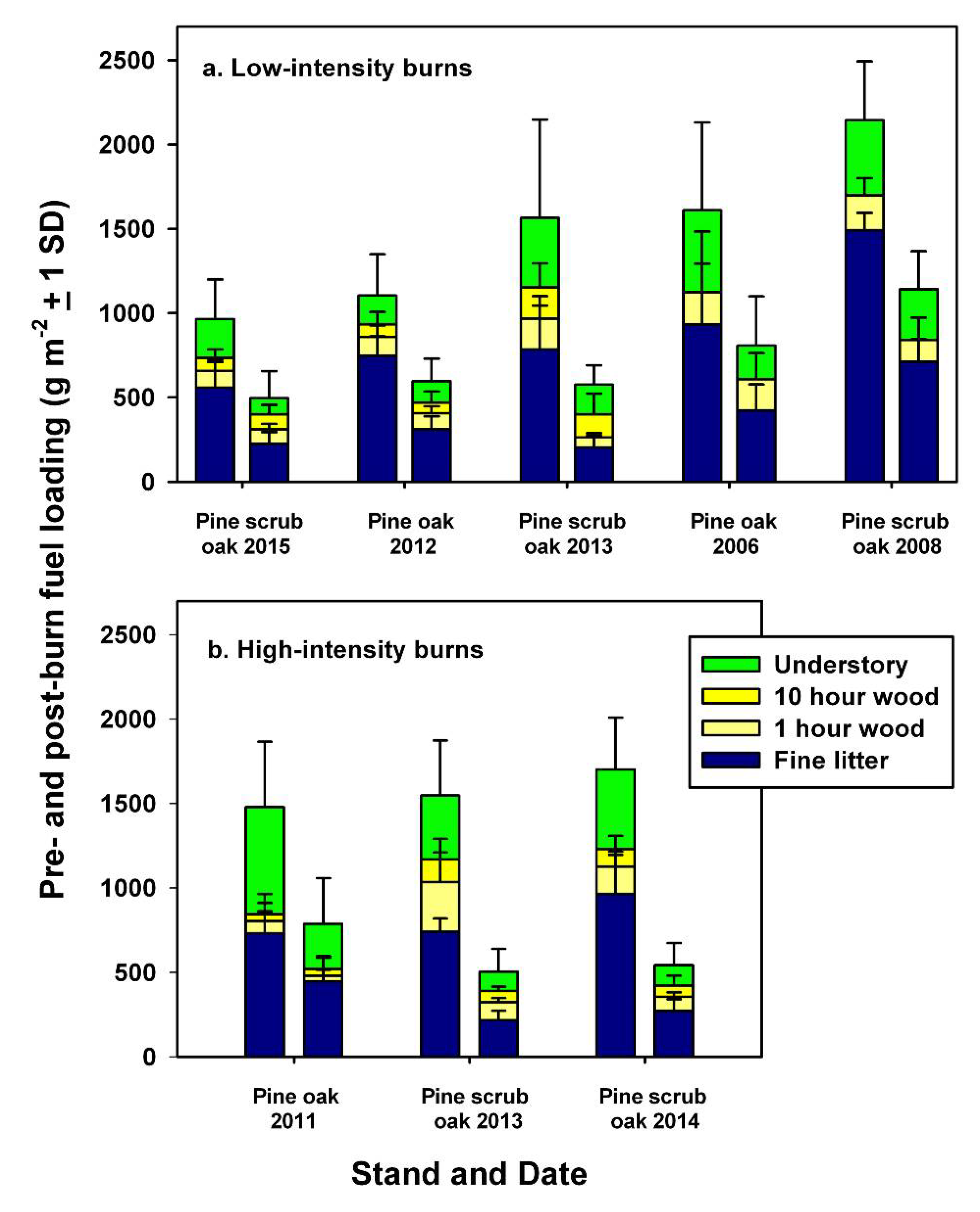
Uncertainty in the estimation of fuel consumption from destructively harvested plots pre- and post-burn was dependent on fuel type. When variation in pre-loading measurements for all stands were considered together, the coefficient of variation (CV; standard deviation/mean) for fine fuels on the forest floor averaged only 26 ± 8%, while the CV for understory vegetation averaged 74 ± 22%, reflecting the increased spatial variability in shrub and scrub oak distribution at a 1 m scale. A second potential source of error was the omission of char particles < 2 mm diameter that were produced during combustion of the forest floor, because we sifted many of the forest floor samples through 2 mm mesh size screens to remove sand and finer, undifferentiated organic matter derived from the uncombusted forest floor material in the O horizon. Despite these potential measurement errors, pre- and post-burn fuel loadings reported here are within the range of previously measured fuel loads on the forest floor, understory, and canopy in the Pinelands National Reserve [23,35,37,38]. Average values for pre- and post-burn fuel loading reported here are slightly lower than in previously measured pine–oak and pitch pine–scrub oak stands burned at typical intervals in the PNR (

Table A5. Pre- and post-burn fuel loading and percent consumption of each fuel type in pine–oak and pine–scrub oak forests in the Pinelands National Reserve. Values are (g m⁻² ± 1 SD), adapted from Clark et al. [23].

Fuel Type	This Study			Average 1
	Pre-Burn	Post-Burn	Percent Consumed	Pre-Burn	Post-Burn	Percent Consumed
	g m−2 ± 1 SD			g m−2 ± 1 SD
Understory	403 ± 147	175 ± 76	56	606 ± 245	267 ± 134	56
Fine litter	869 ± 282	351 ± 172	60	1011 ± 214	482 ± 136	52
1 + 10 hour wood	242 ± 106	156 ± 39	36	230 ± 109	148 ± 56	36
Total	1514 ± 361	682 ± 221	55	1847 ± 240	897 ± 135	52

¹ Values are from n = 25 prescribed fires in pine–oak and pine–scrub oak stands in the PNR; pre-burn surface fuels ranged between 530 ± 210 g m⁻² and 2338 ± 600 g m⁻², and understory vegetation ranged between <150 g m⁻² 1174 ± 398 g m⁻² in frequently-burned stands and a pitch pine–scrub oak stand that had not burned for 47 years, respectively.

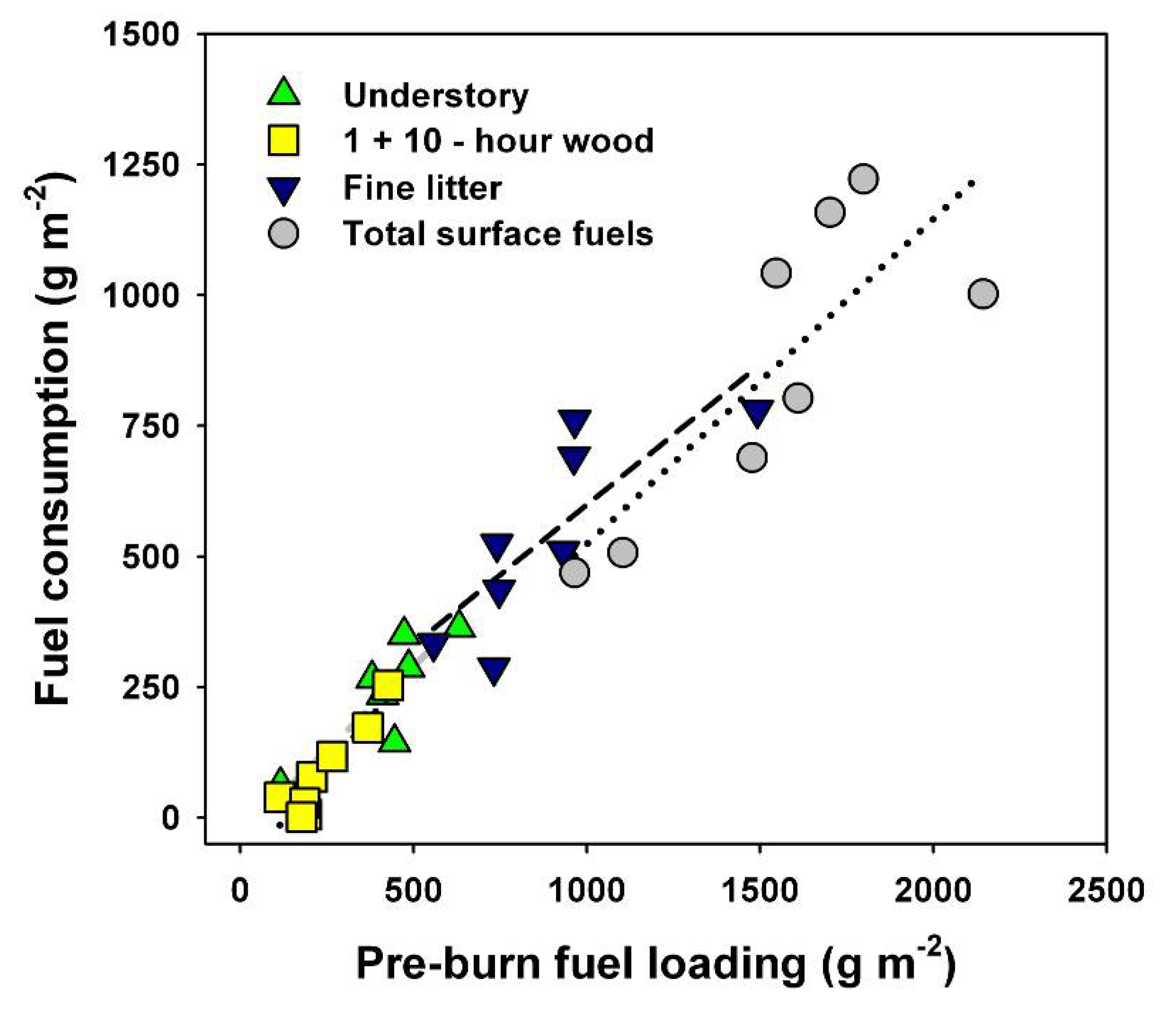
; data from [23]). Fuel consumption estimated for the prescribed burns reported here is within the range of values reported by Clark et al. [23] for 25 prescribed burns in the PNR, where fuel consumption also was a strong linear relationship of initial fuel loading (Table A5). In these previous analyses, initial loading explained 70%, 76% and 73% of the variation in consumption of fine fuels on the forest floor, 1 h + 10 h woody fuels on the forest floor, and understory vegetation, respectively. Significant linear relationships between surface and understory fuel loading and consumption have also been demonstrated at the plot scale for individual fires [36] and across a wider range of fire intensities, including wildfires, in the PNR [29].

The use of sonic anemometers in eddy covariance systems in the fire environment can also result in potential sources of error, primarily because of difficulties in accurately quantifying air temperature and turbulence in buoyant plumes during fire front passage (e.g., [24,49]). Pre- and post-burn measurements in burn areas and all measurements at control towers likely characterized turbulence and energy fluxes reasonably well. Long-term energy flux measurements made pre- and post-prescribed fire using identical instrumentation at three of the burned stands (Fort Dix, Cedar Bridge, and Silas Little Experimental Forest) indicate that half hourly sensible and latent heat fluxes accounted for 93% to 98% of the sum of net radiation, soil heat flux, and heat storage terms in the canopy air space and in biomass [39]. However, sonic anemometers operating at 10 Hz may underestimate instantaneous fluxes during enhanced turbulence occurring at higher frequencies in buoyant plumes during fire front passage [50]. 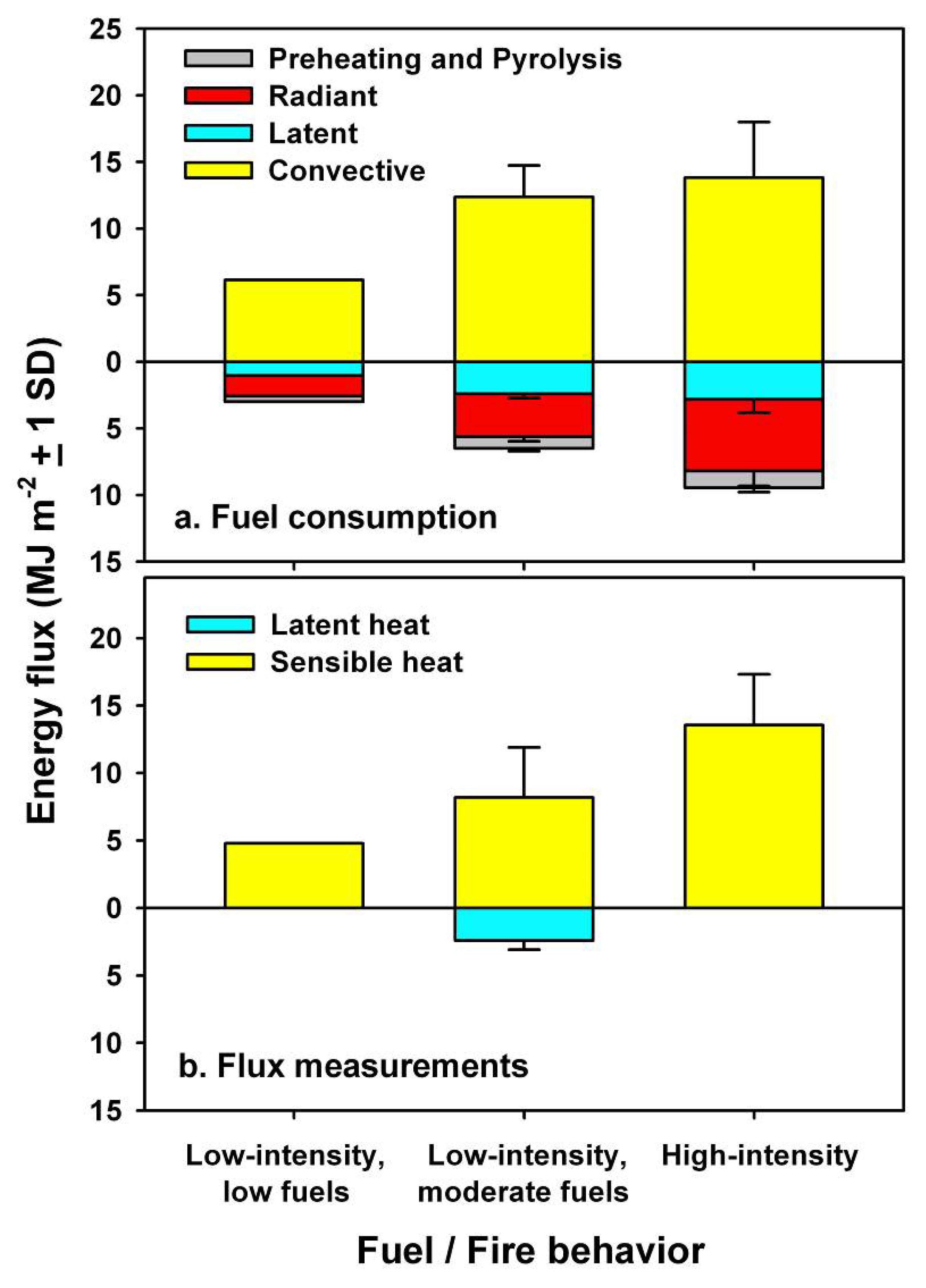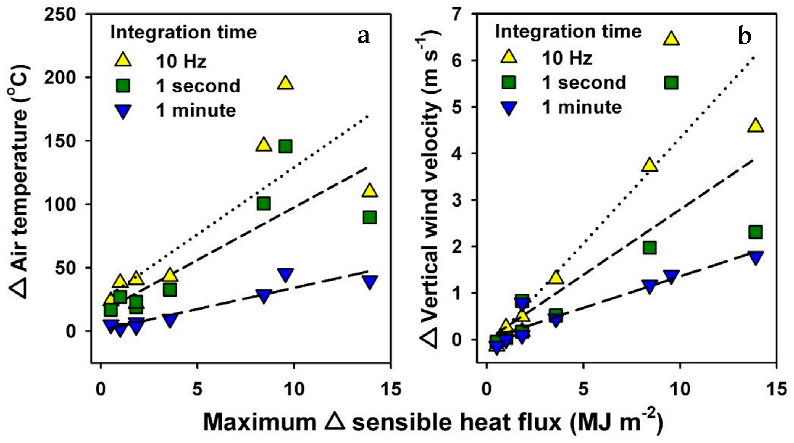Additional uncertainty may arise because flux measurements sample only a limited portion of the flame front, thus the distribution of fire intensities may not be completely captured in the footprint sampled by tower-mounted sensors, especially during high-intensity head fires (e.g., [36]). This is likely one of the reasons that mismatches occur between convective heat fluxes estimated from fuel consumption and integrated Δ sensible heat fluxes shown in Figure 4. During high-intensity head fires, crowning activity in the vicinity of burn area towers led to relatively high values for Δ sensible heat flux values compared to convective heat fluxes calculated from burn area-averaged fuel consumption estimates; when low-intensity versus high-intensity fires were compared, average integrated Δ sensible heat flux values were 70 ± 17% vs. 112 ± 42% of estimated convective heat fluxes, respectively. This result highlights the importance of quantifying the relationships between fire behavior, especially rate of spread and residence time of low-intensity fires, fine-scale measurements of fuel loading and consumption, and their linkage to turbulence and energy flux footprints in future investigations. Additional heat storage in the canopy airspace, in biomass, unconsumed forest floor material, and in soil likely accounted for much of the remaining energy during low-intensity fires. Tower-based measurements of Δ latent heat fluxes did account for nearly all of the estimated latent heat calculated from biometric and fuel moisture measurements during three of the low-intensity fires. We also found that smoke particles occasionally interfered with the sonic anemometer sensor heads, and air temperatures associated with buoyant plumes were occasionally out of range of equipment specifications. In the high-intensity head fires with some crown torching conducted at Warren Grove in 2013 and 2014, two of the sonic anemometers were damaged during fire front passage, but the closely associated thermocouples were not impacted. Thus, some important information could not be collected. Future investigations would benefit from more robust sonic anemometers operating at higher sampling frequencies.

A third source of uncertainty arises from the accurate assessment of ambient conditions during the prescribed fires. Often, ambient conditions are inferred from pre- and/or post-burn measurements from the same tower that the sampled the fire, assuming that conditions were similar to those during the fire event (e.g., [15,25,49]). In this study, we attempted to reduce this potential source of error by using data from independent control towers, and calculated Δ air temperatures, Δ turbulence statistics, and Δ energy fluxes over time periods sampled simultaneously. However, sensor separation due to distances between burn area and control towers also likely influenced all Δ values because different local environments can have substantially different turbulence characteristics. Additionally, during the high-intensity fire conducted near Warren Grove in 2014, it is possible that the control tower may have been influenced by turbulence generated by the high-intensity fire because of its relatively close position on the landscape [36].

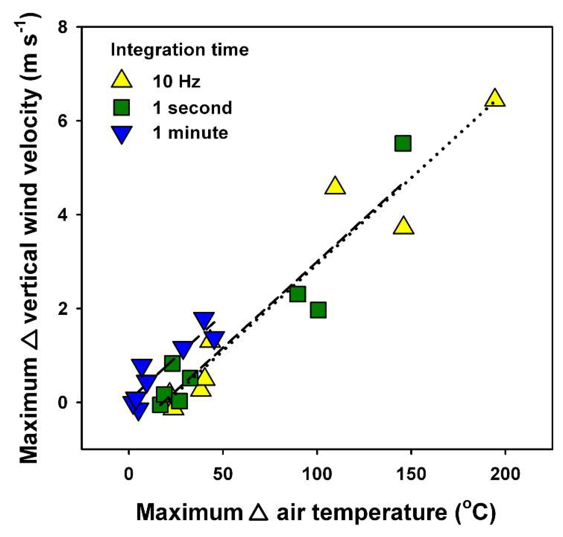
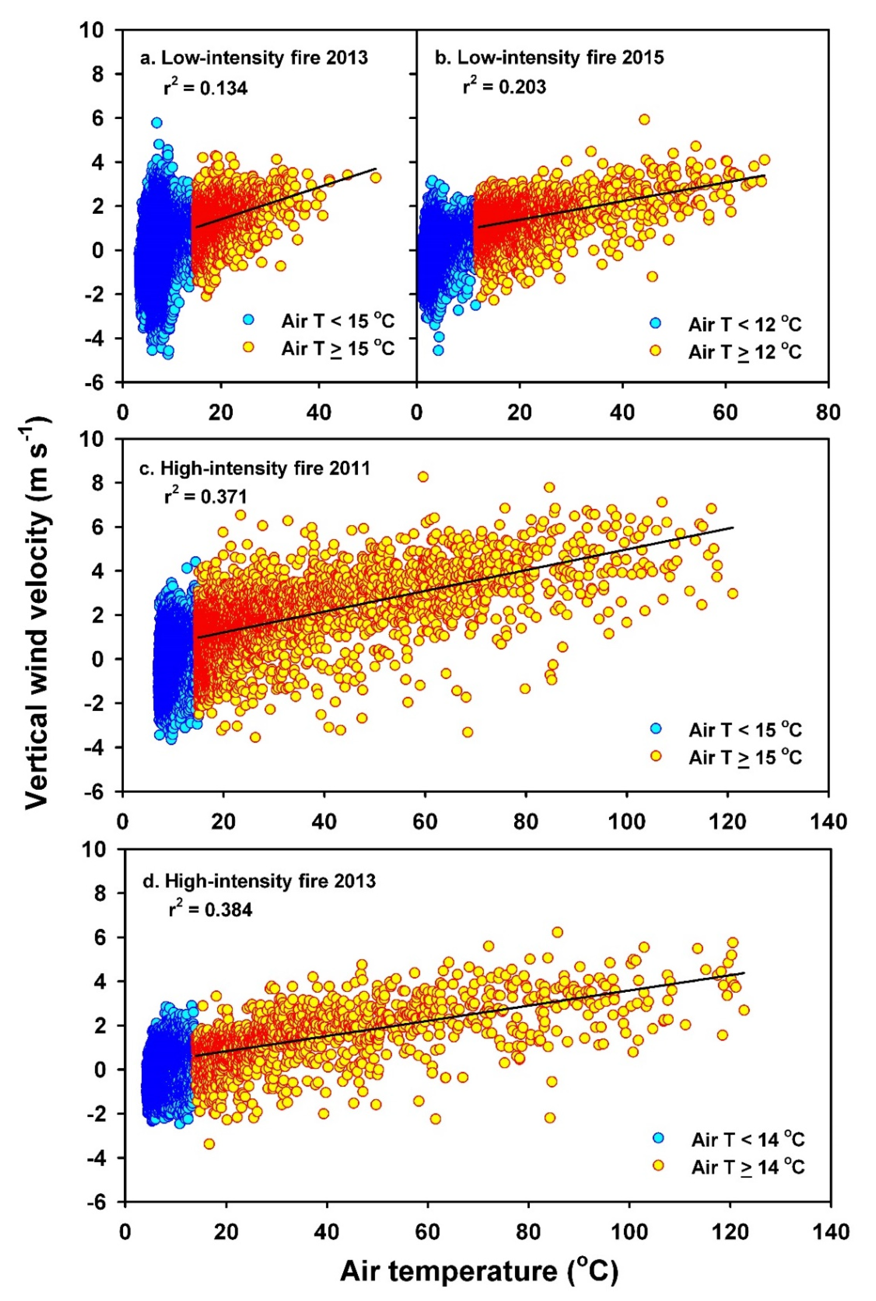
Despite these potential methodological limitations, several recent investigations have used similar suites of eddy covariance and meteorological instrumentation and data reduction techniques to successfully quantify turbulence and energy fluxes in the fire environment (e.g., [15,24,49]). Previous analyses by Heilman et al. [15,25] using profile data from the prescribed fires conducted in 2011 and 2012 analyzed here document how fire front passage modifies the structure of wind fields within and above the canopy, with greatest vertical and horizontal wind perturbations occurring just above the canopy. They also show that horizontal wind velocities associated with buoyant plumes can exceed vertical wind velocities and discuss the importance of interactions between fire front passage and canopy structure in altering patterns of turbulent transfer in buoyant plumes. Recent analyses indicate that the slopes of the relationship between air temperature and vertical wind velocity in buoyant plumes above flame fronts increase significantly with height above the ground. For the 2011 prescribed fire in a pine–oak stand reported here, slopes of this relationship were 0.018, 0.028 and 0.048 at 3, 10 and 20 m measurement heights, respectively. We have observed similar increases in slopes of these relationships with height above flame fronts in a range of experiments where sonic anemometers were arranged in vertical profiles. Clements et al. [24] also indicate that even during low-intensity fires, fire-atmosphere interactions significantly modify turbulence structure and energy fluxes. Convective heating associated with buoyant plumes during fire front passage during their measurements resulted in a peak 1 minute heat flux of 15.2 kW m⁻² during a low-intensity flanking fire during the RxCadre campaign. For comparison, we measured peak 10 minute values of 3.6, 2.8 and 18.0 kW m⁻² during low-intensity fires with low fuel loading, low-intensity fires with moderate fuel loading, and high-intensity fires, respectively.

Quantifying turbulence and energy fluxes across a range of fire intensities during operational fuel reduction treatments will contribute to the development of more robust and accurate tools for predicting fire behavior and smoke dispersion from prescribed fires (e.g., [14,15,16,25,46]). Computationally intensive, physics based models for simulating fuel combustion and fire behavior (e.g., Wildland Urban Interface Fire Dynamics Simulator (WFDS); [51,52], FIRETEC; [53] and QUIC-Fire; [46]), explicitly account for the processes driving fire behavior by coupling and scaling individual component processes at the fuel bed and fire scales with interactions between ambient wind fields, forest structure, and buoyancy- and shear-induced turbulence on the scale of a fire’s plume. Smoke emission and dispersion models (e.g., ARPS-CANOPY/FLEXPART and the BLUESKY modeling framework [14,47,48,54]) couple estimates of fuel consumption and particulate emissions with Lagrangian transport models, and account for characteristics of the forest canopy and how it affects fire-induced turbulence within and above vegetation layers to simulate smoke concentrations during low- and high-intensity fires. A number of model predictions can be evaluated using micrometeorological data collected during fires, but large-scale field experiments such as those reported here have only recently been conducted frequently enough to provide sufficient information to evaluate detailed relationships between ignition pattern and fire behavior, fuel consumption and turbulence and energy fluxes in the fire environment. Continuation of multi-scale experiments that couple above- and within-canopy turbulence and energy flux measurements with more precise measurements of fuel combustion physics such as those conducted under the Department of Defense-sponsored Strategic Environmental Research Program (SERDP) [55] and the multi-agency Fire and Smoke Model Evaluation Experiment (FASMEE) [56] will add considerably to these efforts.

5. Conclusions

Eight prescribed fires were conducted to evaluate the interactions between fire behavior (backing vs. head fires) and initial fuel loading on fuel consumption and above-canopy turbulence and energy fluxes. Forest floor and understory vegetation comprised the majority of consumed fuels, and consumption was significantly correlated with initial loading and less affected by ignition pattern and fire behavior. Consumption of ladder and canopy fuels only occurred during high-intensity head fires, and these fires were associated with enhanced turbulent transfer of smoke and the production and transport of firebrands above the canopy. Above-canopy buoyant heating and turbulence statistics were highly correlated across fires, with highest values occurring in high-intensity head fires. When integrated for the duration of each prescribed fire, above-canopy Δ sensible heat fluxes were similar to convective heat flux values calculated from consumed fuels for low-intensity fires, assuming that some heat was partitioned into soil heat flux and heat storage in the canopy air space and unconsumed biomass. For the high-intensity fires, above-canopy Δ sensible heat fluxes exceeded convective heat flux values, likely due to mismatches between flux footprints and fuel consumption estimates that were averaged across the burn area. There was little relationship between the consumption of surface and understory fuels and buoyant heating or turbulence statistics, indicating that longer residence times of flame fronts during lower intensity backing fires contributed to their effectiveness in reducing surface and understory fuels. These results highlight the importance of quantifying and understanding the relationships between fire behavior, especially rate of spread and residence time of flame fronts, fine-scale measurements of fuel loading and consumption, and turbulence and energy flux footprints in future investigations. Overall, these efforts can assist wildland fire managers optimize hazardous fuel reduction goals while minimizing adverse local air-quality impacts and firebrand production when planning and conducting prescribed fires. Our research also provides valuable turbulence and energy flux data that contribute to the development and evaluation of next-generation fire behavior and smoke dispersion models.

References

1. Agee, J.K.; Skinner, C.N. Basic principles of forest fuel reduction treatments. For. Ecol. Manag. 2005, 211, 83–96. [Google Scholar] [CrossRef]
2. Ryan, K.C.; Knapp, E.E.; Varner, J.M. Prescribed fire in North American forests and woodlands: History, current practice, and challenges. Front. Ecol. Environ. 2013, 11, e15–e24. [Google Scholar] [CrossRef]
3. Addington, R.N.; Hudson, S.J.; Hiers, J.K.; Hurteau, M.D.; Hutcherson, T.F.; Matusick, G.; Parker, J.M. Relationships among wildfire, prescribed fire, and drought in a fire-prone landscape in the south-eastern United States. Int. J. Wildland Fire 2015, 24, 778–783. [Google Scholar] [CrossRef] [Green Version]
4. National Interagency Fire Center. 2019. Available online: https://www.nifc.gov/fireinfo/fireinfo_statistics.html (accessed on 15 October 2019).
5. Little, S.; Allen, J.P.; Moore, E.B. Controlled burning as a dual-purpose tool of forest management in New Jersey’s pine region. J. For. 1948, 46, 810–819. [Google Scholar] [CrossRef]
6. Mitchell, R.J.; Hiers, J.K.; O’Brien, J.J.; Jack, S.B.; Engstrom, R.T. Silviculture that sustains: The nexus between silviculture, frequent prescribed fire, and conservation of biodiversity in longleaf pine forests of the southeastern United States. Can. J. For. Res. 2006, 36, 2724–2736. [Google Scholar] [CrossRef] [Green Version]
7. Hutchinson, T.F.; Long, R.P.; Rebbeck, J.; Sutherland, E.K.; Yaussy, D.A. Repeated prescribed fires alter gap-phase regeneration in mixed-oak forests. Can. J. For. Res. 2012, 42, 303–314. [Google Scholar] [CrossRef]
8. Brose, P.H. Development of prescribed fire as a silvicultural tool for the upland oak forests of the eastern United States. J. For. 2014, 112, 525–533. [Google Scholar] [CrossRef]
9. Kirkman, L.K.; Giencke, L.M.; Taylor, R.S.; Boring, L.R.; Staudhammer, C.L.; Mitchell, R.J. Productivity and species richness in longleaf pine woodlands: Resource-disturbance influences across an edaphic gradient. Ecology 2016, 97, 2259–2271. [Google Scholar] [CrossRef]
10. Dell, J.E.; Richards, L.A.; O’Brien, J.J.; Loudermilk, E.L.; Hudak, A.T.; Pokswinski, S.M.; Bright, B.C.; Hiers, J.K.; Williams, B.W.; Dyer, L.A. Overstory-derived surface fuels mediate plant species diversity in frequently burned longleaf pine forests. Ecosphere 2017, 8. [Google Scholar] [CrossRef]
11. Kelly, L.T.; Brotons, L. Using fire to promote biodiversity. Science 2017, 355, 1264–1265. [Google Scholar] [CrossRef]
12. Nowak, J.T.; Meeker, J.R.; Coyle, D.R.; Steiner, C.A.; Brownie, C. Southern Pine Beetle Infestations in Relation to Forest Stand Conditions, Previous Thinning, and Prescribed Burning: Evaluation of the Southern Pine Beetle Prevention Program. J. For. 2015, 113, 454–462. [Google Scholar] [CrossRef] [Green Version]
13. Dodds, K.J.; Aoki, C.F.; Arango-Velez, A.; Cancelliere, J.; D’Amato, A.W.; DiGirolomo, M.F.; Rabaglia, R.J. Expansion of southern pine beetle into northeastern forests: Management and impact of a primary bark beetle in a new region. J. For. 2018, 116, 178–191. [Google Scholar] [CrossRef] [Green Version]
14. Kiefer, M.T.; Heilman, W.E.; Zhong, S.; Charney, J.J.; Bian, X.; Skowronski, N.S.; Hom, J.L.; Clark, K.L.; Patterson, M.; Gallagher, M.R. Multiscale Simulation of a Prescribed Fire Event in the New Jersey Pine Barrens using ARPS-CANOPY. J. Appl. Meteorol. Climatol. 2014, 53, 793–812. [Google Scholar] [CrossRef]
15. Heilman, W.E.; Clements, C.B.; Seto, D.; Bian, X.; Clark, K.L.; Skowronski, N.S.; Hom., J.L. Observations of fire-induced turbulence regimes during low-intensity wildland fires in forested environments: Implications for smoke dispersion. Atmos. Sci. Lett. 2015, 16, 453–460. [Google Scholar] [CrossRef] [Green Version]
16. Navarro, K.; Schweizer, D.; Balmes, J.; Cisneros, R. A Review of Community Smoke Exposure from Wildfire Compared to Prescribed Fire in the United States. Atmosphere 2018, 9, 185. [Google Scholar] [CrossRef] [Green Version]
17. Scott, J.; Burgan, R. Standard Fire Behavior Fuel Models: A Comprehensive Set for Use with Rothermel’s Surface Fire Spread Model; General Technical Report RMRS-GTR-153; USDA Forest Service, Rocky Mountain Research Station: Fort Collins, Colorado, USA, 2005; 72p. [Google Scholar]
18. Ottmar, R.D.; Blake, J.I.; Crolly, W.T. Using fine-scale fuel measurements to assess wildland fuels, potential fire behavior and hazard mitigation treatments in the southeastern USA. For. Ecol. Manag. 2012, 273, 1–3. [Google Scholar] [CrossRef]
19. Ottmar, R.D.; Hudak, A.T.; Prichard, S.J.; Wright, C.S.; Restaino, J.C.; Kennedy, M.C.; Vihnanek, R.E. Pre-fire and post-fire surface fuel and cover measurements collected in the south-eastern United States for model evaluation and development–RxCADRE 2008, 2011 and 2012. Int. J. Wildland Fire 2016, 25, 10–24. [Google Scholar] [CrossRef]
20. Potter, B.E. Atmospheric interactions with wildland fire behaviour–I. Basic surface interactions, vertical profiles and synoptic structures. Int. J. Wildland Fire 2012, 21, 779–801. [Google Scholar] [CrossRef]
21. Martin, R.A.; Hamman, S.T. Ignition patterns influence fire severity and plant communities in Pacific Northwest, USA, prairies. Fire Ecol. 2016, 12, 88–102. [Google Scholar] [CrossRef] [Green Version]
22. Reid, A.M.; Robertson, K.M.; Hmielowski, T.L. Predicting litter and live herb fuel consumption during prescribed fires in native and old-field upland pine communities of the southeastern United States. Can. J. For. Res. 2012, 42, 1611–1622. [Google Scholar] [CrossRef]
23. Clark, K.L.; Skowronski, N.; Gallagher, M. Fire management and carbon sequestration in Pine Barren forests. J. Sustain. For. 2015, 34, 125–146. [Google Scholar] [CrossRef]
24. Clements, C.B.; Lareau, N.P.; Seto, D.; Contezac, J.; Davis, B.; Teske, C.; Zajkowski, T.J.; Hudak, A.T.; Bright, B.C.; Dickinson, M.B.; et al. Fire weather conditions and fire–atmosphere interactions observed during low-intensity prescribed fires–RxCADRE 2012. Int. J. Wildland Fire 2016, 25, 90–101. [Google Scholar] [CrossRef]
25. Heilman, W.E.; Bian, X.; Clark, K.L.; Skowronski, N.S.; Hom, J.L.; Gallagher, M.R. Atmospheric Turbulence Observations in the Vicinity of Surface Fires in Forested Environments. J. Appl. Meteorol. Climatol. 2017, 56, 3133–3150. [Google Scholar] [CrossRef]
26. Clark, K.L.; Skowronski, N.; Hom, J.; Duveneck, M.; Pan, Y.; Van Tuyl, S.; Cole, J.; Patterson, M.; Maurer, S. Decision support tools to improve the effectiveness of hazardous fuel reduction treatments in the New Jersey Pine Barrens. Int. J. Wildland Fire 2009, 18, 268–277. [Google Scholar] [CrossRef]
27. La Puma, I.P.; Lathrop, R.G., Jr.; Keuler, N.S. A large-scale fire suppression edge-effect on forest composition in the New Jersey Pinelands. Landsc. Ecol. 2013, 28, 1815–1827. [Google Scholar] [CrossRef]
28. Skowronski, N.S.; Haag, S.; Trimble, J.; Clark, K.L.; Gallagher, M.R.; Lathrop, R.G. Structure-level fuel load assessment in the wildland–urban interface: A fusion of airborne laser scanning and spectral remote-sensing methodologies. Int. J. Wildland Fire 2016, 25, 547–557. [Google Scholar] [CrossRef]
29. Gallagher, M.R. Monitoring Fire Effects in the New Jersey Pine Barrens with Burn Severity Indices. Ph.D. Thesis, Rutgers University, New Brunswick, NJ, USA, 2017; p. 146. [Google Scholar] [CrossRef]
30. Little, S.; Moore, E.B. The ecological role of prescribed burns in the pine-oak forests of southern New Jersey. Ecology 1949, 30, 223–233. [Google Scholar] [CrossRef]
31. Forman, R.T.T.; Boerner, R. Fire frequency and the Pine Barrens of New Jersey. Bull. Torrey Bot. Club 1981, 108, 34–50. [Google Scholar] [CrossRef]
32. State Climatologist of New Jersey Climate Data. Available online: https://climate.rutgers.edu/stateclim/ (accessed on 15 November 2018).
33. Pan, Y.; Birdsey, R.; Hom, J.; McCullough, K.; Clark, K. Improved estimates of net primary productivity from MODIS satellite data at regional and local scales. Ecol. Appl. 2006, 16, 125–132. [Google Scholar] [CrossRef]
34. Clark, K.L.; Renninger, H.J.; Skowronski, N.; Gallagher, M.; Schäfer, K.V.R. Decadal-scale reduction in forest net ecosystem production following insect defoliation contrasts with short-term impacts of prescribed fires. Forests 2018, 9, 145. [Google Scholar] [CrossRef] [Green Version]
35. Wright, C.S.; Ottmar, R.D.; Vihnanek, R.E. Stereo photo series for quantifying natural fuels. In Hardwood, Pitch Pine, and Red Spruce/Balsam Fir types in the Northeastern United States PMS 840; National Wildfire Coordinating Group, National Interagency Fire Center: Boise, ID, USA, 2007; Volume VIII, 91p. [Google Scholar]
36. Mueller, E.V.; Skowronski, N.; Clark, K.; Gallagher, M.; Kremens, R.; Thomas, J.C.; El Houssami, M.; Filkov, A.; Hadden, R.M.; Mell, W.; et al. Utilization of remote sensing techniques for the quantification of fire behavior in two pine stands. Fire Saf. J. 2017, 91, 845–854. [Google Scholar] [CrossRef] [Green Version]
37. Skowronski, N.S.; Clark, K.L.; Duveneck, M.; Hom, J. Three-dimensional canopy fuel loading predicted using upward and downward sensing LiDAR systems. Remote Sens. Environ. 2011, 115, 703–714. [Google Scholar] [CrossRef]
38. Clark, K.L.; Skowronski, N.; Gallagher, M.; Carlo, N.; Farrell, M.; Maghirang, M.R. Assessment of canopy fuel loading across a heterogeneous landscape using LiDAR. In Joint Fire Sciences Program Project Final Report, 10-1-02-14; Joint Fire Science Program: Boise, ID, USA, 2013. [Google Scholar]
39. Clark, K.L.; Skowronski, N.; Gallagher, M.; Renninger, H.; Schäfer, K. Effects of invasive insects and fire on forest energy exchange and evapotranspiration in the New Jersey pinelands. Agric. For. Meteorol. 2012, 166, 50–61. [Google Scholar] [CrossRef]
40. Kremens, R.L.; Dickinson, M.B.; Bova, A.S. Radiant flux density, energy density and fuel consumption in mixed-oak forest surface fires. Int. J. Wildland Fire 2012, 21, 722–730. [Google Scholar] [CrossRef]
41. Clement, R. EdiRe Data Software, Version 1.5. 0.32; University of Edinburgh: Edinburgh, UK, 2012. [Google Scholar]
42. Winter, G.J.; Vogt, C.; Fried, J.S. Fuel treatments at the wildland-urban interface: Common concerns in diverse regions. J. For. 2002, 100, 15–21. [Google Scholar] [CrossRef]
43. Mell, W.E.; Manzello, S.L.; Maranghides, A.; Butry, D.; Rehm, R.G. The wildland–urban interface fire problem–current approaches and research needs. Int. J. Wildland Fire 2010, 19, 238–251. [Google Scholar] [CrossRef]
44. Filkov, A.; Prohanov, S.; Mueller, E.; Kasymov, D.; Martynov, P.; El Houssami, M.; Thomas, J.; Skowronski, N.; Butler, B.; Gallagher, M.; et al. Investigation of firebrand production during prescribed fires conducted in a pine forest. Proc. Combust. Inst. 2017, 36, 3263–3270. [Google Scholar] [CrossRef]
45. Thomas, J.C.; Mueller, E.V.; Santamaria, S.; Gallagher, M.; El Houssami, M.; Filkov, A.; Clark, K.; Skowronski, N.; Hadden, R.M.; Mell, W.; et al. Investigation of firebrand generation from an experimental fire: Development of a reliable data collection methodology. Fire Saf. J. 2017, 91, 864–871. [Google Scholar] [CrossRef] [Green Version]
46. Linn, R.R.; Goodrick, S.L.; Brambilla, S.; Brown, M.J.; Middleton, R.S.; O’Brien, J.J.; Hiers, J.K. QUIC-fire: A fast-running simulation tool for prescribed fire planning. Environ. Model. Softw. 2020, 125, 104616. [Google Scholar] [CrossRef]
47. Kiefer, M.T.; Zhong, S.; Heilman, W.E.; Charney, J.J.; Bian, X. Evaluation of an ARPS-based canopy flow modeling system for use in future operational smoke prediction efforts. J. Geophys. Res. Atmos. 2013, 118, 6175–6188. [Google Scholar] [CrossRef]
48. Charney, J.J.; Kiefer, M.T.; Zhong, S.; Heilman, W.E.; Nikolic, J.; Bian, X.; Hom, J.L.; Clark, K.L.; Skowronski, N.S.; Gallagher, M.R.; et al. Assessing forest overstory impacts on smoke concentrations using a coupled numerical model. Atmosphere 2019, 10, 273. [Google Scholar] [CrossRef] [Green Version]
49. Seto, D.; Clements, C.B.; Heilman, W.E. Turbulence spectra measured during fire front passage. Agric. For. Meteorol. 2013, 169, 195–210. [Google Scholar] [CrossRef]
50. Frankman, D.; Webb, B.W.; Butler, B.W.; Jimenez, D.; Forthofer, J.M.; Sopko, P.; Shannon, K.S.; Hiers, J.K.; Ottmar, R.D. Measurements of convective and radiative heating in wildland fires. Int. J. Wildland Fire 2013, 22, 157–167. [Google Scholar] [CrossRef]
51. Mell, W.; Maranghides, A.; McDermott, A.; Manzello, S.L. Numerical simulation and experiments of burning douglas fir trees. Combust. Flame 2009, 156, 2023–2041. [Google Scholar] [CrossRef]
52. Mueller, E.; Mell, W.; Simeoni, A. Large eddy simulation of forest canopy flow for wildland fire modeling. Can. J. For. Res. 2014, 44, 1534–1544. [Google Scholar] [CrossRef]
53. Linn, R.; Reisner, J.; Colman, J.J.; Winterkamp, J. Studying wildfire behavior using FIRETEC. Int. J. Wildland Fire 2002, 11, 233–246. [Google Scholar] [CrossRef]
54. Larkin, N.K.; O’Neill, S.M.; Solomon, R.; Raffuse, S.; Strand, T.; Sullivan, D.; Krull, C.; Rorig, M.; Peterson, J.; Ferguson, S.A. The BlueSky smoke modeling framework. Int. J. Wildland Fire 2009, 18, 906–920. [Google Scholar] [CrossRef] [Green Version]
55. Skowronksi, N. Multi-Scale Analyses of Wildland Fire Combustion Processes in Open-Canopied Forests Using Coupled and Iteratively Informed Laboratory-, Field-, and Model-Based Approaches. Available online: https://www.serdp-estcp.org/Program-Areas/Resource-Conservation-and-Resiliency/Air-Quality/RC-2641 (accessed on 15 November 2019).
56. Prichard, S.; Larkin, N.S.; Ottmar, R.; French, N.H.; Baker, K.; Brown, T.; Clements, C.; Dickinson, M.; Hudak, A.; Kochanski, A.; et al. The Fire and Smoke Model Evaluation Experiment—A Plan for Integrated, Large Fire–Atmosphere Field Campaigns. Atmosphere 2019, 10, 66. [Google Scholar] [CrossRef] [Green Version]
Figure 1. Examples of fire behavior during the eight prescribed fires conducted in the New Jersey Pinelands National Reserve. (a) low-intensity backing fire in a pine–oak stand at the Silas Little Experimental Forest in 2012; (b) low-intensity backing fire in a pitch pine–scrub oak stand near the Cedar Bridge fire tower in 2013; note the eddy flux tower in the background; (c) high-intensity head fire initiating crown torching in a pitch pine–scrub oak stand near Warren Grove in 2014, and (d) one of the flux towers following a high-intensity head fire near Warren Grove in 2014.
Atmosphere 11 00242 g001
Figure 2. Pre- and post-burn fuel loading for the eight prescribed fires, partitioned into understory, 1 hour and 10 hour wood, and fine litter. Fuel loadings are presented for (a) low-intensity burns and (b) high-intensity burns. Table A1 presents source fuel loading values.
Atmosphere 11 00242 g002
Figure 3. The relationship between pre-burn loading and consumption of surface and understory fuels estimated from 1.0 m2 plots (n = 10 to 32 in each burn) for the eight prescribed fires. Linear models and statistics are shown in Table 3, and all data are presented in Table A1. Lines indicate linear models for the relationships between pre-burn loading and consumption for each fuel type and for total surface and understory fuels.
Atmosphere 11 00242 g003
Figure 4. Estimated energy fluxes during the eight prescribed fires, separated by low-intensity fires with relatively low fuel loading, low-intensity fires with moderate fuel loading, and high-intensity fires. (a) Energy release calculated from consumed fuels, partitioned into energy consumed during preheating and pyrolysis of fuels, and radiant, latent, and convective heat fluxes. Values for preheating and pyrolysis of fuels, radiant heat flux and latent heat flux are shown below the zero-line to facilitate comparison between convective and Δ sensible heat fluxes. (b) Δ Sensible and Δ latent heat fluxes calculated from integrated eddy covariance measurements at burn area and control towers. Δ Latent heat fluxes were measured above burn area and control towers at the three low-intensity fires with moderate surface and understory fuels only. Only two low-intensity fires with low fuel loading were conducted thus no error terms are presented.
Atmosphere 11 00242 g004