Abstract
Numerical weather prediction models require an accurate parametrization of the energy budget at the air-ground interface, that can be obtained only through long-term atmospheric boundary layer measurements at different spatial and temporal scales. Despite their importance, such measurements are still scarce even in well-characterized areas. In this paper, a three-year dataset from four micrometeorological stations run by the Regional Agency for Environmental Protection of Lazio was analyzed to estimate albedo, zero-displacement height, roughness length and surface properties over Rome and its suburbs, characterizing differences and interconnections between urban, suburban and rural areas of the same municipality. The integral albedo coefficient at the zenith for the urban station was found to be almost twice that for suburban and rural stations. The zero-displacement height of the urban site was strongly dependent on wind direction, with values varying between 12.0 and 17.8 m, while the roughness length (≈1.5 m) was almost independent of upwind direction, but it was significantly higher than the typical values calculated for rural stations (≈0.4 m). The apparent thermal capacities and thermal conductivity at all the non-urban sites were in fair agreement with each other and typical of soils with relatively low water content, as expected for a relatively dry Mediterranean area like Rome, while the apparent thermal diffusivity reflected the presence of different soil types.
1. Introduction
Although urban areas comprise a very small fraction of Earth’s land cover [1], over half of the global population live in cities, and this percentage is expected to increase in the upcoming decades [2]. Therefore, it is important to monitor, understand, and predict the modifications occurring in local weather and climate due to urbanization, particularly in the perspective of accurate high-resolution weather and air-quality forecasting and climate-sensitive urban design and planning.
Cities are characterized by a high fraction of impervious surfaces, which modify both surface energy and water balances affecting both the atmospheric boundary layer (ABL) and the weather processes [3]. The presence of large urban agglomerations inevitably generates deep disturbances in the dynamic and thermodynamic characteristics of the ABL, leading to a higher air pollution concentration in winter and enhanced heat wave impact in summer [4].
In order to monitor and predict the levels of pollution and the distribution of air temperature near the ground, prognostic meteorological models (NWP) and photochemical models are routinely used [5]. The combination of the two models is also the heart of near real-time systems which, by assimilating meteorological, micrometeorological and atmospheric pollutant concentration measurements, provide the most probable spatial representation of the phenomena. The essential requirement for a realistic forecast model is to be able to properly reconstruct the dynamic and thermodynamic characteristics of the ABL [6]. It is well known [7,8,9] that such a capability mostly depends on the reliability of the parameterizations of the energy and water budget at the air-ground interface. Although the NWPs most used in practical applications have sophisticated schemes for both urban and rural environments, it is not easy to quantify their performances because of a clear lack of long-term ABL observations [6]. Long-term urban ABL observations at different spatial and temporal scales using various instruments have been made just in a few cities [10], mostly without using state-of-the-art techniques. Other studies have focused on specific campaigns, often with less than one year of measurements. So far, urban ABL research has used single- or few-point measurements [11,12,13,14,15,16,17]. Additionally, a reliable urban canopy representation [18] and specification of surface properties is crucial to properly characterize urban forcing, but despite their importance in testing the quality of the model output, which is well recognized by many authors [19], surface property measurements are still scarce. In addition, it is worth noting that an unrealistic characterization of the meteorology in the immediate vicinity of the soil can generate unrealistic meteorological fields even at higher altitudes.
The main objective of the present work was the estimation of albedo, soil thermal properties, roughness length and zero-displacement height, that directly or indirectly characterized the dispersing capacity of the ABL over Rome and its surroundings, by measurements collected in the four locations of the ARPA Lazio micrometeorological network located in the city—one urban station, one sub-urban and two rural. These stations included turbulence and radiation measurements in addition to wind speed and direction, precipitation, pressure, temperature and humidity records. Some of the results about albedo, roughness length and zero-displacement height over three out of the four locations considered in this paper have already been published in [20], and have been reported here for the sake of completeness. Nevertheless, to our knowledge this is the first time that such a dataset was analyzed to estimate soil thermal properties over Rome’s area.
2. Site and Measurements
The area under investigation is Rome, the largest city and the most populated municipality in Italy, located in the central-western part of the country and extending over an area of approximately 5000 km2, with more than four million residents and high-density residential areas located all around the city center. The area is characterized by a complex orography, with the Apennines mountain chain on the eastern side across the Tiber valley. From the southeast and the northeast, the volcanic plateau slopes toward the Tiber from the Alban hills and the Sabatini volcanic fields [21], while Mountains of Tolfa lie to the north. To the southern-eastern side of Rome, a valley separates the Apennines from Alban Hills; the western side of the area is characterized by low land reaching the coastal area, facing the Tyrrhenian sea. Rome is divided by the narrow valley of Tiber, which flows through the city from north to west (Figure 1).
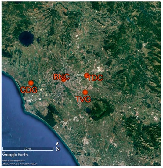
Figure 1.
Location of the ARPA Lazio micro-meteorological network (BNCu, Rome city center; CDGr, Castel di Guido; TVGr, Tor Vergata; TDCs, Tenuta del Cavaliere).
Table 1 reports name, ID, geographical coordinates, altitude above the sea level and classification on the base of the prevailing land use (urban, suburban, rural) for each measuring site. The urban station is located in the historic center of Rome at the top of the building where the ARPA Lazio headquarters (Boncompagni street-urban, hereafter BNCu) is located. The suburban station of Tenuta del Cavaliere (TDCs) is located at the edge of Rome, in an area where vegetated spots, roads and industrial buildings coexist. Tor Vergata (TVGr) and Castel di Guido (hereafter CDGr) can be considered rural. The last two stations, although belonging to the same class, are somehow different: CDGr is close to the Tyrrhenian coast, while that of TVGr is in a rural inland area.

Table 1.
ARPA Lazio micro-meteorological stations.
The instrumental equipment of all the stations allows for the determination of the average values of a number of relevant meteorological and turbulent variables. In particular, the three rural/semirural stations consist of:
- a 10-m meteorological mast having a geometry that minimizes the distortion of the air mass flow;
- an acquisition processing and transmission system, located at the base of the meteorological mast;
- a three-axial ultrasonic anemometer/thermometer (USA 1, Metek, GmbH) and a thermo-hygrometer (HMP45AD, Vaisala) located at the top of the mast, operating at 10 Hz;
- a system for measuring the incident shortwave solar radiation (direct and diffuse), and the atmospheric and terrestrial infrared radiation located near the top of the meteorological mast (CNR 1, Kipp and Zonen).
- a barometer (PTB110 Vaisala), located inside the plastic container that houses the measurement acquisition system;
- a rain gauge placed at the ground close to the meteorological mast;
- a flux plate (HFP01 Hukseflux) at a depth of 5 cm for measuring the vertical heat flux in the ground;
- four thermometers placed in the soil at depths of 2.5 cm, 5 cm, 10 cm and 50 cm, respectively to determine the vertical profile of soil temperature.
The BNCu urban station is identical to the rural stations except that the height of the mast is 6 m above the 23-m rooftop on which it is deployed, and there are no flux plate and thermometers in the ground.
The present study considered three-year measurements, from 2013 to 2015. Anemometer and thermohygrometer measurements were acquired at a frequency of 10 Hz, while the other measurements were acquired at a frequency of 1 Hz.
All retrieved measurements were processed as follows and averaged over a 30-min interval.
- a
- Triaxial ultrasonic anemometer: the Cartesian components of the wind vector acquired at 10 Hz (the x,y,z axes point respectively towards north, east and upwards) and the sonic temperature corresponding to an averaging time of 30 min, compatible with the spectral gap, were considered. The acquisition and processing system applies the Eddy Covariance technique to all the elementary measurements [22,23,24]. After two rotations of the Cartesian axes to bring back the elementary measurements of the motion components to a streamline reference system [25,26], despiking and linear detrending, the system estimates the meteorological and micrometeorological parameters: average wind speed and direction, average virtual temperature, standard deviation of wind speed and direction, standard deviation of longitudinal, transverse and vertical components of motion, standard deviation of virtual temperature, variance-covariance matrix of Reynolds stresses, and covariance between the vertical component of motion and the virtual temperature. From the variance-covariance matrix of the Reynolds stresses and from the covariance between the vertical component of the motion and the virtual potential temperature the friction velocity , the turbulent sensible heat flux H0, the temperature scale , the Monin–Obukhov length L and Turbulent Kinetic Energy TKE are finally estimated [23].
- b
- Thermo-hygrometer: the mean values of the air temperature and relative humidity are calculated from raw data acquired through the analog ports of the sonic anemometer.
- c
- Radiometric system: the radiometric system consists of two pyranometers (to measure the downward and upward solar radiation) and two pyrgeometers (to measure the downward and upward infrared radiation). Once the correction of longwave radiation has been done the average value of global solar radiation (sum of direct and diffuse radiation), reflected solar radiation (albedo), atmospheric infrared radiation and terrestrial infrared radiation is estimated.
- d
- Heat Flux Plate: the average value of the heat flux in the soil is obtained from the raw data produced by the flux plate placed in the soil at a depth of 5 cm. It is worth noting that this estimation does not necessarily represent the flux of heat by conduction, which occurs at the air-ground interface.
- e
- Thermometers in the ground: in each non-urban measurement station four thermometers are placed at 2.5, 5, 10 and 50 cm, respectively. The mean temperature profile is obtained averaging the raw data acquired at each of these four levels.
3. Results
The time series retrieved from the four measuring points described in the previous section allowed for the characterization of the following parameters:
- The integral albedo and its variability with land-use and solar elevation angle, that is crucial to parameterize the surface radiative budget in both urban and rural areas.
- The soil thermal characteristics for rural and suburban sites, the apparent thermal conductivity, the apparent thermal capacity and the apparent thermal diffusivity defined as the ratio of the two. This allows for the estimation of the heat flux G0 at the soil surface. Note that this parameter cannot be measured directly, while it is relatively simple to measure the heat flux into the ground just below the surface. However, it has to be taken into account as the energy budget in urban areas depends not only on the heat flux G0 but also other terms such as the anthropogenic heat and the thermal store of buildings, that cannot be deduced from the available measures [27].
- The roughness length and displacement height parameters that govern the surface exchange of momentum between the atmosphere and the soil.
3.1. Global Albedo
One piece of information required in a NWP model for the correct quantification of the surface radiative budget is the Integral Albedo Coefficient (A), defined as the ratio between the incoming shortwave radiation from the sun (direct and diffuse) and the part reflected from the surface. The coefficient A depends on both the type of reflective surface and the solar elevation angle Ψ, as well as the water content of the soil. In general, given a certain water content and certain optical surface characteristics, A decreases with increasing Ψ values, tending toward an asymptotic value for high values of Ψ. According to [28]:
where a and b are two parameters to which the values 0.1 and 0.5 are generally assigned, respectively, and A0 is the Integral Albedo Coefficient at the zenith.
Figure 2, Figure 3, Figure 4 and Figure 5 show the behavior of A retrieved by Equation (1) as a function of the incident solar radiation (all data were averaged over 2° solar elevation angle intervals, including observations in both clear and cloudy conditions)The integral albedo coefficient decreases with the increase of the solar elevation angle, as foreseen by Equation (1), and its behavior is consistent with that reported in [29], including the scatter of the measurements usually attributed to both a sudden variation of the incident solar radiation (because of the fast passage of cloudy) and/or instrumental noise.
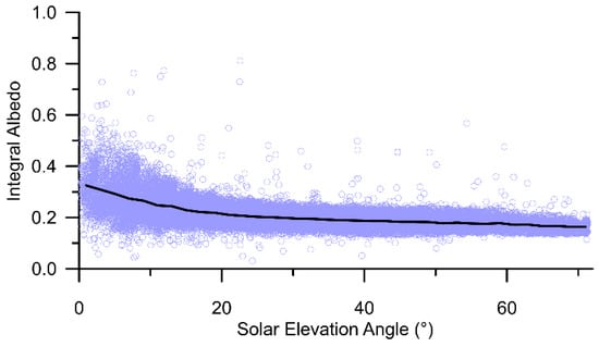
Figure 2.
Integral Albedo for TVGr.
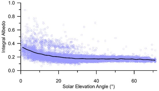
Figure 3.
Integral Albedo for TDCs.
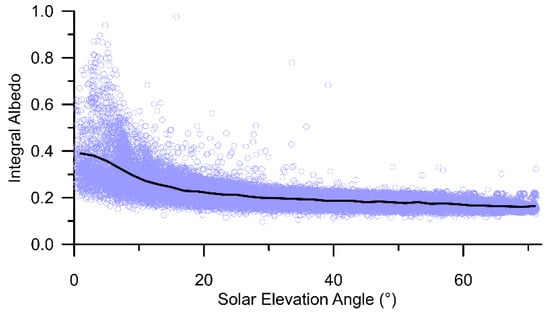
Figure 4.
Integral Albedo for CDGr.
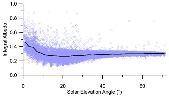
Figure 5.
Integral Albedo for BNCu.
Figure 6 shows the average Integral Albedo Coefficients as a function of the solar elevation angle for all the sites. Similar absolute values and behavior were found for the three non-urban sites, while for BNCu A turned out to be both significantly higher (because of the greater reflectivity of the surroundings surfaces) and less dependent on the solar elevation angle. The observed behavior was suggested to double the value commonly used for a in Equation (1) from 0.1 to 0.2.
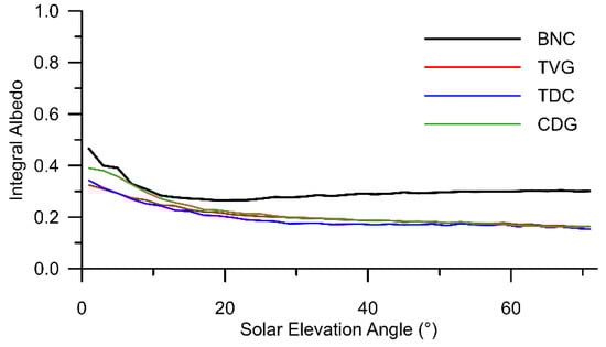
Figure 6.
Integral albedo coefficients as a function of solar elevation angle for all the sites.
In addition, the A value at the zenith (A0) for all sites, defined as the average value of A when the angle of solar elevation was higher than 40°, is listed in Table 2.
Table 2.
Integral Albedo Coefficients at the zenith for all the sites.
For all non-urban stations A0 ≈ 0.16, which was the typical value for a vegetated surface (Tables 11-4 and 11-8 in [30]). On the other hand, the A0 related to the urban station BNCu was almost double. Even if such a result was expected, [29] reports A0 for urban areas to be in the range 0.10–0.27, while in this case the retrieved value was slightly higher than the upper limit of it: this measurement station, unlike typical urban stations considered in most papers, is located within an area completely devoid of vegetation, with concrete buildings of medium height (30-m tall on average) densely packed and a road network structured in deep canyons.
As mentioned in the Introduction, the presented albedo results have to be considered as an integration of what was published in [20].
3.2. Soil Thermal Properties
In the parameterizations used by NWPs, the thermal properties of the soil are crucial to estimating the heat flux at the air-soil interface, the surface temperature of the soil and the vertical distribution of the heat into the ground. Generally, in the NWP models these parameters are tabular values assigned on the basis of the prevailing land-use of the soil, i.e., they are just a rough approximation of real terrain characteristics. The availability of the three-year series of data acquired in Rome’s area allows a more realistic estimate of them, even if the soil water content is not explicitly known.
For the three non-urban micrometeorological stations, the half-hour average values of the vertical heat flux G into the ground at 5 cm and the average temperatures of the ground at 2.5 cm, 5.0 cm, 10 cm and 50 cm were considered. To obtain the value of G at 5 cm, the flux obtained from the plate was corrected to take into account both the difference in thermal capacity between the ground and the material of which the plate was made and its geometry [31,32].
3.2.1. Apparent Soil Thermal Capacity
The process of heat transmission from the air-soil interface into the ground is well known. In general, the prevailing mechanisms are conduction, convection and irradiation. Experimentally, it has been evidenced that the main mechanism of heat transmission is conduction and, if the soil is flat and homogeneous, the transfer of heat from the atmosphere into the ground below is mainly a pure vertical conduction as shown in [33,34]. In Refs. [35,36] the situation in which convection is present but not prevalent has also been considered. Taking into account conduction as the main mechanism, with z on the vertical axis positive downwards and Cs the Apparent Thermal Capacity of the ground, the relationship between G at the depth z and the temperature variation is [33]:
that represents the mathematical representation of the principle of energy conservation at a depth z.
Integrating Equation (2), the value of Cs can be determined as shown in Appendix A.
The thermal capacity computed in this way was representative for a layer of soil between 50 cm and 5 cm. If the soil were completely homogeneous along the vertical, the characterization would be complete. However, the thermal property of soil also depends on its water content, which varies with precipitation. The dataset presented here does not consent to determine such a parameter, but nonetheless Cs can still be estimated assuming it is a stochastic variable whose static properties are summarized in Table 3; which means, in turn, that the provided estimation relies on the assumption that soil water content variation during the three-years is characteristic of the area.
Table 3.
The thermal capacity of the soil Cs for the three non-urban stations. Reference value for the soil layer between 5 and 50 cm of depth.
A considerable agreement was observed between all the stations, with lower values for the suburban station TDCs (Table 3). According to [33], all the values are typical of soils with relatively low water content characteristic of a relatively dry Mediterranean area like Rome.
Figure 7, Figure 8 and Figure 9 present Cs probability densities determined for all the sites. All of them show a similar behavior, with a clear lack of symmetry with respect to the maximum value and a tail extending towards high values that is well represented by asymmetric two-parameter distributions such as log-normal, Weibull or gamma. The tail of these distributions could be associated with heavy precipitation episodes (capable of increasing soil water content) [33], that are not expected to be predominant in the Mediterranean region.
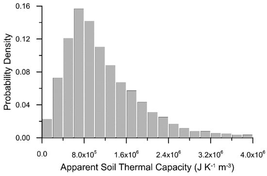
Figure 7.
Probability density of soil Apparent Thermal Capacity for TVGr.
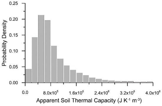
Figure 8.
Probability density of soil Apparent Thermal Capacity for TDCs.
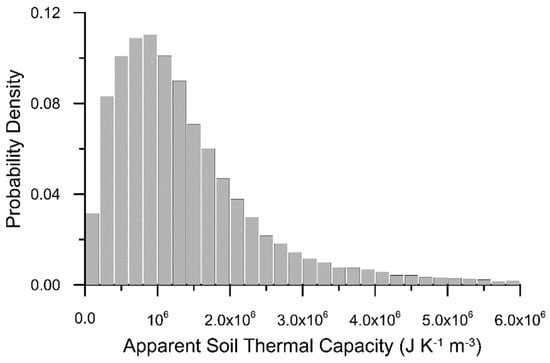
Figure 9.
Probability density of soil Apparent Thermal Capacity for CDGr.
3.2.2. Apparent Soil Thermal Conductivity
The one-dimensional theory of the heat thermal conductivity relates the heat flux G at depth z to the ground temperature vertical gradient:
where ks is the Apparent Thermal Conductivity. At the three non-urban locations, heat flux is measured at a depth of 5 cm and temperature at depths z1 = 2.5, z2 = 5 and z3 = 10 cm. From these measurements, values can be determined as described in Appendix B. Additionally, in this case, retrieved values are characterized by a high variability mostly attributable to the strong dependence of ks on soil water content. Table 4 reports ks mean, median and interquartile range for both rural and suburban stations. Comparing the mean and the median values, the difference between rural (TVGr and CDGr) and suburban (TDCs) stations is considerable. The thermal conductivity of rural soils is almost double that of the suburban, and the interquartile interval of the former is smaller than the analogous interval for the suburban station.
Table 4.
Soil Thermal Conductivity for the non-urban stations. Value for the soil layer between depths 0 and 5 cm of depth.
Figure 10, Figure 11 and Figure 12 show the probability density of the soil Apparent Thermal Conductivity obtained from the semi-hourly measurements at the three non-urban locations. Additionally, in this case, the distributions are not symmetrical and are characterized by a long tail towards the highest values representing sparse rain events of different intensities along the year.
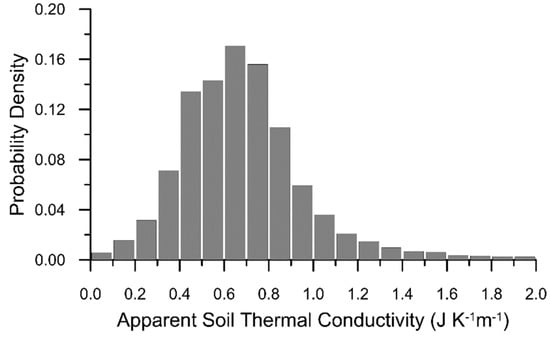
Figure 10.
Probability density of soil Apparent Thermal Conductivity at TVGr.
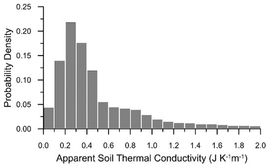
Figure 11.
Probability density of soil Apparent Thermal Conductivity at TDCs.
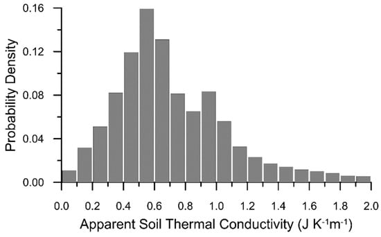
Figure 12.
Probability density of soil Apparent Thermal Conductivity at CDGr.
It is worth noting that the measures involved in the thermal conductivity estimation were located in the soil layer between the surface and the depth of 10 cm. Therefore, ks was relative to a portion of soil whose thermal characteristics could substantially differ from the soil portion below because of the normal agricultural operations activities.
3.2.3. Apparent Thermal Soil Diffusivity
The last differential relation describing the heat transmission into the ground, is supposed to be horizontally homogeneous in space and time, and is described through Fourier’s law:
where t is time, z is the depth and D the Apparent Thermal Diffusiveness, which depends on the water content of the soil. The method used to calculate the apparent thermal diffusivity from Equation (4) is given in Appendix C.
The estimated values of D show a daily and a seasonal variability that is linked to the water content in the soil. Additionally in this case, D was assumed as a stochastic variable whose statistical properties are summarized in Table 5. As expected, the D value for the rural station TVGr is slightly higher and compatible with the presence of sand soil [33], while in the other two stations the diffusivity value seems closer to the typical values of clay soil.
Table 5.
The apparent thermal diffusivity of soil D for the three non-urban stations. The reference value is for the soil layer between 0 and 5 cm of depth.
The variability of D is highlighted by the density probabilities reported in Figure 13, Figure 14 and Figure 15, that also in this case can be well represented by an asymmetric two-parameter distribution with the right tail linked to rain events of varying intensity distributed throughout the year.
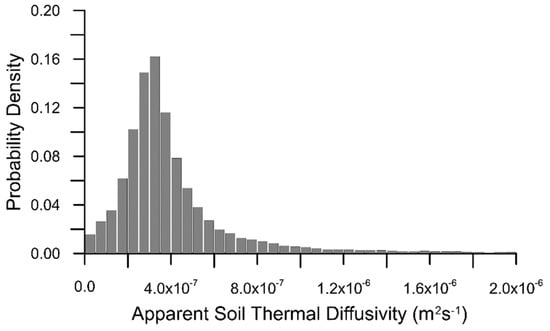
Figure 13.
Probability density of Apparent Thermal Soil Diffusivity at TVGr.
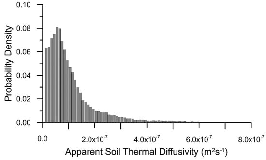
Figure 14.
Probability density of Apparent Thermal Soil Diffusivity at TDCs.
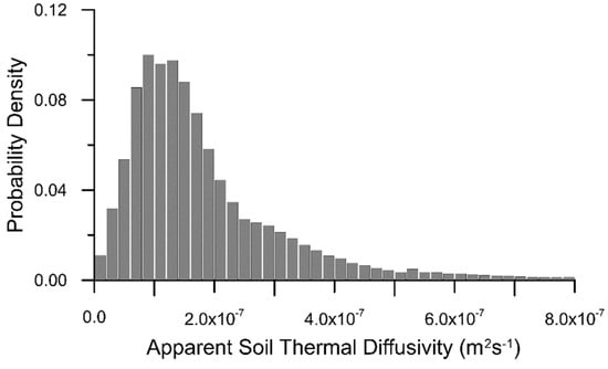
Figure 15.
Probability density of Apparent Thermal Soil Diffusivity at CDGr.
As previously mentioned, D and Ks retrievals refer to the soil layer between 0 and 10 cm, while Cs is estimated with respect to a deeper soil layer (5–50 cm). To verify whether the latter value differed from that calculated for the surface, the relationship between D, ks and Cs can be ascertained from the following relation [33]:
Table 6 reports the values of Cs determined in the layer 5–50 cm and 0–10 cm for the three non-urban sites. For the rural station TVGr the variation was minimal, implying that the soil was fairly homogeneous along the vertical and little disrupted by human activities. Conversely, the differences were much more marked for the rural station CGD and for the suburban station TDCs, where Cs value at the surface was about three times larger than that between 5 and 50 cm. Such a difference could be explained considering that TVGr soil is mainly wild, with only sporadic cuts of spontaneous vegetation, while CDGr and TDCs soil are subject to regular agricultural activity (Land use and soil maps of these areas can be found at [37]).
Table 6.
Apparent Thermal Capacity in the surface layer of soil and in the deep layer in the three non-urban locations.
3.3. Surface Roughness Parameters
The effect of surface irregularities on the vertical profiles of the average wind speed was parametrized with two different quantities, namely the zero-plane displacement height d and the roughness lengths z0, that account for the influence of large obstacles and surface roughness, respectively. To integrate and extend the analysis performed in [20], the following two subsections present d and z0 values for all the sites included in this study.
3.3.1. Zero-Plane Displacement Height
The parameter d represents the actual altitude from which the vertical profile of a variable starts because of the distortion of the air mass flux caused by significant geometric irregularity upwind to the site of measure. Morphological characteristics of the area around the three non-urban stations suggests that in these sites the parameter d can be neglected in all cases (i.e., d ≈ 0 regardless of wind direction), while the opposite situation holds for the urban site BNCu.
Following the method described in [38], under convective conditions the parameter d can be estimated from
where σw is the standard deviation of the vertical wind component and the coefficients a, b can be set at 1.07 and 4.29, respectively.
In principle, d could also be estimated in stable conditions, but in this case the acquired measurements turned out to be too noisy to perform a reliable analysis. In all probability, the intrinsic, instrumental noise added up to σw perturbations caused by gravity waves and submeso winds [39].
Taking into account convective (i.e., H0 > 0) conditions only, the selected half-hourly values acquired by the BNCu sonic anemometer installed at 30 m above the ground level were used to estimate d as a function of wind direction, clustering the results into sectors centered on the eight cardinal directions.
The results in terms of mean and median d values (Table 7) appeared to be strictly dependent on wind direction, reflecting the inhomogeneous distribution of buildings around the measurement site.
Table 7.
Zero-plane displacement height and roughness length z0 for the eight cardinal wind directions retrieved at BNCu stations.
3.3.2. Roughness Length
The relationship of the Monin–Obukhov Similarity Theory (MOST) which describes the vertical profile of the average wind speed U is:
where k is the constant of von Karman (equal to 0.4) and z is the altitude at which U refers. The similarity function for the vertical wind profile Ψm depends on the stability condition of the surface layer. Considering the stability parameter ζ defined as , when ζ < 0 (i.e., in convective situations) the similarity function is given by the following relationship:
where:
This relationship is accurate when |ζ| < 1.5, that is, when the turbulence is reasonably far from free convection. In stable situations, when ζ > 0, we have instead:
By inverting Equation (8), the roughness length z0 can be determined as:
Using the latter equation, the mean and the extremes of the interquartile range values of z0, as well as the number of available measurements were calculated for the four measurement sites as a function of the eight cardinal wind directions. Results are summarized in Table 7 (BNCu) and Table 8, Table 9 and Table 10 (TVGr, TDCs, CDGr). To avoid the inclusion of unreliable measures in the analysis, data with U < 1 m s−1 and < 0.05 m s−1 were discarded, and only convective or weekly stable conditions (−1.5 < ζ < 0.5) were considered. For the three non-urban stations d was set to zero, while for BNCU, values from the previous subsection were used.
Table 8.
Surface roughness z0 for TVGr.
Table 9.
Surface roughness z0 for TDCs.
Table 10.
Surface roughness z0 for CDGr.
The parameter z0 for the urban station varied little with the wind sector and was significantly higher than the typical values obtained for rural and suburban stations, reflecting the geometrical complexity that characterized a compact urban environment. As expected, CDGr, TDCs and TVGr sites showed a significant increase of z0 in the sectors where relevant geometric irregularities (upwind of the station) were present, highlighting the importance of wind direction in investigating and modelling complex environments.
4. Summary and Conclusions
Modelling complex phenomena such as pollutant dispersion or urban heat island requires a reliable estimation of surface properties that can be obtained only through long-term ABL observations. In this paper, a three-year dataset of micrometeorological measurements (albedo, surface properties, zero-displacement height and surface roughness) from four stations located in the city of Rome and its suburbs were analyzed and presented.
As expected, the integral albedo coefficient at the zenith for the urban station was found to be almost twice that for suburban and rural stations, with a value slightly higher than the maximum reported in literature, while its behavior as a function of solar elevation was in agreement with that previously published.
The zero-displacement height of the urban site located in Rome’s city center turned out to be strongly dependent on wind direction, as a consequence of the complex and inhomogeneous building distribution around the station, with values varying between 12.0 and 17.8 m. Conversely, the roughness length was almost independent of upwind direction however, it was significantly higher than the typical values calculated for the non-urban station (approximately 1.5 and 0.4 m, respectively), although the different measurements height of the stations prevented a direct comparison of the results. In addition, CDGr, TDCs and TVGr sites were characterized by a strong increase in z0 (up to a factor ≈ 12) in sectors where relevant terrain irregularities upwind of the station were recognizable by sight, reflecting the role of wind direction in modelling real surfaces.
For the first time, as far as we know, in situ data were used to estimate soil thermal properties over Rome’s area. Apparent thermal capacities and thermal conductivity at all the non-urban sites were in fair agreement with each other and typical of soil with relatively low water content, as expected for a relatively dry Mediterranean area like Rome. On the contrary, apparent thermal diffusivity appeared to be higher at TVGr than at the other two sites, reflecting the presence of different soil types, sand and clay soil at TVGr and CDGr/TDCs, respectively. In addition, the probability density of all the three parameters (regardless of the measurement site) showed a similar behavior, well-represented by an asymmetric two-parameter distribution such as log-normal, Weibull or gamma, with a long tail extending towards high values indicating the presence of heavy but sparse precipitation episodes, as expected in Mediterranean regions
Author Contributions
Data curation, R.S. and V.C.; Investigation, R.S., G.C. and I.P.; Methodology, R.S. and G.C.; Software, S.F.; Supervision, S.A.; Visualization, G.C.; Writing—original draft, A.C.; Writing—review & editing, G.C. All authors have read and agreed to the published version of the manuscript.
Funding
This research was funded by the EU LIFE project LIFE17 CCA/GR/000108—ASTI, implementation of a forecAsting System for urban heaT Island effect for the development of urban adaptation strategy.
Acknowledgments
The authors wish to thank ARPA Lazio and A. D. Di Giosa for providing the measurements used in this study.
Conflicts of Interest
The authors declare no conflict of interest.
Appendix A
Taking the depth z positive downwards, between the vertical heat flux G at z and the time variation of the mean temperature of the soil T at the same depth holds the relation expressing the principle of energy conservation given by Equation (2), where the Apparent Thermal Capacity is present. We can integrate this relation from 5 cm depth (z2), where G and T2 has been measured, down to 50 cm (z4), where T4 is available. The measurements of T4 obtained in the years at the non-urban stations have shown that its daily variation is negligible, and the annual variation is very small.
To estimate the apparent heat capacity of Cs every 30 min we have integrated Equation (2) from z4 to z2 assuming that the thermal capacity of the soil does not vary with the depth in this soil layer:
The time behavior of the temperature at z2, z3 and z4 allows a numerical estimate of the relative temporal derivatives. The numerical method used is discussed below. The Equation (A1) can therefore be rewritten as:
By approximating the integrals with the trapezoid method, the previous relationship becomes:
This relationship can be further simplified by taking into account that at depth z4 = 0.5 m the vertical heat flux is substantially zero and the temperature at the same depth shows practically negligible daily variations. This means that:
And
In this equation the only unknown variable is the thermal capacity of the soil that is:
The latter equation allows for the estimation of the soil thermal capacity, whose value may vary over time (for example, depending on the water content of the soil itself). Nevertheless, this equation presents a singularity when the denominator tends to zero and when both the numerator and the denominator tend to zero; in addition, Cs can be only positive. To overcome this problem, it has been assumed that the variation in time of Cs is relatively slow, so slow to be allowed to determine it as follows:
- first of all, Cs is calculated using Equation (A6) at a specific time-step ti;
- if it is negative, or positive but either higher than 107 or lower than 105 (J K−1 m−3), Cs at tj is assumed to be equal to that calculated at the previous time-step, tj − 1;
- in all other cases, Cs is calculated aswhere α is 0.9.
Appendix B
The Apparent Thermal Conductivity ks can be obtained by inverting Equation (3):
In this work, ks is estimated every 30 min with a finite difference approach using the heat flux G at z and the temperature T1, T2 e T3. As the three depths at which the temperature is measured are not equidistant, the numerical method suggested by [40] has to be used:
Using the latter, Equation (2.1) can be rewritten as:
It is worth noting that the use of this method presents some practical problems: during the daily evolution there are at least two instances during which the vertical gradient of temperature at different depths is cancelled. In correspondence of these time periods, the vertical flux of heat tends toward zero and it is not possible to estimate ks from the Equation (A10); in addition, noise contribution in the temperatures and the turbulent heat flux measurements, especially when the latter tends to zero, can lead to estimates of unrealistic negative values of ks, that need to be filtered out.
Appendix C
Inverting Equation (4), a relationship linking the Apparent Thermal Diffusivity to the temporal variation of the temperature and its second spatial derivative can be obtained:
The time series of mean temperature at depths z1, z2 and z3 allow for a direct estimation of D after having numerically approximated to the finite differences the partial derivatives present in Equation (3). At all time-steps different from the initial and final, the numerical approximations of the first and second partial derivative at depth z2 are calculated as follows [40]:
Values for which the second derivative cancels or both the derivatives tend to zero at the same time values.
References
- Schneider, A.; Friedl, M.A.; Potere, D. A new map of global urban extent from MODIS satellite data. Environ. Res. Lett. 2009, 4, 44003. [Google Scholar] [CrossRef]
- United Nations, Department of Economic and Social Affairs. Population Division 2015 World Urbanization Pospect: The 2014 Revision (ST/ESA/SER:A/266); United Nations: New York, NY, USA, 2015. [Google Scholar]
- Oke, T.; Cleugh, H. Urban heat storage derived as energy residuals. Bound. Layer Meteorol. 1987, 39, 233–245. [Google Scholar] [CrossRef]
- Ward, K.; Lauf, S.; Kleinschmit, B.; Endlicher, W. Heat waves and urban heat islands in Europe: A review of relevant drivers. Sci. Total Environ. 2016, 569, 527–539. [Google Scholar] [CrossRef] [PubMed]
- Silibello, C.; Bolignano, A.; Sozzi, R.; Gariazzo, C. Application of a chemical transport model and optimized data assimilation methods to improve air quality assessment. Air Qual. Atmos. Heal. 2014, 7, 283–296. [Google Scholar] [CrossRef]
- Martilli, A.; Clappier, A.; Rotach, M. An urban surface exchange parameterisation for mesoscale models. Bound. Layer Meteorol. 2002, 104, 261–304. [Google Scholar] [CrossRef]
- Kusaka, H.; Bornstein, R.; Ching, J.; Grimmond, C.; Grossman-Clarke, S.; Loridan, T.; Manning, K.; Martilli, A.; Miao, S.; et al. The integrated WRF/urban modelling system: Development, evaluation, and applications to urban environmental problems. Int. J. Climatol. 2011, 31, 273–288. [Google Scholar]
- Meng, X.; Evans, J.; McCabe, M. The influence of inter-annually varying albedo on regional climate and drouht. Clim. Dyn. 2013, 42. [Google Scholar] [CrossRef]
- Salleh, S.; Abd Latif, Z.; Chan, A.; Morris, K.; Ooi, M.C.G.; Naim, W. Weather Research Forecast (WRF) modification of land surface albedo simulations for urban near surface temperature. In Proceeding of the 2015 International Conference on Space Science and Communication (IconSpace), Kedah, Malaysia, 10–12 August 2015. [Google Scholar]
- Grimmond, C. Progress in measuring and observing the urban atmosphere. Theor. Appl. Climatol. 2006, 84, 3–22. [Google Scholar] [CrossRef]
- Eresmaa, N.; Karppinen, A.; Joffre, S.M.; Räsänen, J.; Talvitie, H. Mixing height determination by ceilometer. Atmos. Chem. Phys. 2006, 6, 1485–1493. [Google Scholar] [CrossRef]
- Mårtensson, E.M.; Nilsson, E.D.; Buzorius, G.; Johansson, C. Eddy covariance measurements and parameterisation of traffic related particle emissions in an urban environment. Atmos. Chem. Phys. 2006, 6, 769–785. [Google Scholar] [CrossRef]
- Lemonsu, A.; Leroux, A.; Bélair, S.; Trudel, S.; Mailhot, J. A General Methodology of Urban Cover Classification for Atmospheric Modeling; CRTI Scientific Report: Ottawa, OT, Canada, 2008. [Google Scholar]
- Vesala, T.; Järvi, L.; Launiainen, S.; Sogachev, A.; Rannik, Ü.; Mammarella, I.; Siivola, E.; Keronen, P.; Rinne, J.; Riikonen, A.; et al. Surface-atmosphere interactions over complex urban terrain in Helsinki, Finland. Tellus B 2008, 60, 188–199. [Google Scholar] [CrossRef]
- Järvi, J.; Hannuniemi, H.; Hussein, T.; Junninen, H.; Aalto, P.P.; Hillamo, R.; Mäkelä, T.; Keronen, P.; Siivola, E.; Vesala, T.; et al. The urban measurement station SMEAR III: Continuous monitoring of air pollution and surface–atmosphere interactions in Helsinki, Finland. Boreal Env. Res. 2009, 14, 86–109. [Google Scholar]
- Bergeron, O.; Strachan, I.B. Wintertime radiation and energy budget along an urbanization gradient in Montreal. Canada. Int. J. Climatol. 2012, 32, 137–152. [Google Scholar] [CrossRef]
- Nordbo, A.; Järvi, L.; Haapanala, S.; Moilanen, J.; Vesala, T. Intra-City Variation in Urban Morphology and Turbulence Structure in Helsinki, Finland. Bound. Layer Meteorol. 2013, 146, 469–496. [Google Scholar] [CrossRef]
- Baklanov, A.; Hänninen, O.; Slørdal, L.H.; Kukkonen, J.; Bjergene, N.; Fay, B.; Finardi, S.; Hoe, S.C.; Jantunen, M.; Karppinen, A.; et al. Integrated systems for forecasting urban meteorology, air pollution and population exposure. Atmos. Chem. Phys. 2007, 7, 855–874. [Google Scholar] [CrossRef]
- Bonacquisti, V.; Casale, G.R.; Palmieri, S.; Siani, A. A canopy layer model and its application to Rome. Sci. Total Environ. 2006, 364, 1–13. [Google Scholar] [CrossRef]
- Ciardini, V.; Caporaso, L.; Sozzi, R.; Petenko, I.; Bolignano, A.; Morelli, M.; Melas, D.; Argentini, S. Interconnections of the urban heat island with the spatial and temporal micrometeorological variability in Rome. Urban Clim. 2019, 29, 100493. [Google Scholar] [CrossRef]
- Colacino, M. Observations of a sea breeze event in the Rome area. Arch. Met. Geoph. Biokl. Ser. B 1982, 30, 127–139. [Google Scholar] [CrossRef]
- Aubinet, M.; Vesala, T.; Papale, D. Eddy Covariance: A Practical Guide to Measurement and Data Analysis; Springer: Netherlands, The Netherlands, 2012. [Google Scholar]
- Kaimal, J.C.; Finnigan, J.J. Atmospheric Boundary Layer Flows: Their Structure and Measurements; Oxford University Press: New York, NY, USA, 1994. [Google Scholar]
- Sozzi, R.; Valentini, M.; Georgiadis, T. Introduzione Alla Turbolenza Atmosferica: Concetti, Stime, Misure; Pitagora: Bologna, Italy, 2002. [Google Scholar]
- Finnigan, J.; Clement, R.; Malhi, Y.; Leuning, R.; Cleugh, H. A Re-evaluation of long-term flux measurement techniques Part I: Averaging and coordinate rotation. Bound. Layer Meteorol. 2003, 107, 1–48. [Google Scholar] [CrossRef]
- Finnigan, J. A Re-evaluation of long-term flux measurement techniques Part II: Coordinate systems. Bound. Layer Meteorol. 2004, 113, 1–41. [Google Scholar] [CrossRef]
- Grimmond, C.; Oke, T. Turbulent heat fluxes in urban areas: Observations and a local-scale urban meteorological parameterization scheme (LUMPS). J. Appl. Meteorol. 2002, 41, 792–810. [Google Scholar] [CrossRef]
- Robinson, G.D. Radiative Processes in Meteorology and Climatology; Paltridge, G.W., Platt, C.M.R., Eds.; Elsevier Scientific Publishing Company: Amsterdam, The Netherlands, 1976; p. 318. [Google Scholar]
- Offerle, B.; Grimmond, C.; Oke, T. Parameterization of net all-wave radiation for urban areas. J. Appl. Meteorol. 2003, 42, 1157–1173. [Google Scholar] [CrossRef]
- Pielke, R.A.S.R. Mesoscale Meteorological Modeling–2nd Edition; Academic Press: Cambridge, MA, USA, 2002. [Google Scholar]
- Philip, J. The theory of heat flux meters. J. Geophys. Res. 1961, 66, 571–579. [Google Scholar] [CrossRef]
- Sauer, T.; Horton, R. Soil heat flux. Am. Soc. Agron. 2005, 47, 131–154. [Google Scholar] [CrossRef]
- Garratt, J. The Atmospheric Boundary Layer; Cambridge University Press: Cambridge, UK, 1994. [Google Scholar]
- Schwerdtfeger, P. Physical Principles of Micro-Meteorological Measurements; Elsevier: New York, NY, USA, 1976. [Google Scholar]
- Gao, Z.; Fan, X.; Bian, L. An analytical solution to one-dimensional thermal conduction-convection in soil. Soil Sci. 2003, 168, 99–107. [Google Scholar] [CrossRef]
- Gao, Z. Determination of soil heat flux in a Tibetan short-grass prairie. Bound. Layer Meteorol. 2005, 114, 165–178. [Google Scholar] [CrossRef]
- Lazio Region Geo-Portal. Available online: https://geoportale.regione.lazio.it/geoportale/ (accessed on 28 January 2020).
- De Bruin, H.; Verhoef, A. A new method to determine the zero-plane displacement. Bound. Layer Meteorol. 1997, 82, 159–164. [Google Scholar] [CrossRef]
- Mahrt, L. Characteristics of submeso winds in the stable boundary layer. Bound. Layer Meteorol. 2009, 130, 1–14. [Google Scholar] [CrossRef]
- Ferziger, J.; Perić, M.; Street, R.L. Computational Methods for Fluid Dynamics; Springer: Heidelberg, Germany, 2002. [Google Scholar]


© 2020 by the authors. Licensee MDPI, Basel, Switzerland. This article is an open access article distributed under the terms and conditions of the Creative Commons Attribution (CC BY) license (http://creativecommons.org/licenses/by/4.0/).