Analysis of Air Pollution in Urban Areas with Airviro Dispersion Model—A Case Study in the City of Sheffield, United Kingdom

Abstract

Two air pollutants, oxides of nitrogen (NOx) and particulate matter (PM₁₀), are monitored and modelled employing Airviro air quality dispersion modelling system in Sheffield, United Kingdom. The aim is to determine the most significant emission sources and their spatial variability. NOx emissions (ton/year) from road traffic, point and area sources for the year 2017 were 5370, 6774, and 2425, whereas those of PM₁₀ (ton/year) were 345, 1449, and 281, respectively, which are part of the emission database. The results showed three hotspots of NOx, namely the Sheffield City Centre, Darnall and Tinsley Roundabout (M1 J34S). High PM₁₀ concentrations were shown mainly between Sheffield Forgemasters International (a heavy engineering steel company) and Meadowhall Shopping Centre. Several emission scenarios were tested, which showed that NOx concentrations were mainly controlled by road traffic, whereas PM₁₀ concentrations were controlled by point sources. Spatiotemporal variability and public exposure to air pollution were analysed. NOx concentration was greater than 52 µg/m³ in about 8 km² area, where more than 66 thousand people lived. Models validated by observations can be used to fill in spatiotemporal gaps in measured data. The approach used presents spatiotemporal situation awareness maps that could be used for decision making and improving the urban infrastructure.

1. Introduction

Air pollution has a significant negative impact on urban areas, especially in large megacities and roadside locations, where air pollution has become a growing issue for public health. Air pollution is causing numerous human health and environmental problems. Polluted air, especially with high levels of nitrogen dioxide (NO₂) and particulate matter with aerodynamic diameter of up to 10 µm (PM₁₀) and 2.5 µm (PM_2.5), is considered the most serious environmental risk to public health in urban areas in the UK [1]. Atmospheric pollutants were estimated to cause three million premature deaths in 2012 worldwide [2], whereas according to Landrigan [3], air pollution caused 6.4 million deaths worldwide in 2015. Air pollutants (e.g., NO₂ and PM₁₀) emitted by various emission sources are reported to cause heart disease, lung cancer and both chronic and acute respiratory diseases including asthma [2].

Air pollution models are numerical tools for describing the causal relationship of atmospheric pollutant concentrations with emissions, meteorology, deposition, chemical transformation and other factors like topography [4]. Modelling outputs can support Air Quality Monitoring Networks (AQMN) by improving spatial and temporal coverage in urban areas. Quantifying emission sources and predicting air pollutant concentrations using dispersion modelling approaches like Airviro, AERMOD or ADMS-Urban can help understand the main drivers of air pollution. Outputs of the dispersion model in the form of contour maps highlight spatial variability of air pollutant concentrations in the cities and provide a continuous maps that can be used to further fine-tune the air quality monitoring network.

Air quality modelling is carried out for several purposes, including air quality prediction/forecasting, analysing the dispersion of air pollutants in the atmosphere based on emissions and meteorological parameters, quantifying the impacts of air pollution (e.g., health impacts), modelling the impacts of various factors on air pollution, analysing the relationship between different pollutants, modelling pollution processes and transport, quantifying deposition and environmental fate of pollutants, running and testing emission scenarios, quantifying the emissions of air pollutants from various emission sources, determining long-term trends in air pollutant concentrations and producing high-resolution spatiotemporal maps of air pollution [5,6,7,8,9,10,11,12]. Dispersion models are also used for emergency planning of accidental chemical releases [13].

Air quality models can be divided into two main types, namely statistical and dispersion models. There is a wealth of statistical models, including time series (e.g., autoregressive moving average), regression (e.g., multiple linear regression), classification (e.g., logistic and discriminant analysis) and resampling methods (e.g., cross-validation and bootstraps) [14]. Dispersion modelling is further divided into Gaussian, Eulerian, Lagrangian, Computations Fluid Dynamics, Photochemical, Dense-gas, Aerosol Dynamic and Box models [15,16,17]. A number of techniques exist for modelling the dispersion of air pollutants, which vary in sophistication, but all include some sort of simplification of the real dispersion processes. Selecting a particular modelling approach depends on several factors such as the temporal and spatial scale of the model, resolution of the data available to run the model, the purpose of the modelling, skill of the modeller, time, and financial and computer resources available [16]. Dispersion modelling techniques for air quality are effective tools for determining downwind concentrations of air pollutants at a given time and space emitted by a known emission source, for example, an industrial plant or a nearby road. Dispersion models are mathematical representation of the atmospheric processes determining the rate at which pollutants are mixed with clean air. Results of dispersion models can be used to replace the need for air pollutant monitoring. However, the high cost of purchase and maintenance, high input demands and requirement of skilled staff limit their application.

In this paper, the Airviro version 4.01 dispersion modelling system [18] is employed to model the emissions of NOx and PM₁₀ in Sheffield, United Kingdom. The aim is to analyse different emission sources of air pollutants, investigate spatial variability of the pollutants, identify their main hotspots in Sheffield and assess the performance of Airviro model by comparing the modelled and observed concentrations in Sheffield. Furthermore, several emission scenarios will be tested which help identify the main drivers of air pollution in Sheffield. The rest of the paper is structured as follows: Methodology of this paper is presented in Section 2, where Section 2.1 presents the proposed framework, which includes the model for the air quality assessment of the Airviro dispersion. The air quality data and meteorological data are presented in Section 2.2. The assessment and validation of the proposed model is given in Section 2.3. Section 3 presents results and their analysis. The main outcomes of this work are summarised in Section 4.

2. Methodology

This paper presents a spatiotemporal analysis of the 2 air pollutants (PM₁₀ and NOx) sources, emissions and atmospheric concentrations in the city of Sheffield, United Kingdom. Air quality modelling and monitoring support each other in several ways. Air quality monitoring provides data only for points where the sensors are installed for the past and present time, whereas models provide better spatial coverage and, in addition to past and present, can predict air pollution concentrations for the future. Models validated by observations can be used to fill in spatiotemporal gaps in measured data. Figure 1 compares air quality monitoring and modelling and shows how they support each other.

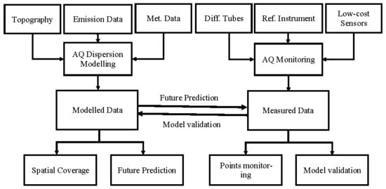
2.1. Dispersion Modelling System—Airviro

In this paper, Airviro version 4.01 was used, which is an air quality management system developed by Apertum [18,19]. Airviro is an integrated modelling system for managing emission inventories (Emission Data Base, EDB), modelling dispersion of pollutants and data handling. Airviro is a state-of-the-art dispersion model used by many researchers, consultants and local authorities globally for air quality modelling. Airviro has several modelling options [18,19]. In this study for urban scale modelling in Sheffield, a Gaussian model is used, which was introduced by Pasquill [20,21,22] and Briggs [23]. The Gaussian modelling technique is simple, computationally efficient and requires simple input data. Gaussian modelling is normally used for fast screening-type calculation of the pollutant dispersion in urban areas from point sources, line sources or area sources. Urban areas can be modelled as a sum of area sources (e.g., domestic and commercial emission), point sources (e.g., factory or power stations) and line sources (e.g., road traffic).

In this paper, two air pollutants, NOx and PM₁₀, are modelled using local topography, emissions and meteorological data to produce air quality maps of the estimated pollutants. In this paper, emissions of NOx and PM₁₀ from road traffic, point sources and area sources are modelled, and the estimated concentrations are compared with measured concentrations from several sensors. Dispersion models convert pollutant emissions to atmospheric concentrations in the form of contour maps and receptor points. This paper presents emission data, real case studies and the developed approaches for air pollution modelling and prediction.

In additional to annual levels, NOx and PM₁₀ concentrations are estimated for spring, summer, autumn and winter seasons and compared with measured concentrations at three receptors points (as discussed in Section 2.3).

2.2. Emission and Meteorological Data

Sheffield (53°23′ N, 1°28′ W) is a metropolitan borough and a vibrant city in South Yorkshire, United Kingdom. Historically known as the Steel City, Sheffield no longer has the smoking chimney stacks and has emerged as a green and modern cityscape in the proximity of the Peak District National Park. According to 2011 census, Sheffield City had a population of 552,700; however, since then, the population has grown and according to more recent estimates has reached about 700,000. Its elevation above sea level ranges from 29 m near Blackburn Meadows to 548 m near Margery Hill. Sheffield, like most of the United Kingdom, has a temperate climate with an average maximum temperature of 20.8 °C in June and July and an average minimum temperature of 1.6 °C in January and February.

Both spatial road traffic and points air pollutant emission sources are shown in Figure 2. In this paper, the Airviro EDB for Sheffield was used, which contains detailed information on the sources of emissions and allows for emission rates for various types of emission sources such as point sources, area sources or road sources to be calculated. This EDB has an updated 2017 road traffic data (emission factors, traffic counts, vehicle speed, and fleet composition), area sources (commercial and domestic emissions) and point (industrial) sources. The new emission factors (Emissions Factor Toolkit v8.0.1b) include nonexhaust particulate matter such as resuspension of dust particles. The EDB also takes account of spatiotemporal variability in emission rates. Emissions are calculated as a function of day type (e.g., weekday or weekend), hour of day and month of year. Temporal resolution of emissions is hourly, whereas the model outputs are presented in different time resolutions including hourly, seasonal or annual. For example, to calculate emissions for a road segment, the emission database uses some basic information including road name, road type (e.g., urban road, motorway etc.), vehicle speed, traffic counts, fleet composition, number of lanes, road length, slope and elevation. Likewise, to calculate emission from a point source, the emission database uses various information of the source such as name, location, coordinates, chimney characteristics (e.g., chimney height, outer and inner diameter of chimney, exhaust gas temperature and exhaust gas velocity), and characteristics of the emissions such as substance (e.g., NOx, PM₁₀, SO₂), amount of emissions and time variation of emissions. Full details on Airviro EDB are provided by Airviro User’s Reference [13]. Spatial resolution of area sources, which includes residential and commercial, is 1 km × 1 km. Point sources emissions are calculated individually. The Airviro EDB for 2017 shows that there were 268 point sources emitting 12,999 ton/year SO₂, 6774 ton/year NOx, 3077 ton/year CO and 1449 ton/year PM₁₀ in Sheffield and Rotherham. On the other hand, road sources emitted 5370 ton/year NOx and 345 ton/year PM₁₀. Emission data of some pollutants were missing in the database (

Table 1. Emission of various air pollutants (ton/year) in Sheffield and surrounding areas.

Pollutant	Point Sources	Road Sources	Area Sources	Total Emission
SO2	12999		1157	14156
NOx	6774	5370	2425	14569
NO2	122			122
CO	3077		2203	5280
PM10	1449	345	281	2075
PM2.5		224		224

). Several pollutants have demonstrated reduction in their emissions, e.g., SO₂ from road sources due to the effects of Directive 2005/33/EC of the European Parliament on the removal of sulphur from road traffic fuels. In addition, improvements in road vehicle fuels and technologies as a result of EU Directives on emission standards also resulted in reductions in CO from 65% (1990) to 16% (2017), in conjunction with reductions from industrial sources “due to the decline in the use of solid fuels in favour of gas and electricity, as well as a decline in the production of steel and non-ferrous metals” [24]. This study considers only two pollutants i.e., NOx and PM₁₀. Emissions of NOx and PM₁₀ are shown in Figure 3, demonstrating their spatial variability and highlighting hotspots in terms of pollutant emissions ((ton/year)/km²).

Hourly meteorological data including temperature, relative humidity and wind speed and direction (Figure 4) were measured at Woodburn Road weather mast in Sheffield, located at Sheffield Hallam University City Athletics Stadium. These were used for the simulation of hourly NOx and PM₁₀ concentrations, whereas for monthly, seasonal and annual scenarios, Airviro used a statistical approach for estimating such meteorological conditions. Before model runs, the meteorological data were used to determine the boundary layer scaling parameters—surface friction velocity and the Monin-Obukhov length. The wind fields were simulated using the diagnostic wind model available in Airviro, which considered the effects of topography, surface roughness and surface adiabatic heating/cooling [25]. Atmospheric conditions are classified into six (6) stability classes in the model: very stable, stable, neutral negative, neutral positive, unstable and very unstable [26].

2.3. Model Assessment

PM₁₀ and NOx concentrations (µg/m³) predicted by the Airviro model are presented in the form of contour maps. Predictions are also made for three receptor points, namely Devonshire Green, Sheffield Tinsley and Barnsley Road air quality monitoring stations, which are part of the UK Department for Environment, Food and Rural Affairs (DEFRA) Automatic Urban and Rural Network (AURN). Details of these sites are provided in

Table 2. Air quality monitoring sites (receptor points) where measured and modelled concentrations are compared.

Site Name	Site Type	Easting (X)	Northing (Y)	Pollutant Monitored	Monitoring Technique	Distance to Road (m)	Inlet Height (m)
Sheffield Tinsley (SHE)	Urban Industrial	440,215	390,598	NO2	Chemiluminescence	120 (M1)	3
Sheffield Devonshire Green (SHDG)	Urban Background	435,158	386,885	NO2, PM10, PM2.5, O3,	Chemiluminescence, TEOM, UV Absorption	20	3
Sheffield Barnsley Road (SHBR)	Urban Traffic	436,276	389,930	NO, NO2, NOx	Chemiluminescence	4.5	2

. Measured and modelled NOx and PM₁₀ concentrations are compared at these sites to assess the performance of the model. Comparisons are made for annual concentrations as well as for winter, spring, summer and autumn seasons. Furthermore, hourly predicted and observed concentrations are compared for the month of January, representing winter, and July, representing summer season 2017. Several statistical metrics are calculated to assess the performance of the model. The metrics used in this paper are the correlation coefficient (r), Root Mean Square Error (RMSE), Mean Bias (MB), Normalised Mean Bias (NMB), Mean Absolute Error (MAE), Normalised Mean Absolute Error (NMAE), Factor of two (FAC2) and Coefficient of Efficiency (COE).

The RMSE and Root Mean Square Deviation (RMSD) provide a good measure of the model error by calculating how close or far the predicted values are to the observed values. The RMSE measures the difference between the predicted and observed concentrations. The RMSE is a non-negative quantity, and ideally, we want it to have a zero value which means a perfect fit of the model having no error. MB is simply the average bias between the predicted and observed values. NMB is calculated by adding up the difference between the predicted and observed values (∑ (predi − obsi)) and normalising it by the sum of the observed values (∑obsi). NMB is reported as a percentage (%). NMB estimates average over or under prediction, and its value between +0.02 and -0.02 shows acceptable model performance. MAE provides a good indication of the mean absolute error and is in the same units as the quantities being considered. The MAE is normalized by dividing it by the observed value. The normalised value is known as NMAE. The correlation coefficient (r) characterises the strength of the linear relationship between two variables i.e., modelled and observed concentrations. The closer to one (±1) the value of r is, the better the similarity is. Generally, a value ranging from ±0.5 to ±0.99 indicates reasonably good performance of the model. FAC2 is the fraction of modelled values within a factor of 2 of the observed values. FAC2 should satisfy the condition that 0.5 ≤ predi/obsi ≤ 2. The ideal value for the FAC2 is 1 (100%). A highly efficient or perfect model should have COE value of 1. However, when analysing real data, a model has a COE value of less than 1. COE having a zero value (COE = 0) means the model prediction is not better than the mean of the observed value, which, in other words, means its prediction power is zero or it has no predictive advantage. These metrics are further described by [27,28].

3. Results and Discussion

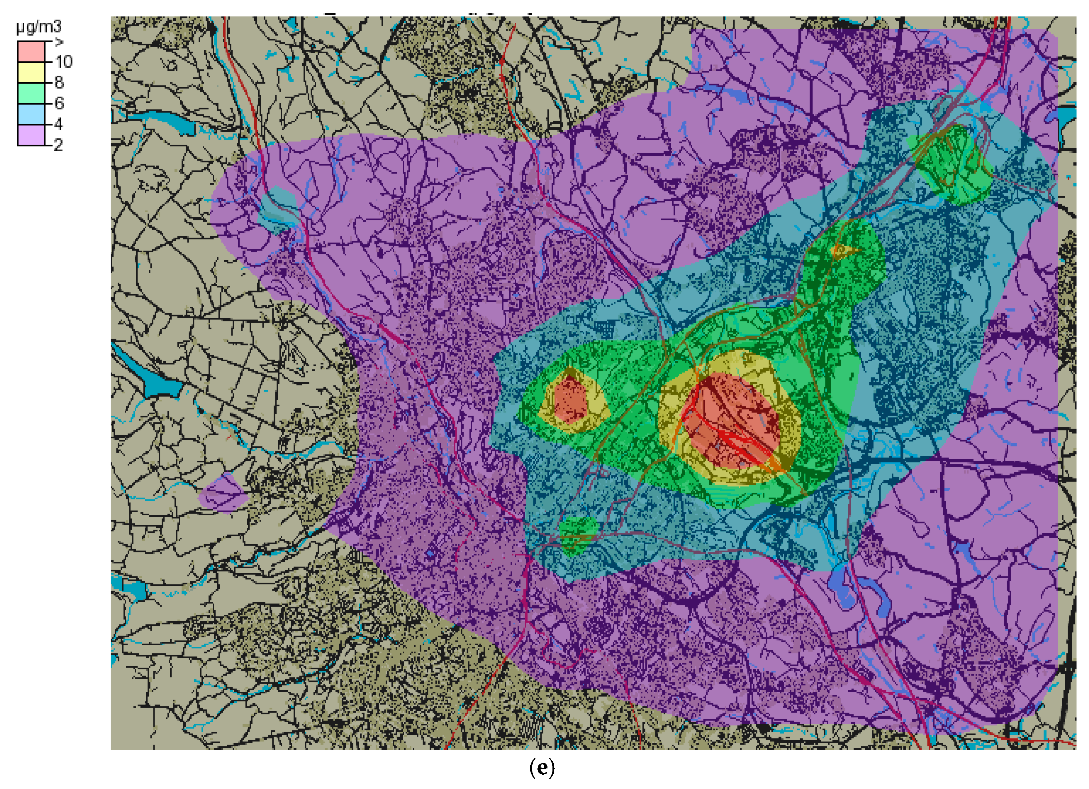
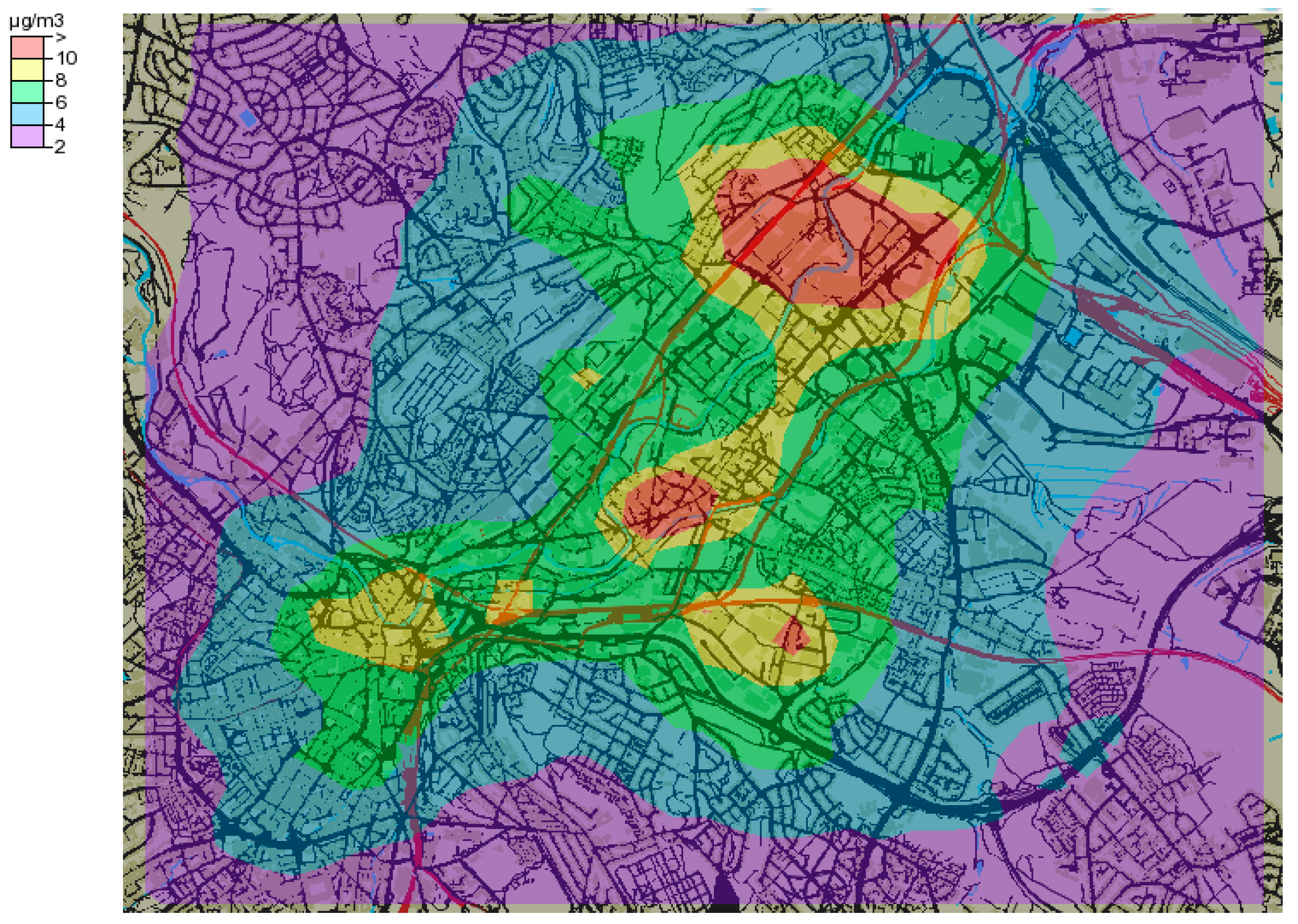
Employing the Airviro model, emissions (ton/year) of NOx and PM₁₀ are modelled to produce atmospheric concentrations (µg/m³) of these pollutants in the form of contour maps for the year 2017 in Sheffield. In Section 3.1, results of NOx, and in Section 3.2, results of PM₁₀ are presented and discussed.

3.1. NOx Maps

Figure 5 shows modelled annual average NOx concentrations (µg/m³) in the form of contour maps using traffic, points and area emission sources employing Gauss module for scenario 2017. Figure 5 shows three areas of high NOx concentrations in the city, namely Sheffield City Centre, Darnall and near Tinsley Roundabout (M1, J34S). High levels of NOx are also predicted on Sheffield Parkway (A630, A57) and between Meadowhall Shopping Centre and Sheffield Forgemasters International (a heavy engineering steel company). Sheffield City Centre probably experiences the highest levels of NOx, which is mainly due to the high level of road traffic, but various point and area sources also contribute. Pollution levels are highest in the busiest part of the city including St. Mary’s Gate, More Street, Eyre Street, Arundel Gate, Sheaf Street, Pond Street, Exchange Place and Castlegate. The train station, the bus station, the area of the Sheffield Hallam University and a busy shopping centre make this area very busy in terms of road traffic, exposing visitors, workers, students, commuters and residents to high levels of air pollution. Areas adjacent to the city centre also experience a considerable amount of air pollution. Generally, pollution levels gradually decrease with distance from the city centre. However, due to prevailing south-westerly winds and the locations of some industrial sources, there is a north-eastern trend in air pollution levels i.e., north-eastern region towards M1 experiences considerably high amount of air pollution (39–52 µg/m³) (Figure 5). In the north-eastern region, there are three hot spots where air pollution levels are higher (NOx levels > 65 µg/m³), namely Darnall, near Tinsley Roundabout on M1 J34S and between Sheffield Forgemaster International and Meadowhall Shopping Centre. The reasons for these hotspots are high traffic levels and some heavy steel industries. The north-eastern region experiences considerably more road traffic due to the Motorway (M1) and several major roads to and from Sheffield City Centre, Meadowhall and the M1.

Figure 6 shows the effect of various emission scenarios on atmospheric NOx concentrations in Sheffield, where Figure 6a represents emissions of road traffic, (b) represents HGV (Heavy Goods Vehicles) and LGV (Large Goods Vehicles), (c) represents cars, both petrol and diesel, (d) represents buses and (e) represents point sources in Sheffield. Here, HGV and LGV are European terms used for any vehicles or trucks with a gross weight of over 3500 kg. These different categories of emissions result in different spatial variability of NOx. The outputs of these scenarios show that the levels of NOx pollution are mostly controlled by road traffic. HGVs seem to emit a considerable amount of emissions in the city centre (Figure 6b), and their contribution is greater than that of the buses or cars. Scenario (6a), which represents all traffic modes, shows high pollution levels in the city centre and surrounding areas. Furthermore, it shows higher pollution levels along Sheffield Parkway leading to Motorway (M1) and along Penistone Road (A61). The other traffic scenarios show moderate levels of air pollution in the city centre and the adjacent areas. Figure 6e, which considers only point sources, represents a totally different spatial pattern of NOx concentrations. In this scenario, the hotspots in the city centre and surrounding areas have disappeared. Here, the two hotspots are in Tinsley (near J34SM1) and Attercliffe (near A6109). In Tinsley, there are about 15 point sources, whereas on both sides of A6109 (where the hotspot is shown), there are about 13 point sources, which are the most likely reasons for these two hotspots.

Atmospheric levels of NOx were estimated in various seasons of the year (Figure not shown for brevity), namely: (a) winter (November, December, January), (b) spring (February, March, April), (c) summer (May, June, July) and (d) autumn (August, September, October). Generally, atmospheric pollutant levels were higher in colder seasons due to (i) a greater combustion of fossil fuels—mainly diesel, petrol, gas and coal to a lesser extent and (ii) atmospheric stagnation and shallower atmospheric boundary-layer height, which discourage pollutant dispersion as compared to hotter seasons when the atmosphere is more turbulent and boundary layer height is wider. Mainly, there are four hotspots, which are Sheffield City Centre, Tinsley, near Forgemaster International and Darnall. The four seasons demonstrated slightly different patterns and levels of NOx. Relatively higher levels of NOx were predicted in winter and autumn, in which minimum, mean and maximum levels (µg/m³) were 4, 23, 87, and 2, 21, 91, respectively. Summer and spring showed relatively lower NOx levels, in which minimum, mean and maximum NOx levels (µg/m³) were 2, 16, 68 and 2, 19, 81, respectively.

3.2. PM₁₀ Maps

Figure 7 shows the results of modelled annual average PM₁₀ concentrations (µg/m³) in the form of contour maps using road traffic, point and area emission sources. Gauss module of Airviro for scenario 2017 was employed in this study. In contrast to NOx concentrations, the areas with elevated PM₁₀ concentrations are shown outside Sheffield City Centre. The highest PM₁₀ pollution levels were observed between Meadowhall Shopping Centre and Sheffield Forgemaster International. This hotspot seems to be due to the point sources (heavy steel and other companies) in this area. However, this is also a busy area in terms of road traffic, which must be contributing a significant amount of emissions. The second hotspot of PM₁₀ is shown in Attercliffe, which has six point sources emitting a significant amount of PM₁₀ and other pollutants. The third hotspot of PM₁₀ is shown in Sheffield Parkway, having three point sources. The fourth hotspot is the north-eastern corner of the city centre in the Wicker and West Bar near Derek Dooley Way. The model results demonstrate that PM₁₀ levels are affected more by the heavy industries rather than the road traffic, which is in contrast to NOx levels, which are more linked with road traffic. Figure 8, showing PM₁₀ concentrations estimated from point sources (a) and road traffic (b), provides further evidence that PM₁₀ levels in Sheffield are more affected by point sources. When only point sources were considered as inputs to the model, the minimum, mean and maximum PM₁₀ levels (µg/m³) were 0.24, 1.3, and 13.9, respectively, whereas when only road traffic was considered, these levels were 0.04, 0.56 and 2.5, respectively.

PM₁₀ concentrations (µg/m³) in various seasons of the year were also modelled and compared. PM₁₀ concentrations slightly varied and showed slightly different spatial patterns in various seasons. The minimum, mean, and maximum PM₁₀ concentrations (µg/m³) in winter, spring, summer, and autumn were: 1.0, 4.12, 15.4; 0.66, 3.75, 15.4; 0.47, 3.47, 15.5; and 0.75, 4.49, 19.0, respectively. Autumn showed relatively higher average (4.49 µg/m³) and maximum (19.0 µg/m³) PM₁₀ concentrations compared to other seasons.

3.3. Comparison of Predicted and Observed Concentrations

3.3.1. Comparison of Seasonal and Annual Data

Modelled and observed NOx and PM₁₀ concentrations cannot be compared in the form of contour maps because observed concentrations are not available in the form of contour maps. To make comparison with observed concentration, both NOx and PM₁₀ concentrations were predicted for three receptor points in Sheffield, namely Devonshire Green, Sheffield Tinsley and Barnsley Road air quality monitoring stations (AQMS). Details of these sites are provided in Table 2. NOx is monitored at all three sites; however, PM₁₀ is only monitored at Devonshire Green site, and therefore comparison of measured and modelled PM₁₀ is made only at Devonshire Green site.

Predicted and measured NOx and PM₁₀ concentrations are compared in

Table 3. Comparison of measured and predicted NOx and PM₁₀ concentrations (µg/m³) at Devonshire Green, Tinsley and Barnsley Road AQMS in various seasons in the year 2017.

Pollutant	Season 2017	Devonshire Green		Tinsley		Barnsley Rd
		Observed	Predicted	Observed	Predicted	Observed	Predicted
NOx	Winter	49.2	76.0	69.4	66.3	111.7	47.5
	Summer	23.3	58.3	30.5	50.6	63.6	31.2
	Autumn	27.3	79.6	41.4	73.3	73.8	47.2
	Spring	36.2	70.9	44.2	56.9	86.5	41.2
	Annual	33.9	65.5	46.3	56.4	83.7	38.8
PM10	Winter	15.8	6.98	Not monitored
	Summer	16.08	5.98
	Autumn	13.5	7.55
	Spring	19.0	7.19
	Annual	16.0	6.63

. Predicted NOx concentrations are higher than the observed concentrations at Devonshire Green and Tinsley and lower at the Barnsley Road AQMS. The encouraging fact is that the model has captured the seasonal trend in NOx concentrations, showing higher levels in winter and lower in summer. Devonshire Green and Tinsley are background sites, whereas Barnsley Road is an urban traffic (roadside) site; therefore, lower prediction of NOx as compared to observed concentrations at Barnsley Road site probably indicates that emission inventory for Barnsley Road has underestimated road traffic flow. Observed NOx levels are more than double the predicted concentrations at Barnsley Road site. However, there is a good positive correlation (r = +0.66) between observed and predicted concentrations. Correlation between observed and modelled NOx at Devonshire Green and Tinsley sites was slightly weaker (r = +0.46 at both sites). A comparison of predicted and observed PM₁₀ concentrations at Devonshire Green site showed lower predicted than observed PM₁₀ concentrations by a factor of more than two. Furthermore, there was a weak negative correlation (r = −0.18) between the observed and predicted PM₁₀ concentrations. However, the data are very limited: only five of each observed and predicted values were available for comparison; therefore, to make such comparison meaningful, long-term time series observed and predicted NOx and PM₁₀ concentrations are required, which are analysed in the next section.

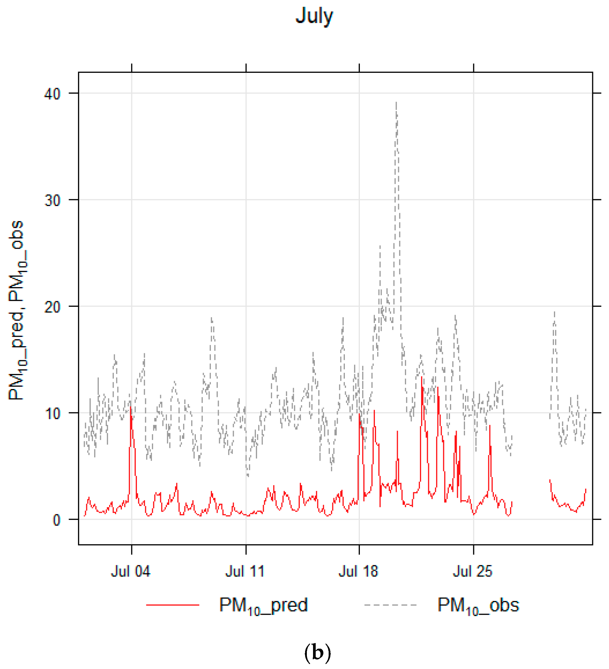
3.3.2. Comparison of Hourly Data

To compare hourly observed and predicted data, NOx concentrations were predicted for the months of January and July 2017 for Devonshire Green and Sheffield Tinsley. Comparison was not possible at Barnsley Road AQMS due to missing observed data for both January and July. PM₁₀ concentrations are monitored only at Devonshire Green monitoring station; therefore, comparison was not possible at the other two sites. To compare predicted and observed concentrations of NOx and PM₁₀, both a graphical approach and statistical metrics were used.

Predicted and monitored NOx concentrations (µg/m³) are compared for the months of January and July at Devonshire Green (DG) and Sheffield Tinsley (ST) AQMS. January represents winter, whereas July represents summer season of the year. The aim is to see how the model prediction varies in winter and summer seasons in comparison to observed data. Figure 9 shows the comparison of observed and predicted concentrations in January at Devonshire Green (upper-panel) and at Tinsley (lower-panel). At both Devonshire Green and Tinsley sites, the model is slightly under predicting NOx concentrations in January (Figure 9). Predicted mean and median concentrations at Devonshire Green in January were 40.29 and 28.20 and observed were 49.04 and 32.17, respectively, whereas at Tinsley predicted values were 51.21 and 27.40 and observed 63.25 and 42.75, respectively (

Table 4. Summary of the observed and predicted NOx concentrations (µg/m³) in January at Devonshire Green and Tinsley monitoring stations.

Metric	January
	Devonshire Green		Tinsley
	NOx_pred	NOx_obs	NOx_pred	NOx_obs
Minimum	0.83	2.73	1.30	3.24
1st Quartile	11.80	18.54	14.15	23.61
Median	28.20	32.17	27.40	42.75
Mean	40.29	49.04	51.21	63.25
3rd Quartile	46.85	61.23	58.05	78.78
Maximum	284.00	367.97	381.00	496.62

). Negative MB and NMB at both sites also show under-prediction (

Table 5. The value of various statistical metrics used for assessing the performance of the model for predicting NOx concentrations in the month of January 2017 at both Devonshire Green and Sheffield Tinsley.

Metric	Devonshire Green	Sheffield Tinsley
FAC2	0.65	0.52
MB	−8.67	−11.96
MAE	25.99	38.18
NMB	−0.18	−0.19
NMAE	0.53	0.60
RMSE	45.62	59.86
r	0.55	0.62
COE	0.22	0.12

). Metrics showing error of the model (e.g., MB, RMSE and MAE) are slightly greater at Tinsley, indicating larger difference between predicted and observed concentrations. However, the correlation coefficient value is also higher at Tinsley (0.62) than at DG (0.55), showing better linear association between predicted and observed concentrations. The model performance expressed by r (0.65) and FAC2 (0.52) is satisfactory in January at both receptor points.

Summary of predicted and observed NOx concentrations (µg/m³) for the month of July at both Devonshire Green and Tinsley is shown in

Table 6. Summary of the observed and predicted NOx concentrations (µg/m³) in July at Devonshire Green and Tinsley monitoring stations.

Metric	July
	Devonshire Green		Tinsley
	NOx_pred	NOx_obs	NOx_pred	NOx_obs
Minimum	3.95	2.10	5.42	4.56
1st Quartile	21.30	12.16	16.50	17.70
Median	32.10	16.62	26.10	27.48
Mean	35.78	19.73	38.71	32.00
3rd Quartile	40.45	23.47	46.05	40.30
Maximum	161.00	87.82	260.00	143.45

. In the month of July, predicted mean and median concentrations at Devonshire Green were 35.78 and 32.10, whereas observed concentrations were 19.73 and 16.62, respectively. At the Tinsley site, the predicted and observed mean and median concentrations were 38.71, 26.10, and 32.00, 27.48, respectively (Table 6). Minimum, mean, median and maximum values show over-prediction of the model in July at both sites. Various statistical metrics calculated for the month of July are shown in

Table 7. The value of various statistical metrics used for assessing the performance of Airviro model for predicting NOx concentrations in the month of July 2017 at both Devonshire Green and Sheffield Tinsley.

Metric	Devonshire Green	Sheffield Tinsley
FAC2	0.51	0.59
MB	16.05	6.78
MAE	19.40	23.58
NMB	0.81	0.21
NMAE	0.98	0.74
RMSE	28.15	36.36
r	0.32	0.34
COE	−1.24	−0.65

, where the values of MB and NMB also show that the model is over predicting NOx concentrations in July. Figure 10 graphically compares modelled and observed NOx concentrations, again showing slightly over-prediction of NOx concentrations.

Predicted and observed PM₁₀ concentrations (µg/m³) at Devonshire Green monitoring station are also compared in the month of January and July for the year 2017.

Table 8. Summary of the observed and predicted PM₁₀ concentrations (µg/m³) in the months of January and July 2017 at Devonshire Green monitoring stations.

Metric	January		July
	PM10_obs	PM10_pred	PM10_obs	PM10_pred
Minimum	1.50	0.15	4.00	0.24
1st Quartile	9.83	0.55	8.55	0.812
Median	15.20	1.57	10.35	1.46
Mean	17.77	3.17	11.12	2.05
3rd Quartile	22.80	3.17	12.69	2.38
Maximum	58.35	28.30	39.20	13.30

shows a summary of the predicted and observed PM₁₀ concentrations in both months. In January, the predicted mean and median concentrations were 3.17 and 1.57 and observed mean and median were 17.77 and 15.20, respectively. In July, predicted mean and median concentrations were 2.05 and 1.46 and observed mean and median concentrations were 11.12 and 10.35, respectively (Table 8), which clearly shows that the model under-predicts PM₁₀ concentrations in both January and July. This can also be observed in graphical presentations (Figure 11) and

Table 9. The value of various statistical metrics used for assessing the performance of the model for predicting PM₁₀ concentrations in the month of January and July 2017 at Devonshire Green monitoring station.

Metric	Devonshire Green
	January	July
FAC2	0.05	0.06
MB	−14.60	−9.07
MAE	14.84	9.07
NMB	−0.82	−0.82
NMAE	0.84	0.82
RMSE	17.59	9.90
r	0.46	0.40
COE	−0.74	−2.11

, which show significant difference in predicted and observed concentrations. FAC2 values are very low in the months of both January (0.05) and July (0.06). Furthermore, NMB value (−0.82) in both January and July shows under-prediction by the model. These values show that the model performance is not satisfactory for predicting PM₁₀ concentrations at Devonshire Green AQMS. RMSE values for the month of January and July were 17.59 and 9.90, respectively, whereas r values were 0.46 and 0.40 in January and July, respectively. Although the model under-predicts PM₁₀ concentrations in both months, it captures the trend; therefore, multiplying the modelled concentrations by a constant factor can bring the two time-series (observed and predicted concentrations) close together.

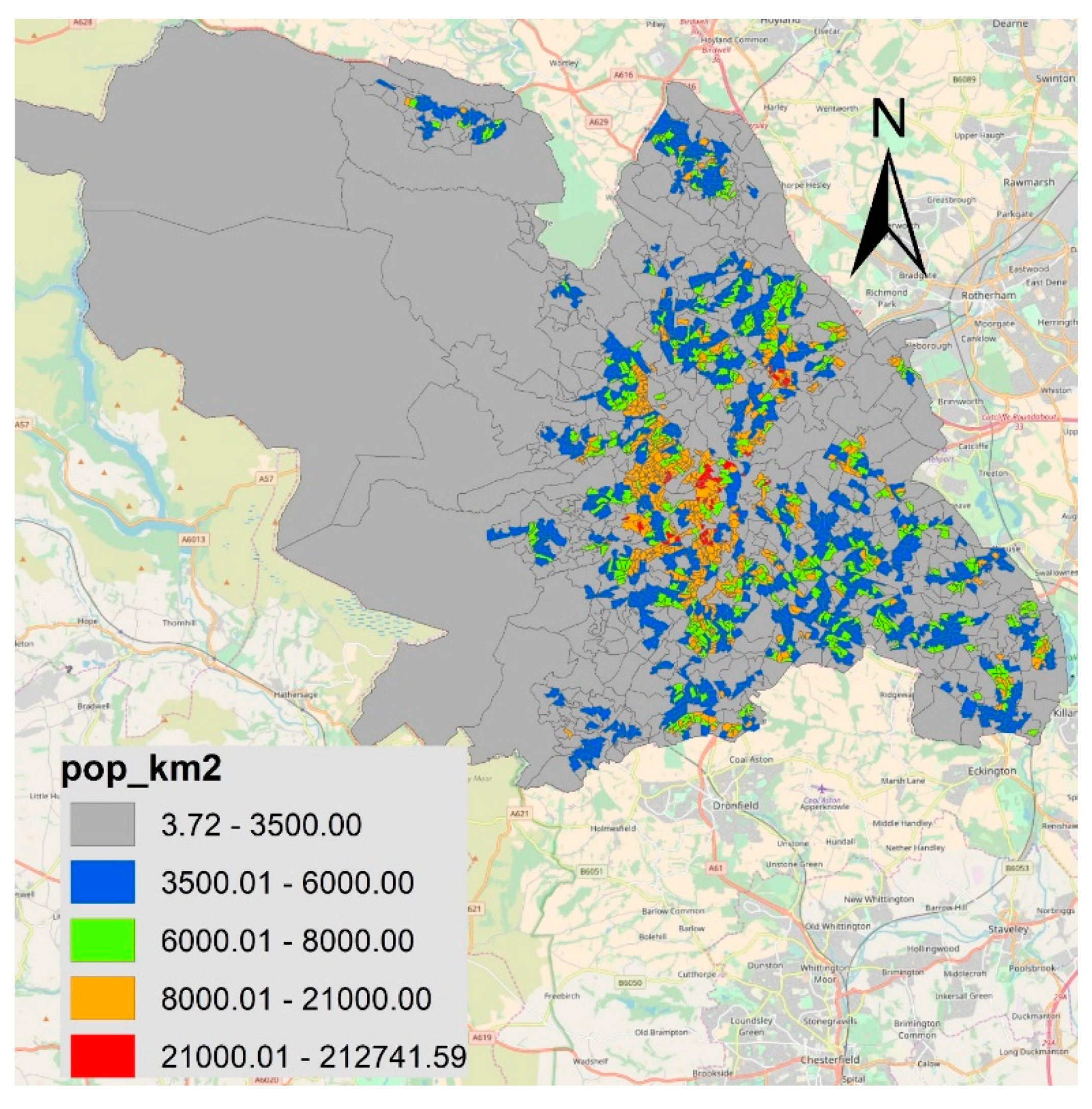
3.4. Population Exposure to Air Pollution

Modelled annual NOx concentrations (µg/m³) in the form of contour map are shown in Figure 5, which were obtained using emissions from road traffic, point and area sources employing the Gauss module of Airviro model. The main three hotspots of NOx in the city are shown, namely Sheffield City Centre, Darnall and near Tinsley Roundabout on M1 J34S. High levels of NOx are also predicted on Sheffield Parkway (A630, A57) and between Meadowhall Shopping Centre and Sheffield Forgemasters International. Sheffield City Centre is probably the most polluted part of the city, which is mainly due to the high level of road traffic.

In this section, Figure 5 is further analysed and the area of each colour representing a specific level of NOx concentrations is quantified. For this purpose, Figure 5 was exported to ArcGIS to calculate the area of each colour segment. Red colour, which shows NOx levels greater than 65 (µg/m³), had an area of 2.128 sq. km, whereas yellow colour, having NOx levels from 52 to 65 (µg/m³), had an area of 6.001 sq.km (

Table 10. Showing area (in km²) and estimated exposed population to air pollution in Sheffield (#: according to Figure 5 (showing NOx concentrations) and Figure 12 (showing population)).

Legends→	Red	Yellow	Green	Blue	Purple	Total
Area (sq.km)	2.128	6.001	20.533	36.269	43.308	108.239
Pop (# residents)	19218	47,517	81,201	160,797	143,023	451,756
NOx conc. (µg/m3)	>65	52–65	39–51	26–38	13–25	NA

). To calculate population exposure to NOx pollution, a population map (Figure 12) was used, which was provided by Sheffield City Council. As shown in Table 10, 19,218 people were estimated to live in the red area and 47,517 people were estimated to live in the yellow area. These are the areas mainly in and around the city centre of Sheffield. This provides evidence that most of the population exposure to high levels of air pollution in Sheffield is due to NOx pollution which is mainly emitted by road traffic (as discussed above).

Areas with high levels of PM₁₀ (Figure 7) are mostly outside the city centre, mainly in industrial areas, where population density is low. As discussed above, PM₁₀ pollution in Sheffield is mainly caused by point sources, which are mostly located outside the city residential area. Therefore, PM₁₀ pollution in Sheffield causes less population exposure compared to NOx pollution.

3.5. Further Discussion

Dispersion modelling systems are applied to predict (estimate) pollutant concentrations, which are reflective of emissions, meteorological and topographical data. Dispersion models in the UK are generally divided into screening, intermediate and advanced models [29]. Advanced models are utilised for assessment and review purposes at an urban scale using emissions from point, line and area sources. Among these, ADMS-Urban, AERMOD and Airviro modelling systems are frequently used throughout the world by local authorities, consultants and researchers.

There is always a degree of uncertainty in the model outputs, which is why the predicted concentrations are either lower or higher than the measured concentrations. These uncertainties are mainly due to two reasons [30]: (a) model inputs, including emission inventory, meteorological parameters, parameterisation of boundary layer and stability classes; (b) the model itself. Svensson [30] predicted NOx concentrations in Stockholm, Sweden using Airviro model and compared the results with measured concentrations, reporting that the model under-predicted NOx concentrations, especially in the winter season, which is in agreement with the current study. In this paper, PM₁₀ are significantly under-predicted, which seems to be mainly related to shortcomings in emission inventory. There are several possible sources of uncertainties in emission inventory that may cause the difference between modelled and measured PM₁₀ levels, including the following [31]: (a) Emission from diffuse sources, like emissions from coke ovens, metal processing and construction are difficult to be measured satisfactorily as their levels are variable in both time and space. (b) Combustion-related emissions are also subject to high uncertainty, especially in cases where PM emissions are very low and difficult to measure (e.g., from gas combustion or emissions from diesel vehicles with a particulate filter). (c) Emissions of PM from nonexhaust traffic sources, such as tyre and brake wear and road abrasion are particularly uncertain. (d) Coarse particles from resuspended soils and road dusts, are subject to considerable uncertainties. Furthermore, the emission inventory used in this study does not take into account secondary aerosols, which are formed in the atmosphere. The formation of secondary particles is dependent on the precursor’s emissions, e.g., SO₂ and NOx, that lead to the formation of secondary particles like nitrate (NO₃^-) and sulphate (SO₄^2-) and meteorological conditions like temperature and relative humidity. Secondary particles can contribute significantly into the observed concentrations of particles, especially fine particles (PM_2.5). Air Quality Expert Group (AQEG) [31] has shown that a significant amount of secondary particles made of nitrate and sulphate adding to the background concentrations is transferred from other large cities in the UK and Europe. Another possible reason for under-predicting PM₁₀ is the ignoring of small streets in emission inventory, which can directly contribute to the observed concentrations. According to AQEG, the estimated uncertainty in total UK emissions is estimated to be between –20% and +30%.

In a recent study, Dedele et al. [32] modelled NO₂ concentrations with Airviro in Kaunas, which is the second-largest city in Lithuania. They measured the levels of NO₂ using NO₂ diffusion tubes in five streets with different traffic and building characteristics for a two-week period in each season. Measured NO₂ concentration was higher in winter and autumn, and lower in spring and summer seasons, than the modelled concentrations. The difference between modelled and measured concentrations was greatest in winter, which was reported to be due to domestic heating in winter that was not accounted for in the model. Dedele et al. [32] reported that because the street canyon model did not take into account emissions from the other emission sources, it resulted in lower estimated values than measured values. Mukharjee et al. [26] also used Airviro to model the levels of NOx, SO₂ and CO in Singapore. They concluded that although road traffic contributed 24% NOx emissions in the city, the exposure caused was 40% due to the fact that the pollutants were emitted at the ground levels within the breathing zone. Leksomono et al. [29] also reported that industrial sources produced a relatively smaller contribution to ground-level NO₂ concentrations per unit of emission. This is because emissions from industrial sources are released at heights well above the ground and therefore subject to more dilution. According to the findings of Mukharjee et al. [26], the predicted and the measured hourly CO concentrations agreed to an accuracy of approximately 19% with R² value of 0.67. The model also captured the changes in the meteorological characteristics. The Airviro model over-predicted the measured NOx concentrations significantly, which was believed to be due to the constraint that the model did not take into account the photochemical transformation of NOx and ozone. Gidhagen et al. [33] employed Airviro model to assess the impact of residential wood combustion on exposure to PM_2.5 and its health impacts in three urbanised areas in Sweden. Gidhagen et al. [33] estimated that annual mortality due to modelled PM_2.5 concentrations from residential wood combustion was approximately four people (4 persons/year), corresponding roughly to 0.4% of the total number of deaths in the region. Leksmono et al. [29] have reported that distance of the site where meteorological data are collected from the area where pollution is to be modelled is important for assessing the levels of a pollutant, especially for modelling short-term concentrations.

The above discussion and the finding of this study indicate that dispersion-modelling systems are important tools for air quality management in urban areas; however, care should be taken to minimise the sources of error, which might include: (a) selection of appropriate model, (b) appropriateness of the emission inventory for the purpose, (c) availability of meteorological data and the distance of the meteorological monitoring site from the site of interest, (d) background contribution (both urban and regional), (e) photochemical transformation of pollutants and (f) complexity of the terrain.

4. Conclusions

Main aims of the study were (a) to determine the most significant emission sources of NOx and PM₁₀ in Sheffield; (b) to analyse spatiotemporal variability of NOx and PM₁₀ in Sheffield and surrounding areas, highlighting the hotspots of air pollution and discussing the main reasons; (c) to assess the performance of Airvrio air quality model for NOx and PM₁₀ prediction in different geographical locations in Sheffield during different times of the year.

In this paper, NOx and PM₁₀ pollutant emissions are modelled and their spatial distribution is analysed, employing the Airviro air quality dispersion modelling system. Air pollutant emissions from road traffic, point sources and area sources in Sheffield are modelled for the year 2017. Spatial variability of NOx and PM₁₀ concentrations is presented in the form of contour maps. Furthermore, NOx and PM₁₀ concentrations are predicted for three receptor points. Airviro outputs showed three locations with high NOx concentrations, namely Sheffield City Centre, Darnall and near Tinsley Roundabout on M1 J34S. High levels of NOx were also predicted on Sheffield Parkway and between Meadowhall Shopping Centre and Sheffield Forgemasters International. High PM₁₀ concentrations were estimated mainly between Sheffield Forgemasters and Meadowhall, near Sheffield Parkway and Attercliffe. Several emission scenarios were tested for both NOx and PM₁₀ which showed that high levels of NOx were mainly linked to road traffic, whereas those of PM₁₀ seemed to be linked with point sources. As expected, estimated levels of pollutants were higher in the colder season (e.g., winter) than in warmer season (e.g., summer). In the case of PM₁₀, predicted concentrations were significantly lower than the observed concentrations at the Devonshire Green monitoring station in both January and July; however, the model successfully captured temporal trends. Furthermore, modelled NOx concentrations showed better association with observed concentrations in terms of both pollutant levels and trends. Modelled NOx concentrations were also slightly lower in January and higher in July than measured concentrations. Spatial analysis showed that more people were exposed to NOx concentrations mostly emitted by road traffic in the city centre and surrounding areas than to PM₁₀ mostly emitted by point sources in Sheffield.

The main outcomes of this study can be summarized as follows: (1) NOx concentrations in Sheffield are mainly from road-traffic-related emission sources, whereas PM₁₀ concentrations are from point sources, e.g., various types of industries such as steel industry. (2) More people are exposed to NOx pollution mainly emitted by road traffics in the city centre. (3) There are three hotspots of NOx pollution in Sheffield, namely the Sheffield City Centre, Darnall and near the Tinsley Roundabout (M1 J34S), whereas the high PM₁₀ concentrations were shown mainly between Sheffield Forgemasters International and Meadowhall Shopping Centre. (4) Relatively higher average levels of NOx and PM₁₀ were predicted in winter and autumn than in summer and spring compared to measured concentrations. (5) NOx predictions by Airviro were lower in January and higher in July than measured NOx concentrations at both Devonshire Green and Sheffield Tinsley. However, the model under-predicted PM₁₀ concentrations in both January and July at Devonshire Green site. The difference between measured and predicted PM₁₀ concentrations was considerably greater compared to NOx. (6) In Sheffield, nearly 19,000 people live in areas with NOx levels greater than 65 µg/m³, and 48,000 people live in areas with NOx levels 52–65 µg/m³, which together are approximately 15% of the Sheffield population.

Models validated by observations can be used to fill in spatiotemporal gaps in measured air quality data. Furthermore, dispersion models are important tools for urban air quality management; however, steps should be taken to minimise potential errors in emission data, meteorological data and complexity of the terrain. Particulates generated from vehicle wear and tear, resuspension of dust particles and emission from natural sources require special attention to improve model performance. In addition, further work is required to quantify people’s exposure to air pollution in Sheffield using a dense network of static sensors and personal monitors. People can be exposed to air pollution in their houses (residents), workplaces and when commuting to and from work using various means of transports, e.g., buses, trains, trams, cars, bicycles or walking. How exposure levels vary using various transport modes needs to be quantified in Sheffield.

References

1. DEFRA. Improving Air Quality in the UK Tackling Nitrogen Dioxide in Our Towns and Cities, UK Overview Document. December 2015. Available online: https://www.gov.uk/government/uploads/system/uploads/attachment_data/file/486636/aq-plan-2015-overview-document.pdf (accessed on 9 June 2019).
2. WHO. Health Effects of Particulate Matter, Policy Implications for Countries in Eastern Europe, Caucasus and Central Asia; Publications of WHO Regional Office for Europe UN City; World Health Organization: Copenhagen, Denmark, 2013. [Google Scholar]
3. Landrigan, P.J. Air pollution and health. Lancet Public Health 2016, 2, 4–5. [Google Scholar] [CrossRef] [Green Version]
4. Daly, A.; Zannetti, P. Air Pollution Modeling—An Overview. Chapter 2 of Ambient Air Pollution; Zannetti, P., Al-Ajmi, D., Al-Rashied, S., Eds.; The Arab School for Science and Technology and The EnviroComp Institute: Half Moon Bay, CA, USA, 2007; Available online: http://home.iitk.ac.in/~anubha/Modeling.pdf (accessed on 18 August 2019).
5. Aldrin, M.; Haff, I.H. Generalised additive modelling of air pollution, traffic volume and meteorology. Atmos. Environ. 2005, 39, 2145–2155. [Google Scholar] [CrossRef]
6. Andersen, S.; Weatherhead, E.; Stevermer, A.; Austin, J.; Brühl, C.; Fleming, E.L.; De Grandpré, J.; Grewe, V.; Isaksen, I.; Pitari, G.; et al. Comparison of recent modeled and observed trends in total column ozone. J. Geophys. Res. Space Phys. 2006, 111, D02303. [Google Scholar] [CrossRef] [Green Version]
7. Arnold, S.R.; Chipperfield, M.P.; Blitz, M.A. A three-dimensional model study of the effect of new temperature-dependent quantum yields for acetone photolysis. J. Geophys. Res. Space Phys. 2005, 110, D22305. [Google Scholar] [CrossRef] [Green Version]
8. Baur, D.; Saisana, M.; Schulze, N. Modelling the effects of meteorological variables on ozone concentration—A quantile regression approach. Atmos. Environ. 2004, 38, 4689–4699. [Google Scholar] [CrossRef]
9. Berastegi, G.I.; Madariaga, I.; Elias, A.; Agirre, E.; Uria, J. Long term changes of O3 and traffic in Bilbao. Atmos. Environ. 2001, 35, 5581–5592. [Google Scholar] [CrossRef]
10. Brasseur, G.P.; Hauglustaine, D.; Walters, S.; Rasch, P.J.; Muller, J.-F.; Granier, C.; Tie, X.X. MOZART, a global chemical transport model for ozone and related chemical tracers: 1. Model description. J. Geophys. Res. Space Phys. 1998, 103, 28265–28289. [Google Scholar] [CrossRef]
11. Munir, S.; Chen, H.; Ropkins, K. Modelling the impact of road traffic on ground level ozone concentration using a quantile regression approach. Atmospheric Environ. 2012, 60, 283–291. [Google Scholar] [CrossRef]
12. Westmoreland, E.J.; Carslaw, N.; Carslaw, D.; Gillah, A.; Bates, E. Analysis of air quality within a street canyon using statistical and dispersion modelling techniques. Atmos. Environ. 2007, 41, 9195–9205. [Google Scholar] [CrossRef]
13. Wilkening, H.; Baraldi, D. CFD modelling of accidental hydrogen release from pipelines. Int. J. Hydrogen Energy 2007, 32, 2206–2215. [Google Scholar] [CrossRef]
14. James, G.; Witten, D.; Hastie, T.; Tibshirani, R. An Introduction to Statistical Learning: with Applications in R; Springer: New York, NY, USA, 2013. [Google Scholar] [CrossRef]
15. Salmond, J.A.; Clarke, A.G.; Tomlin, A.S. The Atmosphere; Harrison, R.M., Ed.; The Royal Society of Chemistry: London, UK, 2006; chapter 2; an introduction to pollution science; pp. 8–76. [Google Scholar]
16. El-Harbawi, M. Air quality modelling, simulation, and computational methods: A review. Environ. Rev. 2013, 21, 149–179. [Google Scholar] [CrossRef]
17. Modi, M.; Ramachandra, V.P.; Ahmed, L.S.K.; Hussain, Z. A review on theoretical air pollutants dispersion models. Int. J. Pharm. Chem. and Biol. Sci. 2013, 3, 1224–1230. [Google Scholar]
18. Airviro User’s Reference. Working with the Dispersion Module—How to Simulate the Dispersion of Pollutants; Swedish Meteorological and Hydrological Institute: Norrkoping, Sweden, 2013; Available online: https://www.airviro.com/airviro/extras/pdffiles/UserRef_Volume2_Dispersion_v3.23.pdf (accessed on 17 January 2019).
19. Airviro specification. Airviro Specification v4.00—Part I: Functions in Airviro. Apertum IT AB, Teknikringen 7- 583- 30. Linköping, Sweden. 2015. Available online: https://www.airviro.com/airviro/extras/pdffiles/Specification1_v4.00.pdf (accessed on 17 January 2019).
20. Pasquill, F. The estimation of the dispersion of windborne material. Meteorol. Mag. 1961, 90, 33–49. [Google Scholar]
21. Pasquill, F. Some observed properties of medium-scale diffusion in the atmosphere. Q. J. R. Meteorol. Soc. 1962, 88, 70–79. [Google Scholar] [CrossRef]
22. Pasquill, F. Atmospheric Diffusion, 2nd ed.; Horwood: Chichester, UK, 1974; ISBN 0853120153. [Google Scholar]
23. Briggs, G.A. A Plume Rise Model Compared with Observations. J. Air Pollut. Control. Assoc. 1965, 15, 433–438. [Google Scholar] [CrossRef]
24. National Atmospheric Emissions Inventory. Air Pollutant Inventories for England, Scotland, Wales, and Northern Ireland, 1990–2016. 2018. Available online: https://uk-air.defra.gov.uk/assets/documents/reports/empire/naei/annreport/annrep99/chap1_2.html (accessed on 8 July 2019).
25. Airviro User´s Reference. Working with the Emission Data Base (EDB): How to Construct a Dynamic Emission Database and Simulate Emission Scenarios, Version 4.00. 2018. Available online: https://www.airviro.com/airviro/extras/pdffiles/UserRef_Volume1_EDB_v4.00.pdf (accessed on 20 November 2019).
26. Mukherjee, P.; Viswanathan, S.; Choon, L.C. Modeling mobile source emissions in presence of stationary sources. J. Hazard. Mater. 2000, 76, 23–37. [Google Scholar] [CrossRef]
27. Carslaw, D. Defra Regional and Transboundary Model Evaluation Analysis—Phase 1, 15th ed.; King’s College London: London, UK, April 2011. Available online: https://uk-air.defra.gov.uk/assets/documents/reports/cat20/1105091514_RegionalFinal.pdf (accessed on 18 August 2019).
28. Sayegh, A.S. Comparing the Performance of Statistical Models for Predicting PM10 Concentrations. Aerosol Air Qual. Res. 2014, 14, 653–665. [Google Scholar] [CrossRef] [Green Version]
29. Leksmono, N.; Longhurst, J.; Ling, K.; Chatterton, T.; Fisher, B.; Irwin, J. Assessment of the relationship between industrial and traffic sources contributing to air quality objective exceedences: A theoretical modelling exercise. Environ. Model. Softw. 2006, 21, 494–500. [Google Scholar] [CrossRef]
30. Svensson, N. Evaluation of Atmospheric Dispersion Models: Comparison with Measurements in Stockholm. Master degree project in meteorology, Stockholm University, Stockholm, Sweden, 2013. [Google Scholar]
31. AQEG. Fine Particulate Matter (PM2.5) in the UK. Available online: https://uk-air.defra.gov.uk/assets/documents/reports/cat11/1212141150_AQEG_Fine_Particulate_Matter_in_the_UK.pdf (accessed on 21 November 2019).
32. Dėdelė, A.; Miškinytė, A.; Česnakaitė, I. Comparison of Measured and Modelled Traffic-Related Air Pollution in Urban Street Canyons. Pol. J. Environ. Stud. 2019, 28, 3115–3123. [Google Scholar] [CrossRef]
33. Gidhagen, L.; Bennet, C.; Segersson, D.; Omstedt, D. Exposure Modeling of Traffic and Wood Combustion Emissions in Northern Sweden—Application of the Airviro Air Quality Management System. IFIP Adv. Inf. Commun. Technol. 2015, 448, 242–251. [Google Scholar]
Figure 1. Schematic diagram comparing air quality modelling and monitoring and how they support each other.
Atmosphere 11 00285 g001
Figure 2. Emission sources in Sheffield and surrounding areas including Rotherham for the year 2017: (a) point sources, (b) road network or line sources.
Atmosphere 11 00285 g002
Figure 3. Emissions’ strength ((ton/year)/km2) in Sheffield and surrounding areas including Rotherham for the year 2017 from all emission sources: (a) NOx emissions, (b) PM10 emissions.
Atmosphere 11 00285 g003
Figure 4. Breuer frequency distribution (wind rose) for year 2017 weather data used in the Airviro model.
Atmosphere 11 00285 g004
Figure 5. Estimated annual mean NOx concentrations (µg/m3) using all emission sources in Sheffield for year 2017.
Atmosphere 11 00285 g005
Figure 6. Estimated mean annual NOx concentrations (µg/m3) using emissions from road traffic (a), HGV and LGV (b), cars both petrol and diesel (c), buses (d) and points sources (e) in Sheffield for the year 2017.
Atmosphere 11 00285 g006aAtmosphere 11 00285 g006bAtmosphere 11 00285 g006c
Figure 7. Estimated annual mean PM10 concentrations (µg/m3) using all emission sources in Sheffield City Centre for the year 2017.
Atmosphere 11 00285 g007
Figure 8. Estimated PM10 concentrations (µg/m3) from point sources (a) and road sources (b) in Sheffield.
Atmosphere 11 00285 g008
Figure 9. Comparison of predicted (pred) and observed (obs) NOx at both Devonshire Green (dg) and Sheffield Tinsley (tins) for the month of January 2017.
Atmosphere 11 00285 g009aAtmosphere 11 00285 g009b
Figure 10. Comparison of modelled and monitored NOx at both Devonshire Green (dg) and Sheffield Tinsley (tins) for the month of July 2017.
Atmosphere 11 00285 g010
Figure 11. A comparison of measured and predicted PM10 concentrations (µg/m3) at Devonshire Green Sheffield in the month of January (a) and July 2017 (b).
Atmosphere 11 00285 g011aAtmosphere 11 00285 g011b
Figure 12. Population density (residents/km2) map of Sheffield, 2016.
Atmosphere 11 00285 g012