Geoengineering: Impact of Marine Cloud Brightening Control on the Extreme Temperature Change over East Asia

Abstract

We investigated the effect of artificial marine cloud brightening on extreme temperatures over East Asia. We used simulation data from five global climate models which have conducted the GeoMIP G4cdnc experiment. G4cdnc was designed to simulate an increase in the cloud droplet number concentration of the global marine lower clouds by 50% under the greenhouse gas forcing of the RCP4.5 scenario. G4cdnc decreased the net radiative forcing in the top of the atmosphere more over the ocean, alleviating the rise in mean temperature under RCP4.5 forcing. For extreme temperatures, G4cdnc reduced both the monthly minimum of daily minimum temperature (TNn) and monthly maximum of daily maximum temperature (TXx). The response of TNn was higher than that of TXx, especially in the winter, over the Sea of Okhotsk and the interior of the continent. This spatial heterogeneity and seasonality of the response were associated with sea ice–albedo and snow–albedo feedbacks. We also calculated the efficacy of warming mitigation as a measure of the relative effect of geoengineering. The efficacy for TXx was higher than that for TNn, opposite to the absolute effect. After the termination of geoengineering, both TNn and TXx tended to rapidly revert to their trend under the RCP4.5 forcing.

1. Introduction

Since the industrial revolution, atmospheric concentrations of greenhouse gases (GHGs) have risen owing to anthropogenic activities. In particular, the rise in concentration of carbon dioxide has accelerated, recently exceeding 400 ppm. This has resulted in global warming, which is causing significant increases in the duration, frequency, and/or intensity of various types of extreme weather and climate events over East Asia and across the world. Many efforts have been devoted to solving the problems caused by global warming. For example, the Paris Agreement was signed by the United Nations Framework Convention on Climate Change (UNFCCC) in 2015 and aimed at limiting the increase in the global mean temperature to well below 2 °C above pre-industrial levels, and pursuing efforts to limit the increase to 1.5 °C. Each nation participating in the Agreement thus set an individual goal for the reduction of greenhouse gases and consented to meet it. However, it has been suggested that the Agreement is not sufficient to alleviate the damage caused by climate change [1]. Therefore, the geoengineering field is emerging; it is aimed at mitigating the adverse effects of global warming and has received significant attention. Geoengineering includes a broad set of methods and technologies aimed at purposely altering the climate system to alleviate the impacts of climate change, although concerns have been expressed regarding its implementation [2,3,4]. Geoengineering methods can be divided into two categories: carbon dioxide removal (CDR) and solar radiation management (SRM). The SRM method can be implemented in a variety of ways; the following has been suggested: using space mirrors in orbit [5], injecting aerosols into the stratosphere [6,7], and marine cloud brightening [8]. Marine cloud brightening is the focus of this study as it has received less attention.

Since the introduction of SRM, many studies investigating the effect of SRM on temperature and precipitation through climate models have been conducted [9,10,11]. However, it is difficult to compare these studies owing to different experimental designs and the dependency of using specific climate models. To solve these problems, the Geoengineering Model Intercomparison Project (GeoMIP) was initiated, along with an experimental design of each SRM method [12]. GeoMIP has been progressed over Phase 1, Phase 2, and Phase 6. Among those phases, GeoMIP Phase 2 deals with marine cloud brightening with three experimental designs according to the degree of complexity: the G1ocean-albedo experiment simulates an increase in the global ocean albedo; the G4cdnc experiment simulates an increase in the cloud droplet number concentration (CDNC) in the global lower marine clouds; the G4sea-salt experiment injects sea salt particles into the tropical oceans [13]. This study focused on the G4cdnc experiment, which is based on the indirect effect of an increasing cloud albedo by adjusting the CDNC [14]. Various climate models were used in the simulation in this study owing to the simplistic design, which yields a more complete multi-model ensemble [15].

Global warming has increased the global mean temperature and frequency of extreme events [16]. Because increased extreme temperature events are more easily recognized by society and have more immediate detrimental consequences than changes in the mean temperature, studying the changes in temperature extremes is necessary. Changes in extreme temperatures are characterized by a significant amount of regional variations, and previous reports reveal that extreme temperatures have been increased more over mid to high-latitude regions, including East Asia [17,18,19,20,21,22,23]. However, a response of extreme temperature over East Asia under geoengineering has not been studied yet.

Therefore, in this study, the effect of marine cloud brightening over East Asia is investigated using the output of the model which have conducted the GeoMIP Phase 2 G4cdnc experiment, focusing on the changes in extreme temperatures. In Section 2, the data and methods used for the analysis are described. With a brief examination of changes in radiative flux and mean temperature, Section 3 details the response of extreme temperature over East Asia via the G4cdnc experiment. Finally, Section 4 summarizes the results and conclusions of this study.

2. Data and Methods

2.1. Data

In this study, we used simulation data of the GeoMIP Phase 2 G4cdnc experiment from five global climate models (GCMs) out of nine models publicly available online (

Table 1. Description of earth system models of the GeoMIP G4cdnc experiment used in this study.

Model	Institution	No. of Grid Cells (lon × lat)	Termination Effect Experiment	Reference
BNU-ESM	Beijing Normal University, China	128 × 64	Yes	[25]
CanESM2	Canadian Centre for Climate Modeling and Analysis, Canada	128 × 64	Yes	[26]
CSIRO-Mk3L-1-2	University of New South Wales, Australia	64 × 56	Yes	[27]
HadGEM2-ES	Met Office Hadley Centre, UK	192 × 145	Yes	[28]
MIROC-ESM	Japan Agency for Marine-Earth Science and Technology, Japan	128 × 64	No	[29]

). The G4cdnc experiment simulates an increase in the CDNC in marine low clouds for a 50-year period, from 2020 to 2069. After the year 2070, the increase in CDNC is terminated, and it is restored to the level before the implementation of G4cdnc. The experiment continued until 2090 to evaluate the effect of terminating the CDNC [13]. The G4cdnc experiment is simulated under the Coupled Model Intercomparison Project 5 (CMIP5) RCP4.5 scenario, a medium stabilization scenario among the four representative concentration pathways (RCPs), assuming emissions of GHGs resulting in an atmospheric CO₂ concentration of 540 ppm by 2100 [24].

To investigate the effects of the G4cdnc experiment for extreme climate events, we focused our analyses on monthly minimum and maximum extreme temperatures instead of annual values. Analysis using monthly extremes enables us to consider monthly variations (i.e., seasonality) and identify extremes more precisely. To this end, we calculated TNn, a monthly minimum of daily minimum temperatures, and TXx, a monthly maximum of daily maximum temperatures, as defined by the Expert Team of Climate Change Detection and Indices (ETCCDI) [30]. These extreme indices have been frequently used in previous research, both for observed weather [31] and model simulations (Orlowsky and Seneviratne with Curry et al. for GeoMIP Phase 1 G1 experiment, Aswathy et al. for G3 and Ji et al. for G1 and G4) [32,33,34,35].

In the GeoMIP G4cdnc experiment under the RCP4.5 scenario, four models simulated daily minimum (TASmin) and daily maximum (TASmax) temperatures with regard to extreme climatic events. The BNU-ESM model, however, did not simulate these variables. Moreover, the MIROC-ESM model simulated only the increase in CDNC, without the termination of the experiment. Therefore, we excluded the BNU-ESM model from the analysis of extreme temperatures and the MIROC-ESM model from the analysis after the termination of the experiment.

As the spatial resolutions of simulation data differ between the models, as indicated in Table 1, all outputs by G4cdnc and RCP4.5 models were re-gridded to 144 × 73 (2.5° longitude × 2.5° latitude) for the convenience of comparison and calculation. The interpolation was carried out using the Climate Data Operators (CDO) package, in which we chose a first-order conservative remapping algorithm [36]. To analyze the changes over East Asia, we selected an analysis domain of 20–60° N, 90–160° E.

2.2. Methods

To investigate the effect of the GeoMIP G4cdnc geoengineering experiment over East Asia, we selected three periods for analysis: base period: 2006–2019, progress period: 2060–2069, and termination period: 2081–2090. For the base period, we used RCP4.5 data, and for the progress and termination periods, both G4cdnc and RCP4.5 data were used. Although many studies for geoengineering have adopted a 40-year period for analysis [33,35,37], we adopted only the last 10 years from the progress and termination periods to sufficiently consider the saturated conditions of forcing.

To obtain better insights into the changes in extreme temperature, we checked the changes in mean temperature through the calculation of probability density functions (PDFs) of monthly temperatures. To create PDFs of monthly temperature, the method reported by Curry et al. and Ji et al. was employed [33,35]. At every grid point in each model, we first calculated the standardized monthly anomalies of monthly mean surface temperatures in the base period under RCP4.5; i.e., ${\tau }_m^{Base}=\left(T_m^{Base}-{\overline{T}}_m^{Base}\right)/{\sigma }_{T_m}^{Base}$, where the overline denotes the monthly mean during the last 10 years of the progress period and ${\sigma }_{T_m}^{Base}$ the interannual monthly standard deviation for each month m. Next, we computed the monthly anomalies in perturbed experiments relative to the mean and standard deviation under RCP4.5 in the base period, i.e., ${\tau }_m^{Exp}=\left(T_m^{Exp}-{\overline{T}}_m^{Base}\right)/{\sigma }_{T_m}^{Base}$. For the progress period, PDFs were calculated for each individual model shown in Table 1 and for the multi-model ensemble; equal weights were used for each model. Then, we conducted a two-sample non-parametric Kolmogorov–Smirnov test to determine if the distribution under G4cdnc differs significantly from that under the RCP4.5 scenario in the progress period [38].

For extreme temperatures, we took the results of the difference between G4cdnc and its base experiment of RCP4.5 to investigate the effect of marine cloud brightening over East Asia. The change in the extreme temperature was investigated in terms of both temporal and spatial aspects, which were displayed using a timeseries and a field of the difference, respectively. For temporal changes, the mean of the difference deduced from the multi-model ensemble over both the progress and termination periods are printed on the upper right of the time series. Extreme temperatures in summer (JJA) and winter (DJF) were calculated to examine the effects of seasonality.

In the perspectives of establishing policies on local climate change, relative effects of geoengineering to warming magnitude under RCP4.5 may be more important than absolute effects. To consider this relative effect of G4cdnc, we adopted a simple quantitative metric, efficacy used in [33,39]. To do so, we first computed the root mean square (RMS) differences between experiments at each grid point as the following equation:

$$RM{S}_{Exp-Base}\left(X\right)=\sqrt{\frac{\sum \left(X_{Exp}-X_{Base}\right)2dA}{\sum dA}}$$

(1)

where X is the extreme index of interest, Exp the perturbed experiment (G4cdnc or RCP4.5 in progress period), Base the base experiment (RCP4.5 in base period), and ∑ a sum over the grid cells (dA) of a specified area A. Then, we calculated the efficacy e(X) of G4cdnc defined by the following equation:

$$e\left(X\right)\equiv 1-\frac{RM{S}_{G4cdnc-Base}\left(X\right)}{RM{S}_{RCP4.5-Base}\left(X\right)}$$

(2)

In the case of e(X) → 1, the temperature under G4cdnc approaches the temperature in the RCP4.5 base period so that the G4cdnc experiment is the most effective in offsetting the warming under the RCP4.5 scenario. On the other hand, e(X) → 0 indicates that the G4cdnd experiment has little effect in reducing the warming. Values of e(X) can be negative if RMS differences for G4cdnc exceed those for RCP4.5. Efficacy was calculated for mean temperatures (TAS, TASmax, and TASmin) as well as for the two extreme temperature indices (TNn and TXx) to check if there are significant differences between relative effects on extreme temperatures and mean temperatures. We also analyzed the efficacy not only for the progress period but also for the period after the termination of geoengineering in order to investigate how long the relative effects can last.

3. Results

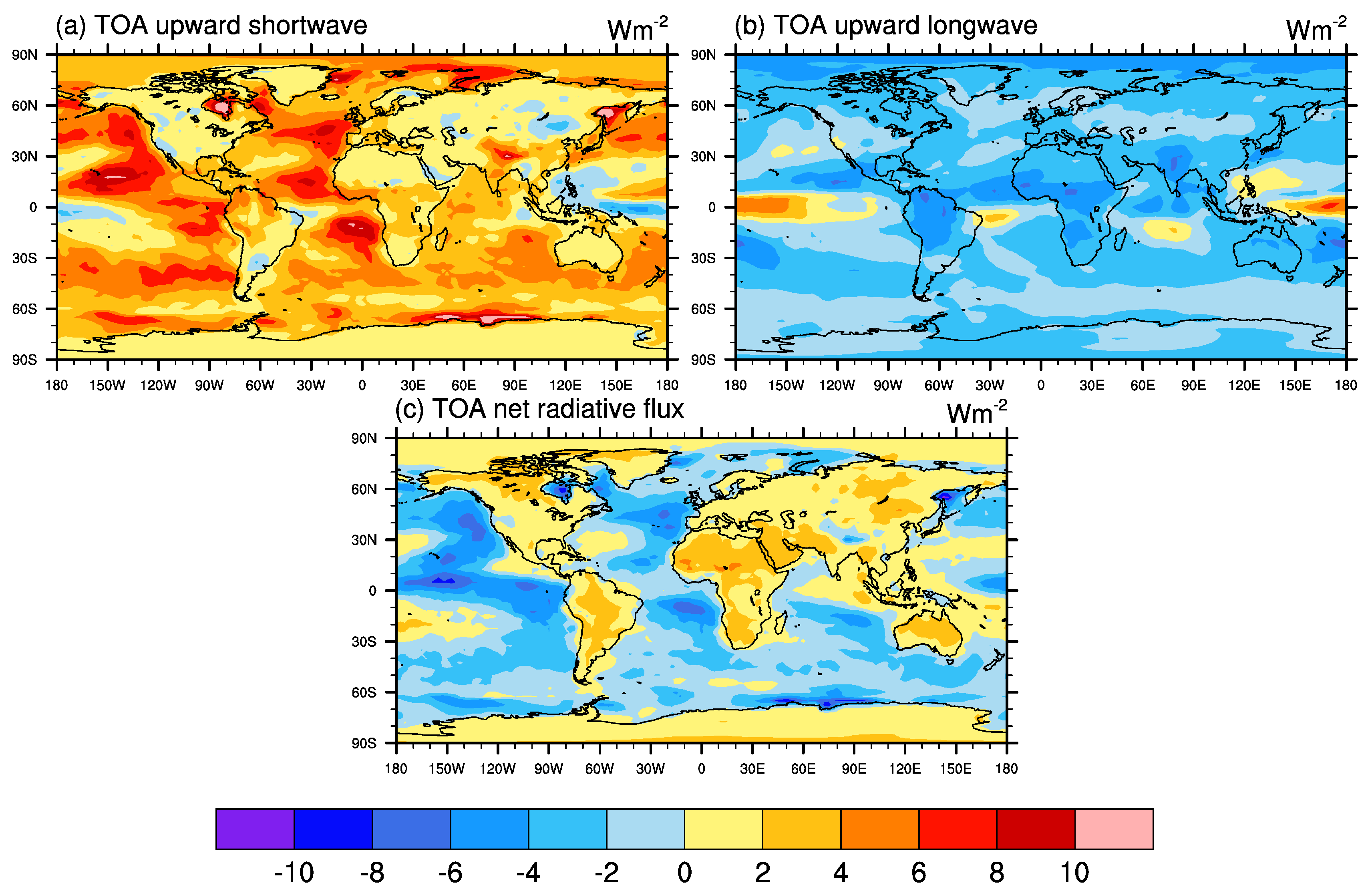
3.1. Radiation Budget at TOA

As the G4cdnc experiment simulates the increase in the reflection of solar radiation by marine clouds, we first examined the changes in the radiation budget at the top of the atmosphere (TOA), expecting an increase in upward shortwave radiation. Figure 1 shows the global distributions of the differences in radiative fluxes at the TOA between G4cdnc and the RCP4.5 experiments during the progress period. During this period, the upward shortwave radiation at the TOA increased by 2.95 Wm⁻² in the global mean multi-model ensemble average. Although there was a decrease in certain areas, especially in the western equatorial Pacific, the reflection of solar radiation was increased overall around the globe with a large increase over the eastern parts of the Pacific and Atlantic Oceans (Figure 1a).

Except for some areas of the inter-tropical convergence zone (ITCZ), the overall increase in reflective shortwave radiation at the TOA resulted in a decrease in outgoing longwave radiation (OLR) at the TOA, indicating a surface cooling not only over the global ocean but over the global land (Figure 1b). A significant decrease in OLR over tropical rainforest regions including the Amazon, equatorial Africa, and the Indo-Pakistan region is noteworthy. In the global mean and multi-model ensemble average, the reduction of OLR (−2.27 Wm⁻²) largely compensates the energy loss by the shortwave reflection.

Overall, the changes in the upward shortwave radiation and OLR tend to compensate each other. Nevertheless, the net radiation at the TOA (net shortwave radiation minus OLR) decreased largely over the oceans, except for the ITCZ area and an increased OLR and Arctic sea-ice region, and increased over most of the land areas, except for the Tibetan Plateau where the upward shortwave radiation significantly increased, unlike the other land areas (Figure 1c). The global mean multi-model ensemble average of the net radiation at the TOA is −0.68 Wm⁻² with a downward positive sign during the progress period. This amount of change in the net radiation corresponds to a 15% reduction of the radiative forcing (4.5 Wm⁻²) induced by anthropogenic activities under the RCP4.5 scenario.

Other than the sea-ice/snow albedo feedback effect, the heterogeneity in regional responses to G4cdnc can also be explained by the changes in cloudiness, soil moisture, and other climate variables, but further investigation into the subject is beyond the scope of this paper.

The differences in the TOA radiation fluxes are replicated in Figure 2 and focused on East Asia, the analysis domain for this study. The marine cloud brightening increased the reflection of shortwave radiation at the TOA over most of the domain but caused a significant decrease over the Gobi Desert area (Figure 2a). There was a considerable increase over the Sea of Okhotsk, which can be related to a positive sea ice–albedo feedback. The increase over Southern China and the Tibetan Plateau can also be related to a positive snow–albedo feedback (figures are not shown). Meanwhile, OLR decreased over most of the domain area even in the area with a decreased shortwave reflection at the TOA (Figure 2b). This reduction of OLR induced by the marine cloud brightening resulted in an increase in downward net radiation at the TOA except for the Sea of Okhotsk and Tibetan Plateau areas (Figure 2c).

3.2. Mean Temperature

To check whether the global warming effect under the RCP4.5 scenario has been alleviated over East Asia through the radiative forcing changes induced by the marine cloud brightening, probability distribution functions (PDFs) for surface air mean temperature are shown in Figure 3 for each of the five models as well as their ensemble mean, using standarized monthly mean anomalies throughout the given periods. In the figure, the PDFs from the progress period of the G4cdnc and RCP4.5 results are compared with the baseline (the base period RCP4.5) results.

In Figure 3, the PDFs of the multi-model ensemble mean exhibit a modest increase in mean temperature between G4cdnc and the baseline, indicating warming despite the implementation of the G4cdnc experiment. The PDFs in the progress period, however, show that the distribution mean under G4cdnc is lower than that under RCP4.5 (G4cdnc: 1.206, RCP4.5: 3.469). The difference in PDFs between the G4cdnc and RCP4.5 experiments is statistically significant at the 95% level by the Kolmogorov–Smirnov test. Hence, this feature implies that the G4cdnc experiment significantly alleviates the additional rise in mean temperature caused by the RCP4.5 scenario over East Asia. The mean of the PDFs from all the models under the G4cdnc experiment is lower than of RCP4.5; the CSIRO-Mk3L-1-2 model resulted in the lowest mean of −0.326, and the MIRCO-ESM model resulted in the greatest mean of 1.198.

This cooling effect of mean temperature is consistent with the results of previous studies investigating the effects of other geoengineering experiments. For example, a study conducted by Curry et al. calculated the PDFs, the same as our method but for the globe, and focused on the difference in mean temperature between the GeoMIP G1 and CMIP5 abrupt4xCO₂ experiments [33]. In that study, PDFs obtained from the G1 experiment are located further left compared to the PDFs obtained from the abrupt4xCO₂ experiment, indicating a very high cooling effect caused by the G1 experiment. Ji et al. also calculated PDFs using the same algorithm for the globe and reported the difference between GeoMIP G4 and CMIP5 RCP4.5 [35]. Similarly, in that study, there was a discernable difference between the PDFs from the G4 experiment and those from RCP4.5, representing an alleviation of the increase in mean temperature caused by RCP4.5.

Figure 3 also shows that the variance of the multi-model ensemble mean PDF obtained from the G4cdnc experiment is lower than that from the RCP4.5 experiment (G4cdnc: 1.655, RCP4.5: 2.748), which is consistent with a previous study result for the G1 experiment compared with the CMIP5 abrupt4xCO₂ experiment [33]. A greater variance in PDFs equates to a larger inter-annual variability in the temperature and probably to the more frequent occurrence of extreme temperatures. Assuming the latter case, extreme temperatures under the G4cdnc experiment may occur less frequently than under the RCP4.5 scenario. Most of the models resulted in a lower variance in PDFs under the G4cdnc experiment than under RCP4.5, with the exception of the CSIRO-Mk3L-1-2 model, presenting the opposite. Meanwhile, the skewness of the multi-model ensemble’s PDFs under G4cdnc also decreases slightly compared with that under RCP4.5 (G4cdnc: 0.380, RCP4.5: 0.457).

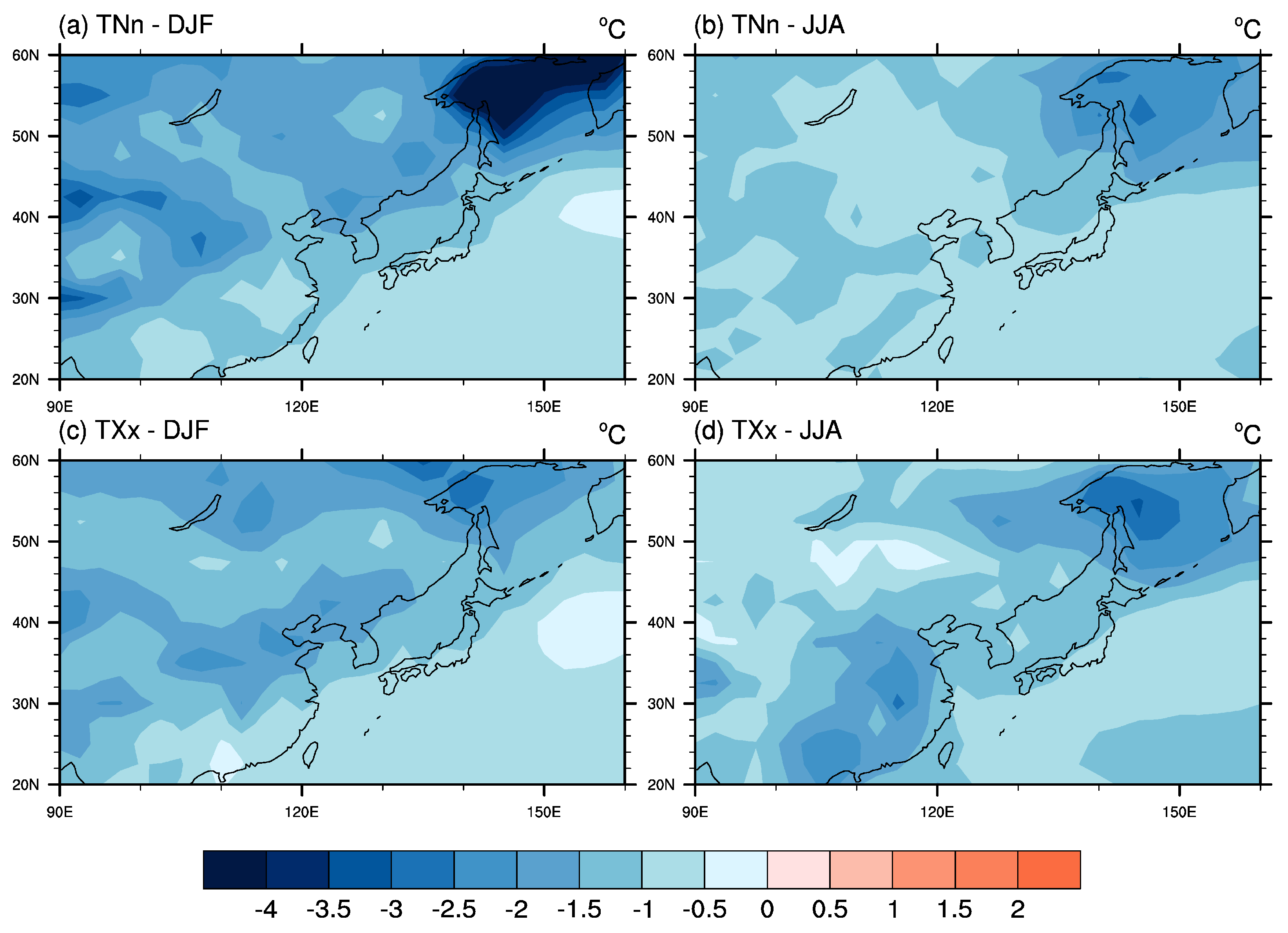
3.3. Temporal and Spatial Response in Extreme Temperatures

To investigate the temporal changes in extreme temperatures over East Asia under the G4cdnc experiment, the differences between G4cdnc and RCP4.5 for the TNn and TXx indices have been analyzed and their time series are shown in Figure 4. Hereafter, ∆ denotes the multi-model ensemble mean of a difference between G4cdnc and RCP4.5 averaged over the progress period (2060–2069).

The results of the G4cdnc experiment are as follows: ∆TNn = −1.128 °C (minimum of −1.695 °C by HadGEM2-ES and maximum of −0.505 °C by CanESM2) and ∆TXx = −0.998 °C (minimum of −1.368 °C by MIROC-ESM and maximum of −0.730 °C by CanESM2). As a result, G4cdnc lowers not only the mean temperature but also extreme temperatures over East Asia by more or less than one degree. Among the models, CanESM2 produced the least change in the extreme temperature indices, which is consistent with the result for mean temperature presented in Section 3.2.

It is notable that the ∆TNn is larger than the ∆TXx, suggesting an implication for extreme cold. Among the extreme temperature studies, many SRM geoengineering studies and studies of other forcing scenarios reported similar results: a larger change in TNn than in TXx (GeoMIP G1 and G4 simulations analyzed by Ji et al., G3 simulation analyzed by Aswathy et al., and studies on simulations under GHG forcing analyzed by Tebaldi et al., Orlowsky and Seneviratne, and Sillmann et al.) [32,34,35,40,41].

Figure 5 shows the geographical distribution of the difference in extreme temperatures between the G4cdnc and RCP4.5 experiments over East Asia during the progress period. The figures demonstrate negative values of ∆TNn and ∆TXx over the entire area of East Asia. However, there appears to be evident regional heterogeneity in the response of extreme temperatures to the G4cdnc simulation.

Notably, the ∆TNn in Figure 5a has a considerably large negative value over the Sea of Okhotsk, lower than −4 °C, whereas ∆TXx has a minimum value of −2 °C over the same region. Several studies noted the larger temperature cooling effect over high-latitude oceanic regions including the Sea of Okhotsk due to SRM geoengineering [35,42,43]. This large temperature response over high-latitude oceanic regions appears to be in line with the well-known global warming effect, polar amplification [44,45,46]. Ji et al. showed that both solar dimming (G1) and stratospheric aerosol (G4) geoengineering resulted in a large ∆TNn over high-latitude oceanic regions in both hemispheres, which was not seen in TXx [35]. It has been found that this high-latitude cooling by geoengineering experiments, such as cloud brightening [42] and solar dimming [43], could restore the sea ice extent to the state of their control experiments.

Although ∆TNn and ∆TXx resulted in cooling all over the area, a land–sea difference of the results is distinct in Figure 5. The G4cdnc experiment has a larger cooling effect of ∆TNn and ∆TXx over the interior of the continent compared to the ocean, with the exception of the Sea of Okhotsk. This land–sea difference in response can also be seen in previous studies that have investigated other geoengineering experiments such as the injection of stratospheric aerosols or marine sea salt [35,47,48]. Alterskjær et al. conducted a model experiment with sea salt injection and showed that the cooling effect in mean temperature is larger over the interior of the continent than in the oceans, except for high-latitude northern hemisphere regions [47]. Volodin et al. and Ji et al. showed a larger cooling effect of stratospheric aerosol injection over tropical and mid-latitude land areas than in the corresponding oceanic areas [35,48].

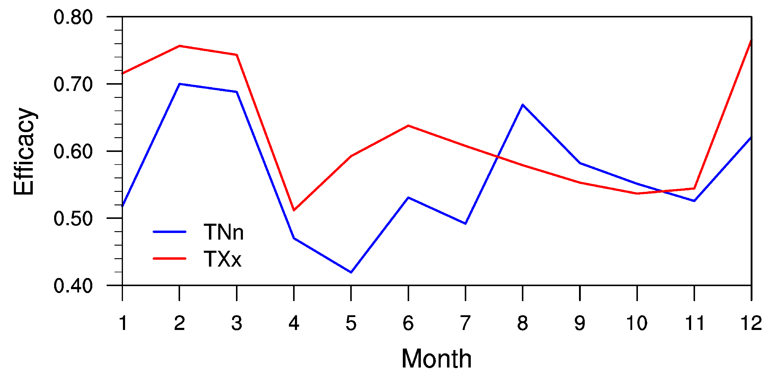
3.4. Seasonality of Extreme Temperature Response

This section examines the effect of seasonality on the changes in the extreme temperature indices, TNn and TXx. To investigate the seasonality, temporal and spatial changes were analyzed and are shown in Figure 6 and Figure 7, respectively, for East Asia in boreal summer and winter during the progress period.

Figure 6 presents the time series for the entire simulation period, but now only the last 10-year averages of the progress period from 2060 to 2069 are used. In both seasons, G4cdnc resulted in cooling of the extreme temperatures. In winter, the multi-model ensemble means of ∆TNn = −1.425 °C and ∆TXx = −1.072 °C are larger than the annual response shown in Figure 4. The inter-model difference is 1.771 °C for TNn, ranging from −2.222 °C to −0.451 °C, and 0.990 °C for TXx, ranging from −1.555 °C to −0.565 °C. These inter-model differences are larger than the annual range. Unlike the winter case, G4cdnc has a larger cooling effect on TXx than on TNn in summer, having multi-model means of ∆TNn = −0.994 °C and ∆TXx = −1.119 °C. The inter-model difference is lower than the annual range: 0.362 °C for TNn, ranging from −1.356 °C to −0.994 °C, and 0.444 for TXx, ranging from −1.458 °C to −1.014 °C. In short, G4cdnc has a greater cooling effect on TNn in winter and on TXx in summer. The inter-model difference for TNn is larger than the ensemble mean annual range during winter, indicating a large uncertainty in simulating the extreme cold.

Figure 7 presents the difference in TNn and TXx between the G4cdnc and RCP4.5 experiments over East Asia in boreal winter and summer during the progress period (2060–2069). The same as the annual case shown in Figure 5, the cooling effect caused by G4cdnc is dominant over the whole of East Asia in both winter and summer. The particularly large cooling effect over the Sea of Okhotsk shown in the annual case for TNn (Figure 5a) does not appear in summer but in winter (Figure 7a,b). An increase in sea ice lowers the air temperature, particularly the minimum temperature [35] and, according to this effect, the G4cdnc experiment demonstrated the largest cooling over the Sea of Okhotsk in winter (Figure 7a). Sea ice in the Sea of Okhotsk varies with season, reaching its maximum in March and minimum in September [49]. Many CMIP5 models projected that the extent of Arctic sea ice will decline under a GHG forcing scenario of RCP4.5 in both summer and winter seasons in the future [50]. In the meantime, a study by Moore et al. demonstrated that the G1 scenario restores the extent of Arctic sea ice from conditions under the high GHG scenario to a preindustrial state [43]. Because of the removal of snow and sea ice in summer, the TNn response to the G4cdnc experiment is weaker in summer over the East Asian continent and the Sea of Okhotsk compared to winter (Figure 7b). The sea ice over the Sea of Okhotsk also causes a larger TXx cooling compared to the rest of the ocean, but a moderate response compared to the TNn cooling in winter (Figure 7c,d).

The land–sea difference revealed in the annual response of the extreme temperature indices in Figure 5 can also be found in the seasonal responses of TNn, especially in winter. Compared to the oceanic response, the G4cdnc experiment results in a larger cooling effect over the East Asian continent, except for Southern China in winter and summer (Figure 7a,c). This continental region with a larger cooling effect is frequently covered by snow during winter, suggesting snow–albedo feedback. A previous study showed that G3 and G4 geoengineering would restore the snow cover that is reduced by GHG forcing, which decreases the surface-sensible heat flux, raises heat capacity, and thus reduced the sensitivity of temperature to radiative forcing changes [35,51].

Figure 8 shows the difference in snow cover and cloudiness between the G4cdnc and RCP4.5 experiments over East Asia in winter during the progress period, but it has been drawn using only two model outputs (CanESM2 and MIROC-ESM) currently available from the data archive. The pattern of snow cover change with a decrease approximately north of 40° N and an increase in the south is consistent with that of the upward shortwave radiation change at the TOA shown in Figure 2a. This result illustrates positive feedback between snow and albedo. The net incoming solar radiation increases over the northern area and it would warm the atmosphere. Then, the resultant decrease in vertical temperature gradient near the surface can cause a decrease in latent and sensible heat fluxes from the surface, followed by a decrease in cloudiness (Figure 8b) and snowfall, daytime warming, and nighttime cooling of the surface after all. This feedback process can possibly be related to the greater cooling of TNn (Figure 7a) over the northern area with the decreased shortwave flux and the smaller cooling of TXx over the area (Figure 7c). Such positive snow–albedo feedback can be applied to the southern area with the increased upward shortwave radiation with the opposite signs as well.

Such a large response over the continent has been shown not only in GHG forcing experiments but also in other geoengineering experiments. Orlowsky and Seneviratne and Sillmann et al. showed that the response of extreme temperatures is projected to be larger over mid- and high-latitude continental bands during winter under CMIP3 and CMIP5 GHG forcing scenarios, respectively [32,41]. Ji et al. showed that G1 and G4 geoengineering experiments have more significant effects over continental land masses of the same latitudinal band compared to those of the ocean [35].

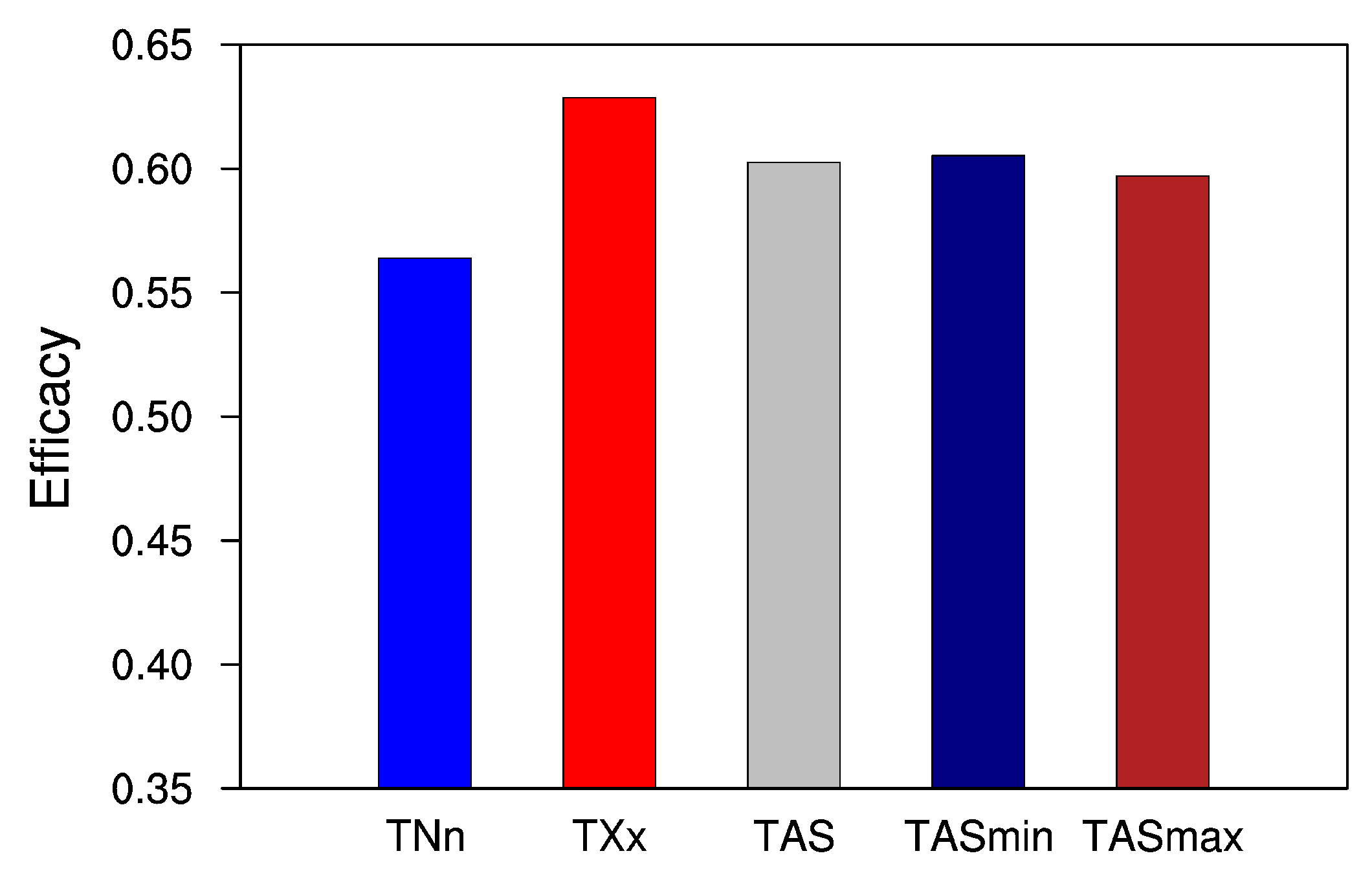
3.5. Relative Effect of Extreme Temperature

We calculated annual and monthly efficacies based on root mean square (RMS) differences to investigate the relative effect on extreme temperatures of the G4cdnc experiment over East Asia. The annual efficacies of extreme temperatures (TNn and TXx) and mean temperatures (TAS, TASmin, and TASmax) are shown in Figure 9, and seasonal variations in efficacy are displayed using monthly values in Figure 10. In this section, we refer to the efficacy in terms of percentages.

The annual efficacies of G4cdnc for decreasing the warming of TNn and TXx under the RCP4.5 conditions in the multi-model ensemble mean over East Asia are 56.6% and 63.4%, respectively. In other words, the efficacy of TXx is larger than that of TNn by 7%, which implies that marine cloud brightening is a relatively effective method of alleviating the warming of TXx compared to TNn under GHG forcing. This asymmetric relative effect on extreme temperatures is the opposite to that represented by the absolute effect on extreme temperatures (∆TNn ≥ ∆TXx in Section 3.3). However, Curry et al., for G1 over the globe, showed that the difference between the efficacies of TNn and TXx is not significant (TNn: 87% and TXx: 89%) [33]. Therefore, the relative effect of marine cloud brightening over East Asia has a different asymmetry from that reported by the G1 experiment. Meanwhile, the annual efficacy for mean temperature over the progress period by the G4cdnc simulation is 60.9% for TAS, 61% for TASmin, and 60.4% for TASmax, which implies that G4cndc is similarly effective in alleviating the warming of the mean temperature. In addition, the efficacies for all mean temperatures are larger than that for TNn but lower than that for TXx.

The monthly efficacy was investigated for extreme temperatures during the progress period (Figure 10). The efficacy of TXx was larger than that of TNn during all the months, except from August to October. The relative effect of TXx reached its maxima of 75% in December to March and its minima of 55% in April and September to November. The efficacy, however, rebounded to 65% from May to July, despite this being during the minima period. The relative effect of TXx shown by the G4cdnc experiment demonstrated a seasonal response; it reached maxima during winter and minima during spring and fall. On the other hand, the relative effect of TNn reached its maxima of 65% in February, March, August, and December and its minima of 50% in the other months. Hence, the relative effect of TNn revealed its double maximum peaks in February and August and its minimum in May, showing relatively low efficacies in spring and fall. In short, the relative effect of extreme temperatures produced by the G4cdnc experiment demonstrates seasonal dependency over East Asia, and the range between the maximum and minimum efficacies reaches up to 30%.

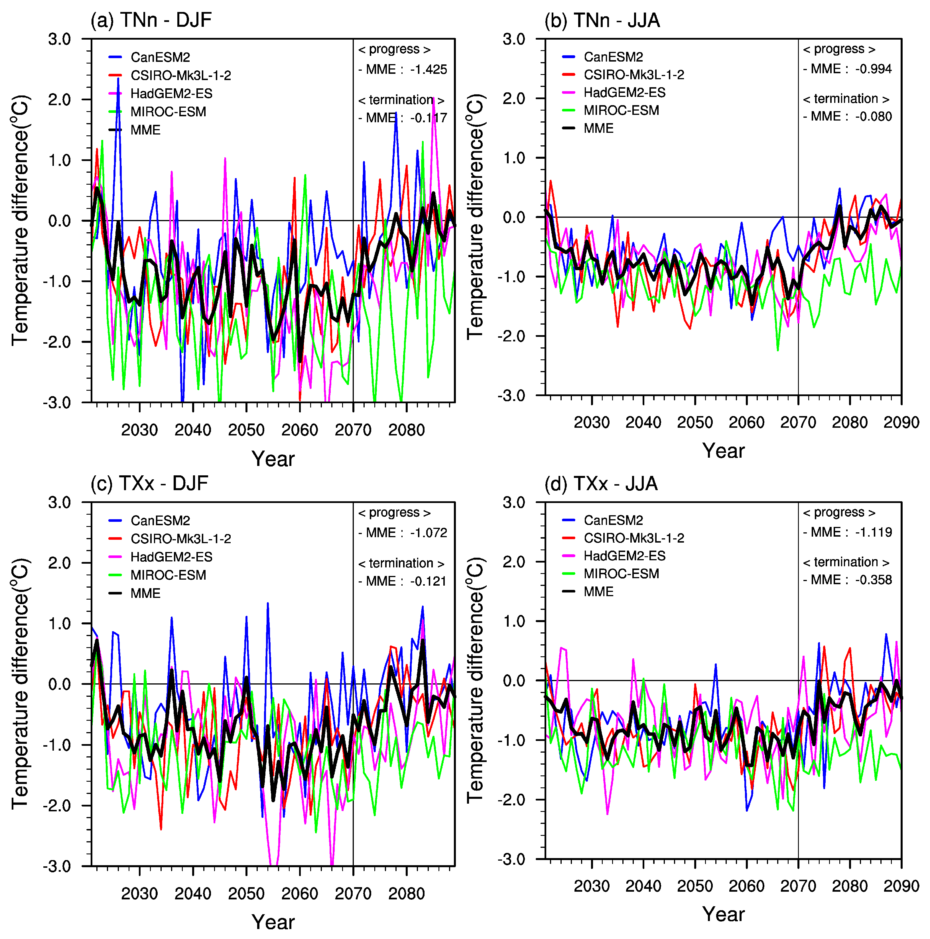
3.6. Durability of Effects after the Termination of G4cdnc

The last 20-year simulation period (2071 to 2090) highlights the consequences of terminating marine cloud brightening after the restoration of CDNC, and the termination period has been specified as the latter 10 years (2081–2090) in this study. Here, we analyze the changes in TNn and TXx indices over East Asia during the termination period, whereas previous studies have researched changes in mean temperatures [4,47,52] after impeding other geoengineering experiments over the globe.

The multi-model ensemble mean of differences in extreme temperatures between the G4cdnc and RCP4.5 experiments over East Asia during the termination period shown in Figure 4 are ∆TNn = −0.321 °C for TNn with an inter-model range of −0.366 °C to −0.255 °C and ∆TXx = −0.278 °C for TXx with a range of −0.417 °C to −0.013 °C. Although the 10-year averaged values of TNn and TXx are still lower than the values under the RCP4.5 experiment, the year-to-year values asymptote to the RCP4.5 level till 2090, the last simulation year of the experiment. This termination effect on extreme temperatures was examined in a previous study that showed a 10th percentile global temperature increase of 0.61 °C and 90th percentile increase of 0.59 °C after shutting down injections of sea salt into the tropical marine atmospheric boundary layer [34]. In the MIROC-ESM model, which did not simulate the termination effect, the values of ∆TNn and ∆TXx remained at around −1 °C during the termination period.

Figure 11 shows the difference pattern of extreme temperatures between the G4cdnc and RCP4.5 experiments over East Asia averaged during the termination period. Both ∆TNn and ∆TXx increased and approached the RCP4.5 results compared to the differences obtained from the progress period. Other studies also presented an increase in extreme temperature over the globe after terminating the forcing of their geoengineering methods [34,47]. It is noteworthy that while the cloud brightening control was implemented in the G4cdnc experiment, the extreme temperatures remained cooler than the RCP4.5 experiment results over the whole East Asian region, but after the termination of the control showing restoration of the experimental forcing CDNC, they increased and, in some regions, showed higher temperature values than the RCP4.5 results. These regionally different responses can cause a political problem between the countries taking control and other countries not participating in the control experiment.

Finally, Figure 12 shows the monthly efficacy of the G4cdnc experiment for extreme temperatures over East Asia during the termination period. As the G4cndc is terminated, the relative effects on both TNn and TXx also decreased significantly. Moreover, the relative effect on TNn during the termination period is larger than TXx in all months except for February, March, and November. For TNn, the efficacy reached its maxima of 15% on average in March and November and its minima of 5% in the rest of the months. TXx reached its maxima of 20% on average in May to August and December and minima of 5% in January to April. In short, the relative effect on extreme temperature during the termination period also shows a seasonal variation but with much weaker seasonality than that during the progress period.

4. Summary and Conclusions

We have investigated the marine cloud brightening effects on extreme temperature indices, TNn and TXx, over East Asia by the GeoMIP Phase 2 G4cdnc experiment under the RCP4.5 warming scenario. For this study, we used five climate model datasets that participated in the G4cdnc experiment and analyzed their multi-model ensemble mean and the individual model results.

Through a brief analysis of the radiation fluxes at the TOA, our results confirmed that the marine cloud brightening could increase the reflection of shortwave radiation at the TOA and decrease the outgoing longwave radiation, resulting in a net radiation loss over ocean and a gain over land, largely compensating the loss in East Asia. Our results also confirmed the sea–ice albedo feedback over ocean, especially over the Sea of Okhotsk and the snow albedo feedback could be a crucial factor determining the radiation response at the TOA in East Asia.

The G4cdnc experiment shows the capability of counteracting the warming of extreme temperatures as well as the mean temperature under the RCP4.5 scenario, though the amount was insufficient to remove the warming to the level of the base period (2006–2019). The efficacy of the cloud control for mean temperature reaches approximately 60%, which is a middle of the efficacies for extreme temperatures: 56% for TNn and 63% for TXx annually. The efficacies for the extreme temperatures revealed a significant seasonality, showing the highest efficacy in winter and relatively low efficacies in spring and fall during the progress period (2060–2069).

Although the cloud control was implemented over ocean only, the changes in the extreme temperatures were larger over land than over ocean in East Asia. The considerable cooling of TNn over the Sea of Okhotsk in winter implies the restoration of the extent of sea ice by the G4cdnc experiment. These findings need to be highlighted since the extent of sea ice has a great influence on the wintertime temperature in mid-latitude land areas of the Northern Hemisphere. It is also probable that the significant cooling of TNn in winter can be related to the increase in wintertime cold events.

In the context that extreme cold events as well as hot spells have occurred more frequently under global warming, how these findings can be used to act on severe weather events is an important issue to be answered prior to any implementation of the cloud control experiment in reality. Thus, more in-depth analysis on the extreme values not only for temperature but also other variables is required on a regional scale. The authors expect this study can be a trigger for these further studies.

References

1. Sanderson, B.M.; O’Neill, B.C.; Tebaldi, C. What would it take to achieve the Paris temperature targets? Geophys. Res. Lett. 2016, 43, 7133–7142. [Google Scholar] [CrossRef]
2. Yang, H.; Dobbie, S.; Ramirez-Villegas, J.; Feng, K.; Challinor, A.J.; Chen, B.; Gao, Y.; Lee, L.; Yin, Y.; Sun, L.; et al. Potential negative consequences of geoengineering on crop production: A study of Indian groundnut. Geophys. Res. Lett. 2016, 43, 11786–11795. [Google Scholar] [CrossRef] [PubMed] [Green Version]
3. Bellamy, R.; Lezaun, J.; Palmer, J. Public perceptions of geoengineering research governance: An experimental deliberative approach. Glob. Environ. Chang. 2017, 45, 194–202. [Google Scholar] [CrossRef]
4. Trisos, C.H.; Amatulli, G.; Gurevitch, J.; Robock, A.; Xia, L.; Zambri, B. Potentially dangerous consequences for biodiversity of solar geoengineering implementation and termination. Nat. Ecol. Evol. 2018, 2, 475–482. [Google Scholar] [CrossRef] [PubMed]
5. Mautner, M. A Space-Based Solar Screen against Climatic Warming. J. Br. Interplanet. Soc. 1991, 44, 135–148. [Google Scholar]
6. Budyko, M.I. On present-day climatic changes. Tellus 1977, 29, 193–204. [Google Scholar] [CrossRef]
7. Crutzen, P.J. Albedo Enhancement by Stratospheric Sulfur Injections: A Contribution to Resolve a Policy Dilemma? Clim. Chang. 2006, 77, 211. [Google Scholar] [CrossRef] [Green Version]
8. Latham, J. Control of global warming? Nature 1990, 347, 339–340. [Google Scholar] [CrossRef]
9. Bala, G.; Duffy, P.B.; Taylor, K.E. Impact of geoengineering schemes on the global hydrological cycle. Proc. Natl. Acad. Sci. USA 2008, 105, 7664–7669. [Google Scholar] [CrossRef] [Green Version]
10. Lenton, T.M.; Vaughan, N.E. The radiative forcing potential of different climate geoengineering options. Atmos. Chem. Phys. 2009, 9, 5539–5561. [Google Scholar] [CrossRef] [Green Version]
11. Irvine, P.J.; Ridgwell, A.; Lunt, D.J. Assessing the regional disparities in geoengineering impacts. Geophys. Res. Lett. 2010, 37, L18702. [Google Scholar] [CrossRef] [Green Version]
12. Kravitz, B.; Robock, A.; Boucher, O.; Schmidt, H.; Taylor, K.E.; Stenchikov, G.; Schulz, M. The Geoengineering Model Intercomparison Project (GeoMIP). Atmos. Sci. Lett. 2011, 12, 162–167. [Google Scholar] [CrossRef]
13. Kravitz, B.; Forster, P.M.; Jones, A.; Robock, A.; Alterskjær, K.; Boucher, O.; Jenkins, A.K.L.; Korhonen, H.; Kristjánsson, J.E.; Muri, H.; et al. Sea spray geoengineering experiments in the geoengineering model intercomparison project (GeoMIP): Experimental design and preliminary results. J. Geophys. Res. Atmos. 2013, 118, 11175–11186. [Google Scholar] [CrossRef] [Green Version]
14. Twomey, S. Pollution and the planetary albedo. Atmos. Environ. 1974, 8, 1251–1256. [Google Scholar] [CrossRef]
15. Stjern, C.W.; Muri, H.; Ahlm, L.; Boucher, O.; Cole, J.N.S.; Ji, D.; Jones, A.; Haywood, J.; Kravitz, B.; Lenton, A.; et al. Response to marine cloud brightening in a multi-model ensemble. Atmos. Chem. Phys. 2018, 18, 621–634. [Google Scholar] [CrossRef] [Green Version]
16. Sillmann, J.; Kharin, V.V.; Zhang, X.; Zwiers, F.W.; Bronaugh, D. Climate extremes indices in the CMIP5 multimodel ensemble: Part 1. Model evaluation in the present climate. J. Geophys. Res. Atmos. 2013, 118, 1716–1733. [Google Scholar] [CrossRef]
17. Kharin, V.V.; Zwiers, F.W. Changes in the Extremes in an Ensemble of Transient Climate Simulations with a Coupled Atmosphere–Ocean GCM. J. Clim. 2000, 13, 3760–3788. [Google Scholar] [CrossRef]
18. Kharin, V.V.; Zwiers, F.W. Estimating Extremes in Transient Climate Change Simulations. J. Clim. 2005, 18, 1156–1173. [Google Scholar] [CrossRef]
19. Easterling, D.R.; Kunkel, K.E.; Wehner, M.F.; Sun, L. Detection and attribution of climate extremes in the observed record. Weather Clim. Extrem. 2016, 11, 17–27. [Google Scholar] [CrossRef] [Green Version]
20. Boo, K.-O.; Kwon, W.-T.; Baek, H.-J. Change of extreme events of temperature and precipitation over Korea using regional projection of future climate change. Geophys. Res. Lett. 2006, 33, L01701. [Google Scholar] [CrossRef]
21. Park, C.; Min, S.-K.; Lee, D.; Cha, D.-H.; Suh, M.-S.; Kang, H.-S.; Hong, S.-Y.; Lee, D.-K.; Baek, H.-J.; Boo, K.-O.; et al. Evaluation of multiple regional climate models for summer climate extremes over East Asia. Clim. Dyn. 2016, 46, 2469–2486. [Google Scholar] [CrossRef]
22. Li, D.; Zhou, T.; Zou, L.; Zhang, W.; Zhang, L. Extreme High-Temperature Events Over East Asia in 1.5 °C and 2 °C Warmer Futures: Analysis of NCAR CESM Low-Warming Experiments. Geophys. Res. Lett. 2018, 45, 1541–1550. [Google Scholar] [CrossRef] [Green Version]
23. Xu, Y.; Gao, X.; Giorgi, F.; Zhou, B.; Shi, Y.; Wu, J.; Zhang, Y. Projected Changes in Temperature and Precipitation Extremes over China as Measured by 50-yr Return Values and Periods Based on a CMIP5 Ensemble. Adv. Atmos. Sci. 2018, 35, 376–388. [Google Scholar] [CrossRef]
24. Taylor, K.E.; Stouffer, R.J.; Meehl, G.A. An Overview of CMIP5 and the Experiment Design. Bull. Am. Meteorol. Soc. 2012, 93, 485–498. [Google Scholar] [CrossRef] [Green Version]
25. Ji, D.; Wang, L.; Feng, J.; Wu, Q.; Cheng, H.; Zhang, Q.; Yang, J.; Dong, W.; Dai, Y.; Gong, D.; et al. Description and basic evaluation of Beijing Normal University Earth System Model (BNU-ESM) version 1. Geosci. Model Dev. 2014, 7, 2039–2064. [Google Scholar] [CrossRef] [Green Version]
26. Arora, V.K.; Scinocca, J.F.; Boer, G.J.; Christian, J.R.; Denman, K.L.; Flato, G.M.; Kharin, V.V.; Lee, W.G.; Merryfield, W.J. Carbon emission limits required to satisfy future representative concentration pathways of greenhouse gases. Geophys. Res. Lett. 2011, 38, L05805. [Google Scholar] [CrossRef]
27. Phipps, S.J.; Rotstayn, L.D.; Gordon, H.B.; Roberts, J.L.; Hirst, A.C.; Budd, W.F. The CSIRO Mk3L climate system model version 1.0—Part 1: Description and evaluation. Geosci. Model Dev. 2011, 4, 483–509. [Google Scholar] [CrossRef] [Green Version]
28. Collins, W.J.; Bellouin, N.; Doutriaux-Boucher, M.; Gedney, N.; Halloran, P.; Hinton, T.; Hughes, J.; Jones, C.D.; Joshi, M.; Liddicoat, S.; et al. Development and evaluation of an Earth-System model—HadGEM2. Geosci. Model Dev. 2011, 4, 1051–1075. [Google Scholar] [CrossRef] [Green Version]
29. Watanabe, S.; Hajima, T.; Sudo, K.; Nagashima, T.; Takemura, T.; Okajima, H.; Nozawa, T.; Kawase, H.; Abe, M.; Yokohata, T.; et al. MIROC-ESM 2010: Model description and basic results of CMIP5-20c3m experiments. Geosci. Model Dev. 2011, 4, 845–872. [Google Scholar] [CrossRef] [Green Version]
30. Zhang, X.; Alexander, L.; Hegerl, G.C.; Jones, P.; Tank, A.K.; Peterson, T.C.; Trewin, B.; Zwiers, F.W. Indices for monitoring changes in extremes based on daily temperature and precipitation data. Wires Clim. Chang. 2011, 2, 851–870. [Google Scholar] [CrossRef]
31. Donat, M.G.; Alexander, L.V.; Yang, H.; Durre, I.; Vose, R.; Caesar, J. Global Land-Based Datasets for Monitoring Climatic Extremes. Bull. Am. Meteorol. Soc. 2013, 94, 997–1006. [Google Scholar] [CrossRef] [Green Version]
32. Orlowsky, B.; Seneviratne, S.I. Global changes in extreme events: Regional and seasonal dimension. Clim. Chang. 2012, 110, 669–696. [Google Scholar] [CrossRef] [Green Version]
33. Curry, C.L.; Sillmann, J.; Bronaugh, D.; Alterskjaer, K.; Cole, J.N.S.; Ji, D.; Kravitz, B.; Kristjánsson, J.E.; Moore, J.C.; Muri, H.; et al. A multimodel examination of climate extremes in an idealized geoengineering experiment. J. Geophys. Res. Atmos. 2014, 119, 3900–3923. [Google Scholar] [CrossRef] [Green Version]
34. Aswathy, V.N.; Boucher, O.; Quaas, M.; Niemeier, U.; Muri, H.; Mülmenstädt, J.; Quaas, J. Climate extremes in multi-model simulations of stratospheric aerosol and marine cloud brightening climate engineering. Atmos. Chem. Phys. 2015, 15, 9593–9610. [Google Scholar] [CrossRef] [Green Version]
35. Ji, D.; Fang, S.; Curry, C.L.; Kashimura, H.; Watanabe, S.; Cole, J.N.S.; Lenton, A.; Muri, H.; Kravitz, B.; Moore, J.C. Extreme temperature and precipitation response to solar dimming and stratospheric aerosol geoengineering. Atmos. Chem. Phys. 2018, 18, 10133–10156. [Google Scholar] [CrossRef] [Green Version]
36. Jones, P.W. First- and Second-Order Conservative Remapping Schemes for Grids in Spherical Coordinates. Mon. Weather Rev. 1999, 127, 2204–2210. [Google Scholar] [CrossRef]
37. Schmidt, H.; Alterskjær, K.; Bou Karam, D.; Boucher, O.; Jones, A.; Kristjánsson, J.E.; Niemeier, U.; Schulz, M.; Aaheim, A.; Benduhn, F.; et al. Solar irradiance reduction to counteract radiative forcing from a quadrupling of CO2: Climate responses simulated by four earth system models. Earth Syst. Dyn. 2012, 3, 63–78. [Google Scholar] [CrossRef] [Green Version]
38. Haigh, J.; Conover, W.J. Practical Nonparametric Statistics. J. R. Stat. Soc. Ser. A (Gen.) 1981, 3, 370–371. [Google Scholar] [CrossRef]
39. Kravitz, B.; Caldeira, K.; Boucher, O.; Robock, A.; Rasch, P.J.; Alterskjær, K.; Karam, D.B.; Cole, J.N.S.; Curry, C.L.; Haywood, J.M.; et al. Climate model response from the Geoengineering Model Intercomparison Project (GeoMIP). J. Geophys. Res. Atmos. 2013, 118, 8320–8332. [Google Scholar] [CrossRef]
40. Tebaldi, C.; Hayhoe, K.; Arblaster, J.M.; Meehl, G.A. Going to the Extremes. Clim. Chang. 2006, 79, 185–211. [Google Scholar] [CrossRef]
41. Sillmann, J.; Kharin, V.V.; Zwiers, F.W.; Zhang, X.; Bronaugh, D. Climate extremes indices in the CMIP5 multimodel ensemble: Part 2. Future climate projections. J. Geophys. Res. Atmos. 2013, 118, 2473–2493. [Google Scholar] [CrossRef]
42. Rasch, P.J.; Latham, J.; Chen, C.C.J. Geoengineering by cloud seeding: Influence on sea ice and climate system. Environ. Res. Lett. 2009, 4, 045112. [Google Scholar] [CrossRef]
43. Moore, J.C.; Rinke, A.; Yu, X.; Ji, D.; Cui, X.; Li, Y.; Alterskjær, K.; Kristjánsson, J.E.; Muri, H.; Boucher, O.; et al. Arctic sea ice and atmospheric circulation under the GeoMIP G1 scenario. J. Geophys. Res. Atmos. 2014, 119, 567–583. [Google Scholar] [CrossRef] [Green Version]
44. Holland, M.M.; Bitz, C.M. Polar amplification of climate change in coupled models. Clim. Dyn. 2003, 21, 221–232. [Google Scholar] [CrossRef]
45. Bekryaev, R.V.; Polyakov, I.V.; Alexeev, V.A. Role of Polar Amplification in Long-Term Surface Air Temperature Variations and Modern Arctic Warming. J. Clim. 2010, 23, 3888–3906. [Google Scholar] [CrossRef]
46. Pithan, F.; Mauritsen, T. Arctic amplification dominated by temperature feedbacks in contemporary climate models. Nat. Geosci. 2014, 7, 181–184. [Google Scholar] [CrossRef]
47. Alterskjær, K.; Kristjánsson, J.E.; Boucher, O.; Muri, H.; Niemeier, U.; Schmidt, H.; Schulz, M.; Timmreck, C. Sea-salt injections into the low-latitude marine boundary layer: The transient response in three Earth system models. J. Geophys. Res. Atmos. 2013, 118, 12195–12206. [Google Scholar] [CrossRef] [Green Version]
48. Volodin, E.M.; Kostrykin, S.V.; Ryaboshapko, A.G. Climate response to aerosol injection at different stratospheric locations. Atmos. Sci. Lett. 2011, 12, 381–385. [Google Scholar] [CrossRef]
49. Zhao, P.; Zhang, X.; Zhou, X.; Ikeda, M.; Yin, Y. The Sea Ice Extent Anomaly in the North Pacific and Its Impact on the East Asian Summer Monsoon Rainfall. J. Clim. 2004, 17, 3434–3447. [Google Scholar] [CrossRef]
50. Stroeve, J.C.; Serreze, M.C.; Holland, M.M.; Kay, J.E.; Malanik, J.; Barrett, A.P. The Arctic’s rapidly shrinking sea ice cover: A research synthesis. Clim. Chang. 2012, 110, 1005–1027. [Google Scholar] [CrossRef] [Green Version]
51. Berdahl, M.; Robock, A.; Ji, D.; Moore, J.C.; Jones, A.; Kravitz, B.; Watanabe, S. Arctic cryosphere response in the Geoengineering Model Intercomparison Project G3 and G4 scenarios. J. Geophys. Res. Atmos. 2014, 119, 1308–1321. [Google Scholar] [CrossRef]
52. Jones, A.; Haywood, J.M.; Alterskjær, K.; Boucher, O.; Cole, J.N.S.; Curry, C.L.; Irvine, P.J.; Ji, D.; Kravitz, B.; Kristjánsson, J.E.; et al. The impact of abrupt suspension of solar radiation management (termination effect) in experiment G2 of the Geoengineering Model Intercomparison Project (GeoMIP). J. Geophys. Res. Atmos. 2013, 118, 9743–9752. [Google Scholar] [CrossRef] [Green Version]
Figure 1. Geographical distribution of the difference of (a) top of the atmosphere (TOA) upward shortwave radiation, (b) TOA upward longwave radiation, and (c) TOA net radiative flux between G4cdnc and RCP4.5 during the progress period. Results are shown for multi-model ensemble mean.
Atmosphere 11 01345 g001
Figure 2. (a) top of the atmosphere (TOA) upward shortwave radiation, (b) TOA upward longwave radiation, and (c) TOA net radiative flux between G4cdnc and RCP4.5 during the progress period. Results are shown for multi-model ensemble mean, over East Asia.
Atmosphere 11 01345 g002
Figure 3. Probability distributions of standardized monthly mean anomalies for three experiments: G4cdnc (blue), RCP4.5 (red), and base period RCP4.5 (black). Probability density functions (PDFs) are over East Asia during the progress period (year 2060 to 2069). Anomalies are calculated with respect to the mean and standard deviation of the base period for the RCP4.5 scenario for each experiment. “False” shown in the upper right corner indicates that the difference in the distribution between G4cdnc and RCP4.5 is significant at the 95% level by the Kolmogorov–Smirnov test and “True” indicates vice versa.
Atmosphere 11 01345 g003
Figure 4. Timeseries of the difference in extreme temperature indices between G4cdnc and RCP4.5 over East Asia. The timeseries shows the differences in (a) monthly minimum of daily minimum temperature (TNn) and (b) monthly maximum of daily maximum temperature (TXx). The heavy dark curve represents the multi-model ensemble mean of all models used in this study, excluding the MIROC-ESM model. The multi-model ensemble means over the last 10 years for the progress and termination periods are located in upper right corner of each plot.
Atmosphere 11 01345 g004
Figure 5. Geographical distribution of the difference in the extreme temperature indices between the G4cdnc and RCP4.5 simulations during the progress period over East Asia. The distributions show the differences in (a) TNn and (b) TXx. The results are shown for the multi-model ensemble mean.
Atmosphere 11 01345 g005
Figure 6. Time series of the difference in the extreme temperature indices (a,b) TNn and (c,d) TXx between the G4cdnc and RCP4.5 simulations over East Asia for (a,c) December-January-February (DJF) and (b,d) June-July-August (JJA). The heavy dark curve is the multi-model ensemble mean used in this study, excluding the MIROC-ESM model. The multi-model ensemble means for the last 10 years of the progress and termination periods are located in right upper corner of each plot.
Atmosphere 11 01345 g006
Figure 7. Geographical distribution of the difference in extreme temperature indices (a,b) TNn and (c,d) TXx between the G4cdnc and RCP4.5 simulations during the (a,c) DJF and (b,d) JJA seasons in the progress period over East Asia. The results show the multi-model ensemble mean.
Atmosphere 11 01345 g007
Figure 8. Geographical distributions of the differences in (a) snow cover and (b) cloud cover between the G4cdnc and RCP4.5 simulations during DJF season in the progress period over East Asia. The results are derived from two models of CanESM2 and MIROC-ESM.
Atmosphere 11 01345 g008
Figure 9. Annual efficacy of the G4cdnc experiment for neutralizing extreme (TNn and TXx) and daily mean (TAS), daily minimum (TASmin), and daily maximum (TASmax) temperatures in RCP4.5 over East Asia. Results are shown for multi-model ensemble mean.
Atmosphere 11 01345 g009
Figure 10. Timeseries of monthly efficacy of the G4cdnc experiment for neutralizing extreme (TNn and TXx) temperatures during the progress period (2060–2069) in RCP4.5 over East Asia. Results are shown for multi-model ensemble mean.
Atmosphere 11 01345 g010
Figure 11. Geographical distribution of the differences in extreme temperature indices between G4cdnc and RCP4.5 for termination period over East Asia. The distributions show the difference in (a) TNn and (b) TXx. The multi-model mean results are shown, excluding the MIROC-ESM model.
Atmosphere 11 01345 g011
Figure 12. Timeseries of monthly efficacy of the G4cdnc experiment for neutralizing extreme (TNn and TXx) temperatures during the termination period for the RCP4.5 scenario over East Asia. Results are shown for multi-model ensemble mean, excluding MIROC-ESM model.
Atmosphere 11 01345 g012