Article

Pressure-Gradient Forcing Methods for Large-Eddy Simulations of Flows in the Lower Atmospheric Boundary Layer

1
Department of Forest, Grassland and Freshwater Ecology, Unité de Recherche des Forets Méditerranéennes (URFM), French National Institute for Agriculture, Food, and Environment (INRAE), CEDEX 9, 84914 Avignon, France
2
Earth and Environmental Sciences Division, Los Alamos National Lab, Los Alamos, NM 87545, USA
3
Research Applications Laboratory, National Center for Atmospheric Research, Boulder, CO 80301, USA
*
Author to whom correspondence should be addressed.
Atmosphere 2020, 11(12), 1343; https://doi.org/10.3390/atmos11121343
Submission received: 26 October 2020 / Revised: 30 November 2020 / Accepted: 9 December 2020 / Published: 11 December 2020
(This article belongs to the Special Issue Coupled Fire-Atmosphere Simulation)

Abstract

:
Turbulent flows over forest canopies have been successfully modeled using Large-Eddy Simulations (LES). Simulated winds result from the balance between a simplified pressure gradient forcing (e.g., a constant pressure-gradient or a canonical Ekman balance) and the dissipation of momentum, due to vegetation drag. Little attention has been paid to the impacts of these forcing methods on flow features, despite practical challenges and unrealistic features, such as establishing stationary velocity or streak locking. This study presents a technique for capturing the effects of a pressure-gradient force (PGF), associated with atmospheric patterns much larger than the computational domain for idealized simulations of near-surface phenomena. Four variants of this new PGF are compared to existing forcings, for turbulence statistics, spectra, and temporal averages of flow fields. Results demonstrate that most features of the turbulent flow are captured. The variants can either enable modelers to prescribe a wind speed and direction at a reference height close to the ground as required in wildfire simulations, and/or mitigate streaks locking by reproducing the stability of the Ekman balance. Conditions of use, benefits, and drawbacks are discussed. PGF approaches, therefore, provide a viable solution for precursor inflows, including for the specific domains used in fire simulations.

1. Introduction

Turbulent flows over the forest canopy and forest gaps have been studied in wind-tunnel, field, and numerical experiments, leading to a good understanding of turbulence development mechanisms and a better knowledge of turbulence structures in homogeneous canopies and at forest edges [1]. A variety of numerical models are now used to simulate wind fields with a reasonable degree of accuracy. Among the different techniques used to simulate wind flows, one of the most fruitful approaches is the Large-Eddy Simulation (LES), which enables explicit computation of the turbulent structures larger than grid size [2,3,4,5,6,7,8,9,10,11]. This technique has been applied to a wide variety of investigations. For instance, simulations enable researchers to disentangle the mechanisms associated with interactions between canopy and wind flow [7,8] and to determine the spatial extent and other important properties of transition zones in heterogeneous canopies [2,4,9]. They enable simulation of seed [10] and pollen [11] dispersal. In the context of wildfire, they can be used to develop precursor windflows for physics-based-wildfire-behavior modeling (e.g., References [2,3]) or firebrand transport [12], and even to analyze wind measurement accuracy or representativeness in the context of fire experiments [13]. Finally, they help understand discrepancies in observations, e.g., for eddy-covariance measurements [14] or to compute precursor wind flow for wind turbine modeling [15]. The development of resolved canopy-shear-induced turbulence requires fetch distances that are much greater than the desirable domain size for the studies described above (hundreds to thousands of meters). Promising methods based on stochastic perturbations have been proposed to accelerate this transition [16,17], but periodic boundary conditions are still widely used. A periodic domain essentially serves as a Lagrangian window that moves downwind as the shear profile develops and allows the modeler to side-step explicit representation of vast distances (thereby reducing computational resource requirements). The obvious limitation of this approach is that the influences of structures or patterns in the atmosphere that are larger than the domain size are not explicitly represented. Additional steps must be taken to account for the large-scale forcing that counterbalances the momentum sink resulting from vegetation drag in the lower part of the boundary layer. Unfortunately, the existing forcings associated with periodic boundary conditions have some practical limitations under particular configurations. These are detailed below.
Modeling phenomena affected by ambient winds in real events (e.g., reproducing fire experiments [18], particle or scalar dispersion and transport) requires representing the upwind atmospheric conditions. Nudging and data assimilation techniques have been developed to force atmospheric models with meteorological observations at regional (e.g., References [19,20]) or local [21] scales. At the forest canopy or fire experiment scale, observations are often limited to wind speeds and directions at given heights at a limited number of points. Reproducing the real three-dimensional boundary-layer flows is impossible with such limited description, forcing modelers to make assumptions or simplifications in their boundary and initial conditions leading to somewhat idealized simulations. The Ekman balance [22], referred to later as EKB, is the theoretical balance between the mesoscale pressure gradient, the Coriolis force, and the vegetation drag. EKB is quite often used in idealized LES of the atmospheric boundary-layer (e.g., Reference [23]), but far less often for the atmospheric surface layer [9]. The magnitude and direction of this pressure gradient, generally assumed constant, are set according to the expected geostrophic wind. LES of EKB reported streaks [23,24], which are streamwise vortical structures as large as several hundreds of meters, can be observed in the simulated atmospheric boundary-layer [23,25,26]. They build, evolve, and dissipate over periods of several tens of minutes [26,27,28]. With EKB, the wind velocity and direction at a given height close to the canopy depend on vegetation characteristics and the Coriolis parameter, and is only controlled by the geostrophic wind. This is not practical when the reference conditions (wind speed and direction) are only known close to the ground, as in most wildfire or wind energy applications, since the appropriate value for the coinciding geostrophic wind is difficult to determine a priori. Additionally, the rotation with height induced by the Coriolis force complicates the analysis of simulations when vegetation or topography is not homogeneous over the domain. The Coriolis force either supports or destroys the planetary boundary-layer structures, depending on whether their vorticity is parallel or counter parallel to the planetary vorticity [29].
The Coriolis force is neglected in most simulations of the surface-boundary-layer (e.g., References [2,4,7,30,31,32,33]), as well as in many simulations of the atmospheric boundary-layer (e.g., References [34,35,36]). In these simulations, a spatially-constant-pressure-gradient force most often compensates the momentum sink induced by surface roughness elements. Several variants of such a pressure gradient are used among studies cited above. The pressure-gradient can either be constant, or evolve with time to keep the mass flow constant. The forcing can be applied to the whole domain or in the upper part only. This type of forcing, later referred to as CPGF, avoids the complexity induced by the Coriolis-induced spiraling, and is generally presented as a relevant representation of atmospheric surface and boundary-layer flows [34]. However, even if the wind velocity at a given height can be roughly estimated with the law of the wall, it cannot be specified accurately, as for the EKB. Moreover, Reference [31] reported an unusually-large forcing, due to limited domain height and overestimations of the mean streamwise velocity. Regarding applied studies, the streaky structures simulated with CPGF tend to be persistent and “locked”, when domain extents are less than some tens of kilometers [36,37], which is not appropriate in applied canopy flow studies where velocities at specific locations are important, such as wildfire-precursor computations. CPGF is often used in incompressible codes using spectral solvers with a free-slip upper boundary condition. With compressible codes, a frequent alternative to EKB for canopy-flow simulations is the use of a geostrophic wind corresponding to a base state at the top of the domain that drives the flow, in combination with a Rayleigh damping layer (e.g., References [5,6]). This type of forcing is typically used for wildfire simulations, in which domain height is generally large with respect to domain length (to include the plume) and the grid resolution is fine near the ground, although it also leads to streaks locking [2].
This manuscript presents a forcing for capturing the effects of large-scale-pressure-gradient forces that has been developed for wildfire-precursor simulations, to avoid practical limitations of EKB and CPGF. Building on a modified version of CPGF for applied canopy-flow simulations, our approach aims at (1) using a pressure profile closer to the one of the EKB, (2) allowing the forcing of the velocity at a given height, (3) mitigating streak locking in precursor simulations. Here, simulations with various pressure forcing methods are compared to idealized atmospheric boundary-layer simulations, for configurations typically used for precursor computations in wildfire simulations. In addition, the sensitivity to the grid size is investigated in the manuscript, so that the use of the methods to other applications is discussed (canopy flows, idealized boundary-layer research, comparison with observed events or wind turbine simulations).

2. Model Description

2.1. HIGRAD/FIRETEC

The HIGRAD/FIRETEC model is a coupled fire/atmosphere model in which an atmospheric model (HIGRAD [38]) is coupled to a combustion and heat transfer model (FIRETEC [39]), enabling physics-based wildfire simulations (e.g., References [2,18]). HIGRAD solves the compressible Navier-Stokes equations using the method of averages (MOA). The MOA scheme combines and averages the advective tendency, buoyancy, local-pressure-gradient, and Coriolis-force terms of the momentum equations over several small timesteps on the order of a millisecond with a computationally inexpensive first-order accurate scheme. Subsequently, the combined and averaged forces along with averaged advective velocities are used to calculate a larger timestep evolution with an accurate second-order scheme in time and space, yielding numerical damping of sound waves and effective relaxation of Courant condition within the model (see Reference [38] for more details). The vegetation drag formulation is explicitly using a three-dimensional representation of vegetation as porous media. Other details regarding turbulence and drag are described in Reference [6].

2.2. Large-Scale-Pressure Gradient Forces

2.2.1. Background: EKB and CPGF Formulations

For a geostrophic wind of magnitude U g aligned with the x-axis, the momentum equations of the zonal and meridional components of the wind velocity corresponding to EKB can be written:
D u d t = f v 1 ρ d p d x + R x ,
D v d t = f ( U g u ) 1 ρ d p d y + R y ,
In these equations, f v and f u are the components of the Coriolis force, f U g is the mesoscale pressure gradient (Figure 1). ρ , p , R x and R y are, respectively, the air density, the pressure perturbation, and the Reynolds-stress gradient components in the x and y-directions. This formulation can be associated with a capping inversion in ABL simulations.
For a wind aligned with the x-axis, the momentum equations for the zonal and meridional components of the wind velocity corresponding to CPGF can be written:
D u d t = CPGF ( t ) 1 ρ d p d x + R x ,
D v d t = 1 ρ d p d y + R y ,
In Equation (3), CPGF can be a time-dependent function that evolves to conserve the initial momentum with time, thus capturing the natural balance between the large-scale forcing and the vegetation drag. A capping inversion cannot be used with CPGF, since the stable temperature stratification above the inversion prohibits the development of turbulence that should balance the pressure gradient.

2.2.2. Differences of Pressure Profiles and Balance Stability between EKB and CPGF

Regarding EKB, a consequence of the Coriolis force is the well-known rotation of the flow direction as one descends from the upper geostrophic layer to the ground. Combined with the large-scale-pressure-gradient, it also affects the horizontal wind speed, u 2 + v 2 . To estimate this effect, we take the time-derivative of this magnitude:
d u 2 + v 2 d t = 1 u 2 + v 2 ( u d u d t + v d v d t ) ,
Combined with Equations (1) and (2), the contribution of Coriolis and large-scale-pressure gradient to the time-derivative of the horizontal wind speed at a given height is:
1 u 2 + v 2 ( u f v + v f ( U g u ) ) = f v U g u 2 + v 2 ,
The physical meaning of Equation (6) is that the resultant of Coriolis and mesoscale-pressure-gradient forces acts as an effective induced-pressure gradient of magnitude:
1 ρ d P d s = f U g v u 2 + v 2 ,
When the geostrophic wind is aligned with the x-axis, v u 2 + v 2 is the sine of the angle θ between the wind direction and the geostrophic wind (Figure 1). The force per unit mass, due to the Coriolis and mesoscale-pressure-gradient forces (described in Equation (7)) is thus the projection of 1 ρ d P d y = f U g (pressure-gradient force in the y-direction) in the direction of the mean wind at a given height.
v u 2 + v 2 can be approximated using the Ekman spiral ([22], p. 267): u ( z ) = U g ( 1 e γ z cos γ z ) and v ( z ) = U g e γ z sin γ z , with γ = f 2 K and K being an eddy diffusivity. For a geostrophic wind U g along the x-axis, the effect of the projection of the large-scale-pressure-gradient force, F E K B p r o j ( z ) , on wind direction can be written:
F E K B p r o j ( z ) = f U g sin θ ( z ) ,
with
sin θ ( z ) = e γ z sin γ z 1 + e 2 γ z 2 e γ z cos γ z ,
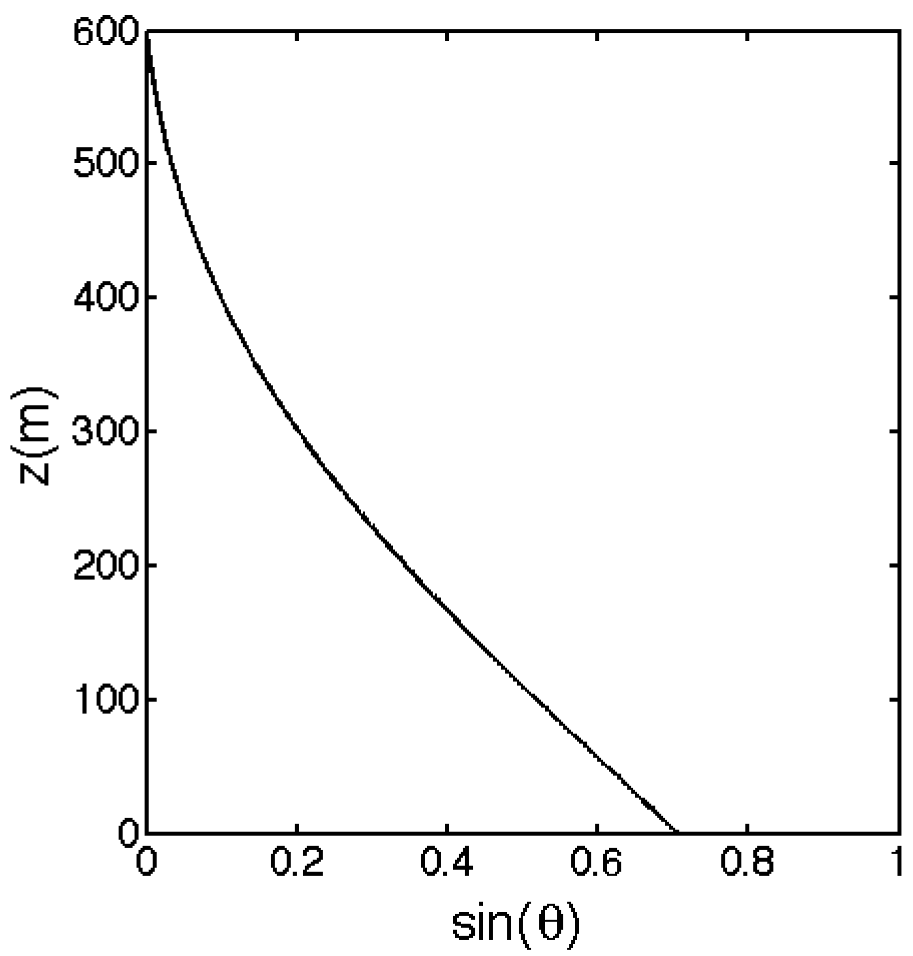
A representation of sin θ ( z ) is shown in Figure 2, assuming a 600-m geostrophic layer ( γ = π 600 ) . This decay of the EKB pressure-gradient magnitude with elevation in the streamwise direction is a major difference between CPGF and EKB. The PGF methods developed in the next subsection implement a pressure-gradient profile closer in magnitude to the EKB than the vertically-constant CPGF, but without the spiraling, which induces practical complexity. Such a formulation can be used with a capping inversion, since the pressure gradient tends to 0 at the top of the geostrophic layer.
In addition to the spiraling and the velocity enhancement, the mesoscale-pressure-gradient and the Coriolis forces also result in a stable equilibrium of mass flow. To demonstrate the stability, let u e q ( z ) and v e q ( z ) be the u and v velocity profiles when the EKB is reached. When v ( z ) is smaller than v e q ( z ) , the forcing on the u velocity is smaller than f v e q , so that u ( z ) becomes smaller than u e q ( z ) . Meanwhile, the forcing on v-velocities becomes greater than f ( U g u e q ( z ) ) , making v ( z ) increase toward v e q ( z ) . The balance deriving from the combination of the mesoscale pressure gradient and the Coriolis force is thus stable. More generally, the Coriolis force affects the coherent statistical structures on a timescale 1 Ω 3 h [29]. The EKB serves a key role in determining the formation or persistence of the streaky structures. The EKB naturally acts to limit streak magnitude, since low and high-speed streaks are steered to the mean EKB profile.
Conversely, the pressure gradient associated with CPGF is spatially homogeneous across a horizontal plane. The mean flow converges at a given height, but there is no mechanism to force the convergence to be uniform at a given (xy) plane, apart from the lateral shear induced by the streaky structure. This single limiting mechanism is insufficient to prevent the locking of persistent streaky structures, that develop when computational domains are not extremely long [36,37]. This weaker convergence is, hence, a second major difference between CPGF and EKB. In the next subsection, descriptions are presented for variations of the PGF formulations that include a mechanism to mimic the stabilization induced by the Coriolis force in the EKB.

2.2.3. Development of the New PGFs (Pressure-Gradient Forces)

As for CPGF (Equation (3)), we propose a dynamic adjustment of the projected pressure force described in Equation (8), replacing the Coriolis parameter f by a function of time F ( t ) :
D u d t = F ( t ) U g sin θ ( z ) 1 ρ d p d x + R x ,
This time-dependent adjustment is determined through a periodic comparison against a target equilibrium state. Let M ( t ) and M e q be the momentum integral over the domain at a given time t and at the equilibrium state, respectively, ( M ( t ) = x , y , z l x l y l z ρ u d x d y d z and M e q = x , y , z l x l y l z ρ u e q d x d y d z ) . Assuming a constant value of the F ( t ) function between t Δ t and t + Δ t , a forecasted momentum integral, M ( t + Δ t ) , can be linearly estimated by extrapolating: M ( t + Δ t ) = 2 M ( t ) M ( t Δ t ) . The modification of F ( t ) ,   Δ F ( t ) , required to make M ( t ) converge toward M e q can thus be derived from the integration over time and space of the momentum equation:
M e q ( 2 M ( t ) M ( t Δ t ) ) Δ t = x , y , z l x l y l z ( F ( t + Δ t ) F ( t ) ) ρ U g sin θ ( z ) d x d y d z ,
So that
Δ F ( t ) = F ( t + Δ t ) F ( t ) =   M e q ( 2 M ( t ) M ( t Δ t ) ) U g Δ t l x l y z l z ρ ( z ) sin θ ( z ) d z ,
where lx and ly are the horizontal length of the domain in the x- and y-direction, respectively. M e q can be estimated from an empirical wind profile (Appendix A).
The combination of Equations (9) and (10) for the PGF formulation and Equation (12) for the update of F(t) every Δ t is later referred to as PGF1 (Table 1). Using PGF1, the integrated momentum is preserved throughout the simulation similarly to CPGF. At the same time, the vertical distribution of the force mimics EKB, but the force is applied in the streamwise direction, which alleviates the complications associated with the spiraling that occurs with the EKB. The appropriate time interval at which F(t) has to be updated, Δ t , is a characteristic time of pressure-gradient action on the mean flow. As shown later, Δ t is chosen much bigger than the computational time step, on the order of 200 s. In the case where a wind flow is desired to be consistent with a target velocity, uref, at a given height, z r e f , a variant of PGF1 is designed to integrate the momentum at zref, instead of over the vertical extent of the domain. Let M r e f ( t ) = x , y l x l y ρ u ( x , y , z r e f ) d x d y and M e q r e f = l x l y ρ r e f u r e f , where ρ r e f is air density at reference height. We can update F ( t ) using the following equation:
Δ F ( t ) = ρ l x l y u r e f ( 2 M r e f ( t ) M r e f ( t Δ t ) ) U g Δ t l x l y sin θ ( z r e f ) ρ r e f ,
With this scheme, the integrated momentum M r e f ( t ) converges toward M e q r e f , so that u becomes close to u r e f at height z r e f . This method for updating F ( t ) is referred to as PGF2 (Table 1) and will be shown to have particular applicability when the empirical characterization of wind fields is based upon a mean velocity at a specified height.
As CPGF, and contrary to the stable EKB, the pressure gradient associated with PGF1 or PGF2 is spatially homogeneous across a horizontal plane, inducing only a weak convergence as explained in the previous subsection. A stabilizing mechanism is introduced in variants of PGF1 and PGF2, respectively, referred to as PGF3 and PGF4 (Table 1). It provides a means of limiting the magnitude and locking of streaky structures in a physically relevant manner. For PGF3 and PGF4, the momentum integration is performed along streamwise lines, so that the value of M varies in the spanwise direction. In PGF3, the vertically-integrated momentum is compared with that of a target velocity profile similarly to PGF1, whereas the momentum at the reference height, zref, is compared with a target value in PGF4, similarly to PGF2. For example, when the wind is aligned with the x-axis, the integrated momentum of PGF4 is M r e f ( y , t ) = x = 0 l x ( ρ u ) ( x , y , z r e f ) d x and can be computed for every y (cross stream) location across the computational grid. If the wind is faster in line y1, than in line y2, the Δ F r e f ( y 1 , t ) will be smaller than Δ F r e f ( y 2 , t ) , so that the pressure-gradient update will be smaller in line y1 than in line y2. Even if this mechanism was introduced to mimic the actual stabilization feature of EKB, it can be viewed as artificial in a sense its physical bases are limited, contrary to the oscillation induced by the direction shifts of the horizontal momentum induced by the Coriolis force. Also, the modification of the flow induced by the mechanism is likely to affect large structures that are real, and not just the “locked” ones. The implementations of PGF3 and PGF4 are relatively straightforward when the wind is aligned with the x- or y-axis (Table 1). When the wind is not aligned with domain axes, integrated momentum should be computed along with the target wind direction as is developed in Appendix B.

3. Numerical Experiments

The following numerical experiments aim at testing and comparing wind-flow simulations obtained with different pressure gradient forces in two typical reference configurations. First, a domain with relatively coarse resolutions is used, as an idealized representation of the lower atmospheric boundary-layer (“reference boundary-layer simulation”). A second simulation is carried out at a finer resolution ( ~ 2 m ), in a high domain (615 m), but with a relatively short horizontal extent (512 m), and serves as a typical “wildfire-precursor simulation”. Its setting is a compromise between the resolution (that is fine to represent vegetation shear and flow details near the fire front), the domain height (that is high enough to model the plume development), and computational costs, resulting in domain length generally shorter than typical boundary-layer simulations. In addition, for a more comprehensive understanding of domain effect, a sensitivity to 7 other computational grids is carried out, which are ran with various pressure forcing, resulting in a total of 21 wind simulations.

3.1. Vegetation Scenarios

Simulations are performed over four different canopies (Table 2). Canopy Can4 is extrapolated from the wind-tunnel study described in Reference [40], as done in References [6,9]. Additional details about these canopies and data collected in the field can be found in the reference paper cited for each scenario (Table 2).

3.2. Numerical Details

Simulations are done on several domain sizes and various grid spacing (Table 3). Our reference grid for the boundary-layer simulation is a 1568 m × 1568 m × 800 m domain, with a horizontal resolution dx = 8 m and a moderate vertical stretching. The vertical resolution of the lowest cell is 4 m, and the cell height is less than 16 m below 540 m, so that the aspect ratio between horizontal and vertical is kept between 0.5 and 2 in the part of the domain of interest. Our second reference grid is a 512 m × 512 m × 615 m domain with a horizontal resolution of dx = 2 m and a strong vertical stretching. The resolution of the lower vertical cell is 1.5 m, and the cell height is close to 30 m at 400 m. This set-up, referred to as “wildfire-precursor simulation”, is typically used in wildland-fire simulations with HIGRAD-FIRETEC and enables a vertical resolution of about 1/10th the canopy height in the surface layer (e.g., Reference [6]). Its vertical domain extent is similar to a boundary-layer simulation, which is much higher than typical canopy-flow simulations (e.g., Reference [32]), so that the fire plume can develop in the domain. However, its horizontal extent is much shorter than a typical boundary-layer simulation, to limit computational costs.
Several other grid sizes and resolutions are also used for the sensitivity analysis (Table 3). Thanks to an adequate choice of stretching parameters, vertical grid spacings are identical below 106 m for all runs with vertical extensions smaller than 615 m, with a first cell on the order of 1.5 m tall, so that these runs only differ by their extent, not their grid spacing. Runs with a domain size of 800 m, however, are less resolved close to the ground (first cell on the order of 4 m, which is about 1/3rd of canopy height) to limit computational cost.
Various conditions are used in the upper part of the domain. Except for CPGF, the boundary-layer simulations with 800 m domain heights use a capping inversion between 550 and 700 m. The temperature increase rate is 0.08 Km−1 in this layer and 0.003 Km−1 in the geostrophic layer above 700 [41]. The wind velocity is forced with the geostrophic wind at the top of the domain. The simulations done with 615-m domain heights use a Rayleigh damping layer, starting at 450 m above the ground, to avoid the reflection of gravity waves and to damp the fire plume, as in most HIGRAD-FIRETEC simulations without topography.
For all runs, initial wind velocities and the geostrophic wind are set using empirical profiles described in Appendix A, using a target u r e f = 3 m s−1 at 40 m, resulting in a geostrophic wind of 6.7 m s−1. These empirical profiles depend on LAI and fuel height h. They use a log profile above 2h and an exponential profile below h. Depending on the grid spacing, modeled scenarios are run with timesteps dt of 0.002 or 0.004 s, with the method of averages applied over 10 small timesteps. A drag coefficient C d of 0.26 is chosen for Can1 and Can2 [9]; whereas, 0.15 is used for Can3 and Can4 [6].

3.3. Simulation Set

The model is run for a total of 21 simulations (Table 4), with the EKB using a capping inversion (EKBS) or a damping layer (EKBD), with the constant pressure-gradient forcing (CPGF) and with the four versions of PGF described above. The update period of PGF is Δ t = 200 s. Several domains, resolutions, and canopy types are used.
EKBS_1568x800dx8 and EKBS_3136x800dx8 are canonical boundary-layer simulations. EKBD_1568x615dx4 has similar domain extents, but has a higher resolution in the surface layer and uses a steeper vertical stretching to limit computational costs. CPGF_256x106_dx2 is a canonical canopy-flow simulation, but the extents of the domain are very limited. EKBD_512x615_dx2 is an intermediate configuration between the boundary-layer and the canopy-flow simulations, typical of a precursor-wildfire simulation.

3.4. Data Analysis

Instantaneous vertical wind profiles are calculated by computing the horizontally-average mean wind velocity at a given height, for a given time. Following the evolution of these profiles provides valuable information regarding the convergence and the stability of each simulation. The profiles of several wind statistics (mean velocity, momentum flux, turbulent kinetic energy, the standard deviation of velocity components) are calculated using averages over space (horizontally), and time.
We also compute turbulent spectra. They are derived from the Fast-Fourier Transform of the u-velocities calculated for different x positions along the y-direction and averaged over one hour [41]. The number of Fourier modes and the wavelengths vary with the physical distance (domain width) and the grid resolution, the smallest wave number being π / d x .

4. Results

In the first subsection, we compare simulations done using the EKB and CPGF on various domain sizes and resolutions. The aim is to identify the benefits and drawbacks of each configuration regarding modeled scales. In the second and third subsections, the variants of PGFs are compared to EKB and CPGF in the boundary-layer and canopy-flow simulations, respectively. All these simulations are done using canopy Can1. The comparisons of PGF4-wildfire-precursor simulations with other experimental datasets and canopies Can2 to Can4 are shown in Appendix C.

4.1. Sensitivity Analysis to Domain Size and Resolution of EKB and CPGF

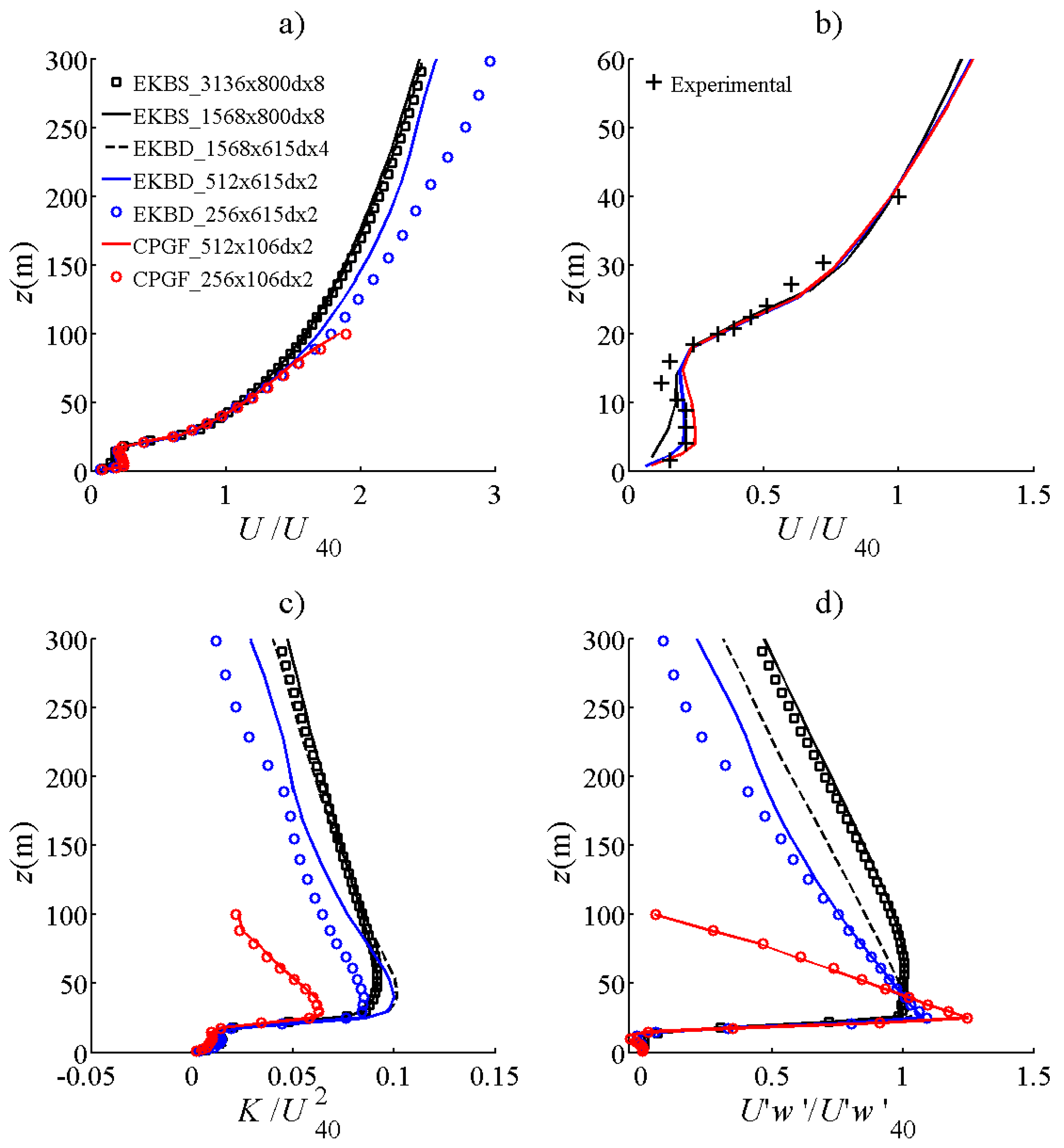
Figure 3 shows profiles of normalized wind statistics, as well as the reference experimental wind profile, for simulations done with various grids using EKBS, EKBD, and CPGF (canopy Can1). Streamwise velocities U ( = u 2 + v 2 ), turbulent kinetic energy K and momentum flux U ′w′ are, respectively, normalized by U 40 , U 40 2 and U w 40 , where U 40 and U w 40 are the streamwise velocity and momentum flux at 40 m. This reference height was selected because it is high enough to undergo a limited influence of the canopy (more than 2h), while remaining theoretically measurable from the ground. The profiles show similar shapes and characteristic features. For example, all of the wind profiles have an inflection below the canopy and are quasi logarithmic above it. The turbulent kinetic energy and the momentum flux both show a maximum above canopy height. In particular, the turbulent statistics of the simulation done on the largest domain (EKBS_3136x3136dx8, in black squares) are almost identical to EKBS_1568x800dx8 (black line), suggesting that a domain of 1568m is long enough for this type of runs and that the EKBS_1568x800dx8 is relevant as a reference boundary-layer simulation. The vertical resolution affects profile quality below the canopy top (Figure 3b), the coarser resolution (1/3rd of the canopy height, black line) leading to a much smoother profile than in the experiment, whereas there is good agreement below the canopy top in the case when the vertical resolution is close to 1/10th of the canopy height (simulations corresponding to domain heights of 615 and 106 m, respectively, in blue and red). The biggest differences occur when the domain size is reduced below 256 m: Streamwise velocity profiles for domain lengths of 256 m (EKBD_256x615dx2, blue circle) and heights of 106 m (CPGFs, red line and circles) diverge from the other profiles above 80 m. Moreover, the turbulent kinetic energy and momentum flux begin to fall off at lower heights when the domain length is smaller than 512 m. The decline starts at the lowest heights and is the strongest on 106-m high domains. These results indicate that the wildfire-precursor simulation (EKBD_512x512x615dx2) and EKBD_1568x615dx4 are the only two simulations that exhibit similar features to the boundary-layer simulation far above the canopy, as well as a profile below the canopy which is consistent with observations.
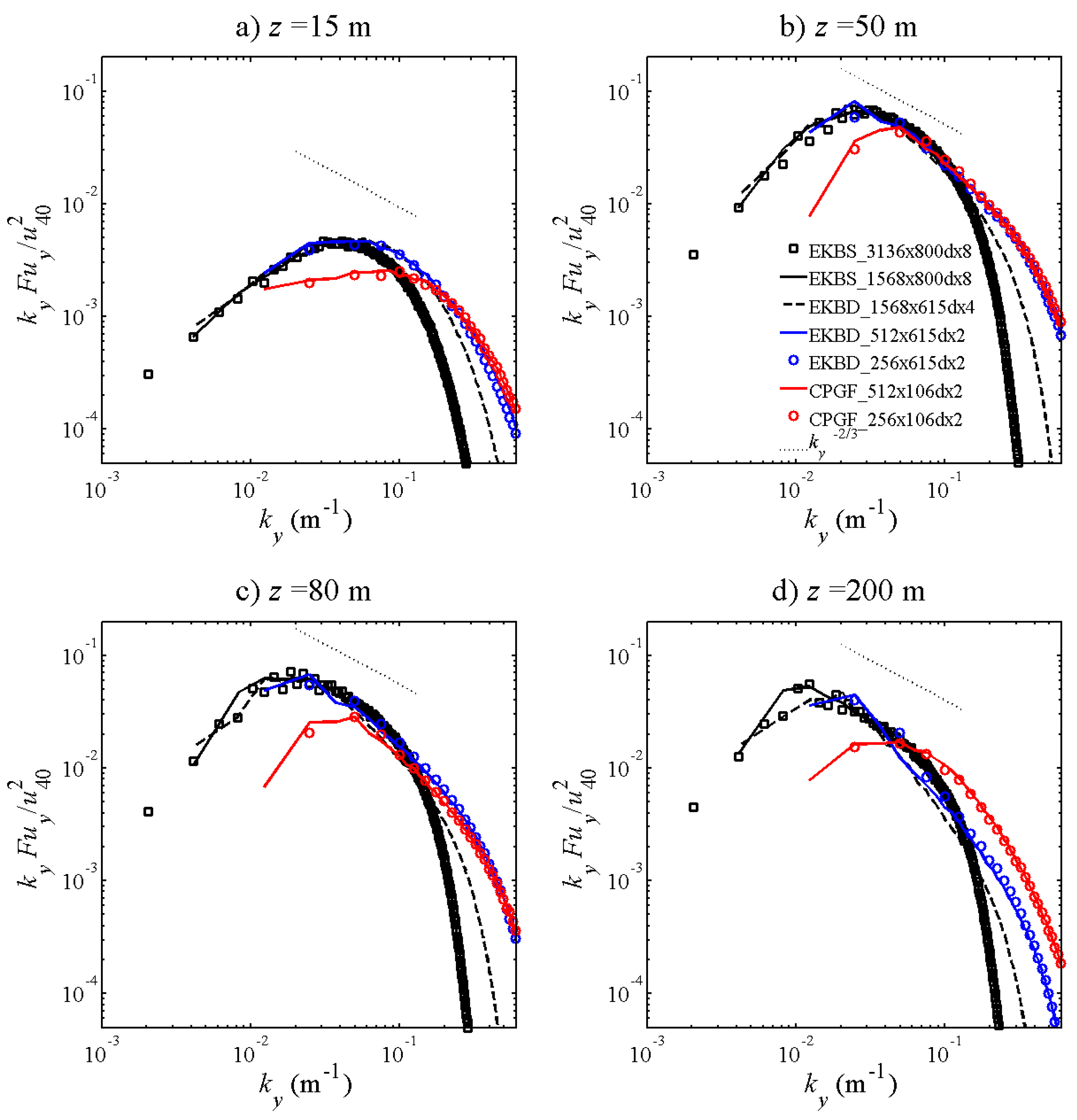
Figure 4 shows the spectral analysis of the u-velocity component at several heights. The portion of the spectra with −2/3 slope is characteristic of a fully-developed turbulent flow. At the highest frequency (turbulent structures smaller than ≈8dx), the energy fell off steeper than −2/3, due to numerical dissipation [41]. This fall-off appears at a much higher frequency for the simulations using the highest resolution (dx = 2 m; fine vertical resolution, in blue or red) than for the simulation with dx = 8 m (black squares and line), the simulation with dx = 4 m being in between (black-dashed line). This confirms that a significant part of fine-scale turbulence is lost when the coarse resolution is used.
The black-line spectra and black-dashed spectra can, thus, be taken as a reference for the frequencies lower than 0.131 m−1 (turbulent structures smaller than 6dx = 48) and for frequencies lower than 0.262 m−1 (6dx = 24), respectively. The spectral energy of EKBD_512x615dx2 (blue line) is almost identical to those of the larger EKB domains at these wavelengths, suggesting that the corresponding domain size and resolution are a good compromise between structure accuracy and computational cost. The CPGF simulations with the 106 m height domain (in red) clearly underestimate the spectral density of the largest structures, which explains why the turbulent kinetic energy profiles are much lower for these simulations than for the others, especially above the canopy (Figure 3).
To conclude this subsection, EKBS_1568x800dx8 can be used as a reference boundary-layer simulation. EKBD_512x615dx2 performs better below the canopy and explicitly simulates smaller turbulent structure, without large bias on the energy of the largest structures. Considering the trade-off between domain size and resolution, it appears as an appropriate reference for wildfire-precursor simulation. In the next subsections, the PGF and CPGF simulations are systematically compared to these two reference simulations.

4.2. Evaluation of PGF-Boundary-Layer Simulations (1568 m × 1568 m × 800 m)

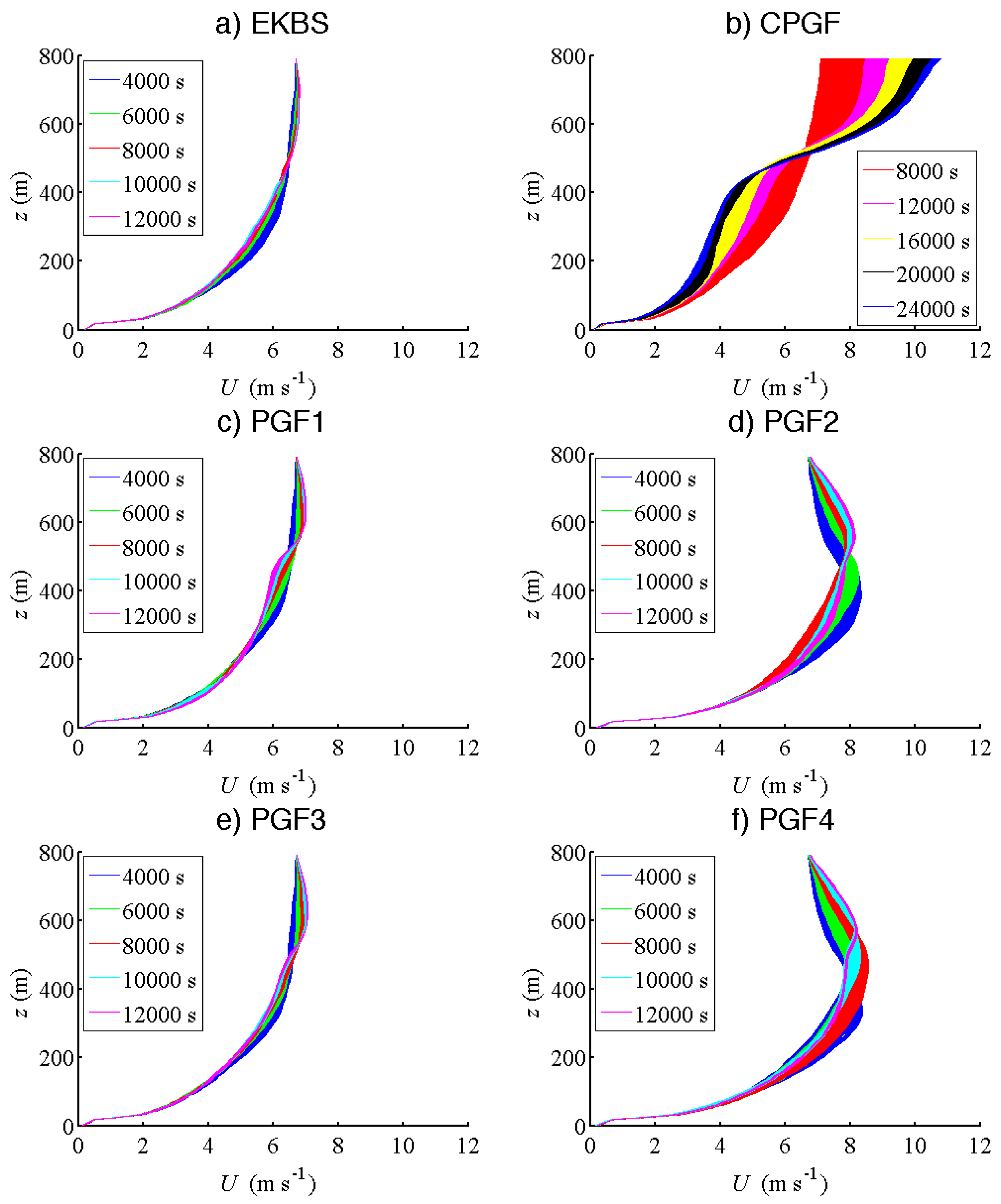
In this subsection, the simulations using PGF and CPGF are compared to the reference boundary-layer simulation (EKBS_1568x800dx8). For simplicity, we use only the prefix of the simulation names, since the same grid (1568 m × 1568 m × 800 m, with dx = 8 m, d z ¯ = 10 m and 0.4 stretching factor over the vertical) is used in these simulations. Figure 5 represents the temporal evolution of vertical profiles of horizontally-averaged velocities. For each simulation, a plot shows a sequence of instantaneous profiles taken every 200 s. In blue are plotted the profiles obtained between 0 and 4000 s, in green, between 4000 and 6000 s, etc. After 4000 s of simulated time, the evolution of the EKBS wind profile slows, and changes are limited in magnitude. Thus, we can consider that the stable Ekman balance is reached at this time (Figure 5a). When the constant pressure gradient is used (CPGF, Figure 5b), the wind velocity below the capping inversion slowly declines, and the profile converges toward an S-shape profile (below 500 m). The decline in the lower elevations is counterbalanced by an acceleration in the upper elevations, to keep the mass flow constant. PGF1 and PGF3 profiles (Figure 5c,e) both converge quickly toward profiles similar in shape to the EKBS profile. PGF2 and PGF4 (Figure 5d,f) converge slower, and profiles are slightly different. However, the mean wind velocities at zref = 40 m ( U 40 ) of PGF2 and PGF4 are very close to the target velocity of 3 m s−1 (Table 5). For the other simulations (including EKBS), U 40 is in general much lower than the target wind speed (Table 5), illustrating that the geostrophic wind value chosen for this computation (6.7 m s−1, estimated using empirical profiles described in Appendix A), is too low to reach the target velocity of 3 m s−1 at 40 m. This result illustrates that reaching a target velocity close to the canopy from a specified geostrophic wind is challenging.
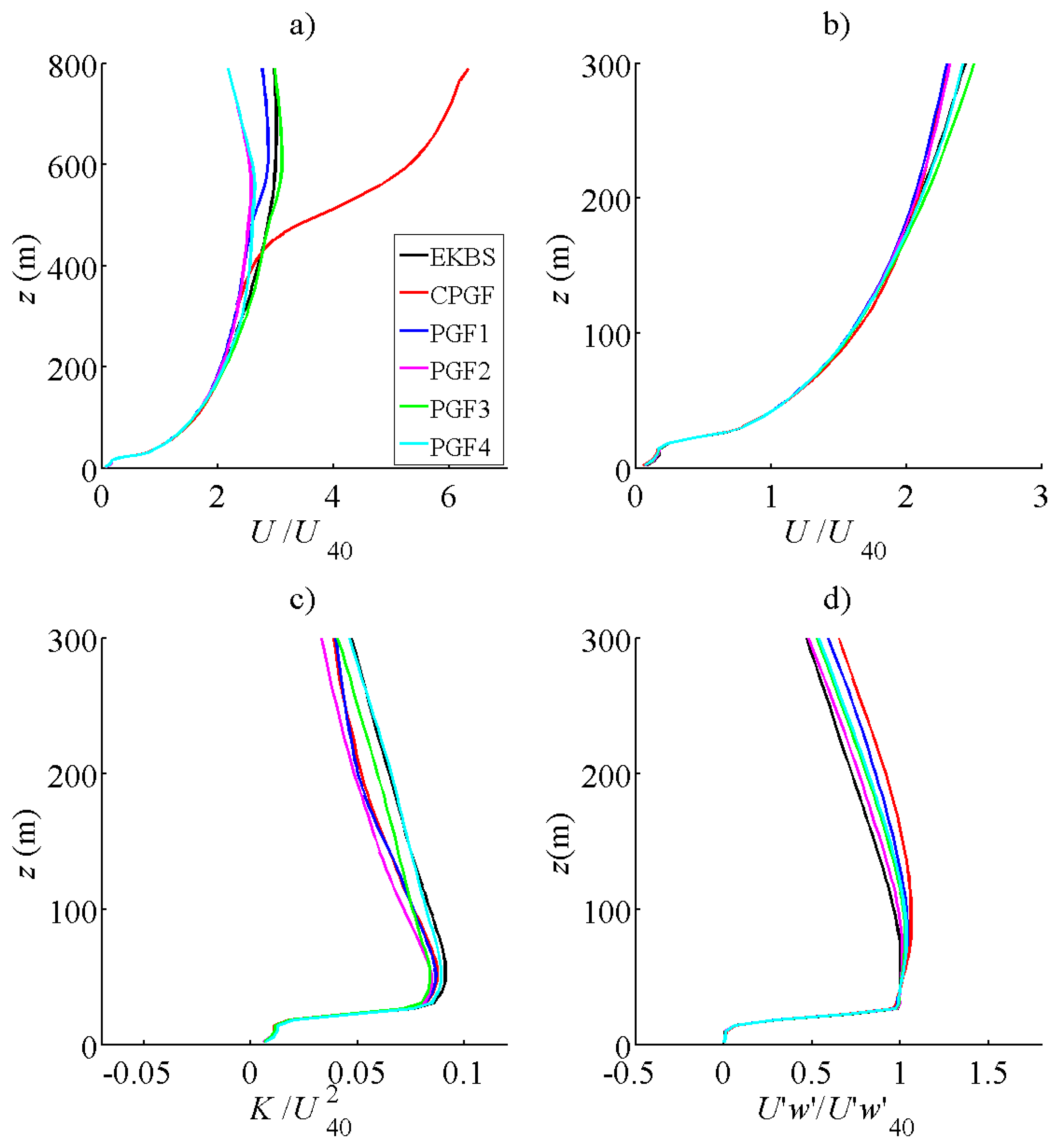
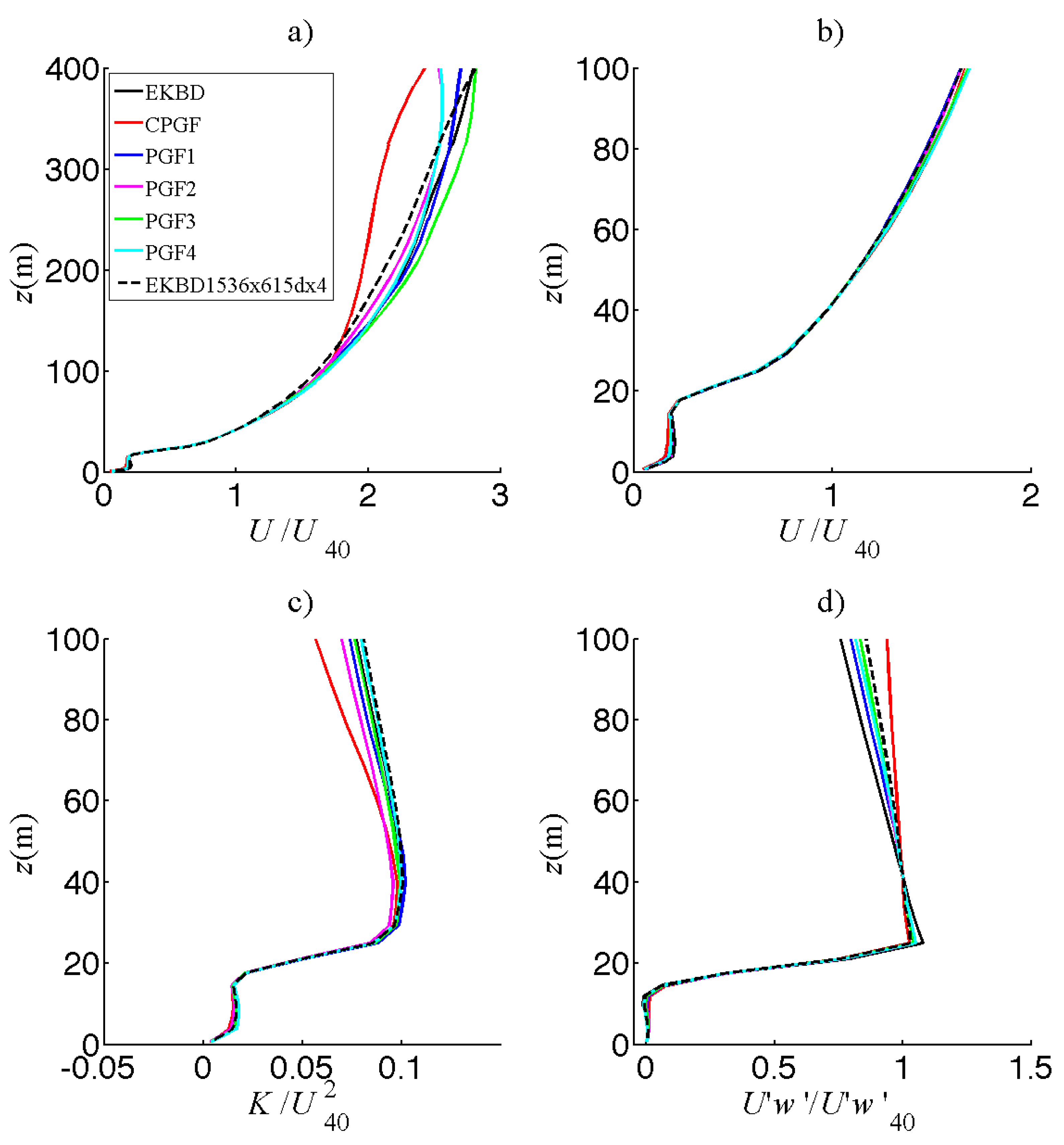
Figure 6 shows normalized turbulent statistics, averaged on both space and time (7200–10,800 s). Turbulent statistics have the same features as those presented for EKB simulations in Figure 3, except CPGF, which exhibits an S-shape velocity profile below the capping inversion (Figure 6a). PGF simulation are close together, generally similar to EKBS. The turbulent kinetic energy of PGF1 and PGF2 are slightly underestimated above the canopy (Figure 6c), whereas momentum fluxes are overestimated (Figure 6d). The PGF3 and PGF4 are the most similar to EKBS, even if the PGF4 wind profile exhibits differences in its upper part for the reason mentioned above (Figure 6a). The major benefit of PGF2 and PGF4 is to reach the target wind speed with turbulent statistics very similar to those of the reference case below 300 m and a normalized wind profile only slightly different above 300 m (Table 5), whereas the other simulations (including EKB) show much lower U 40 .
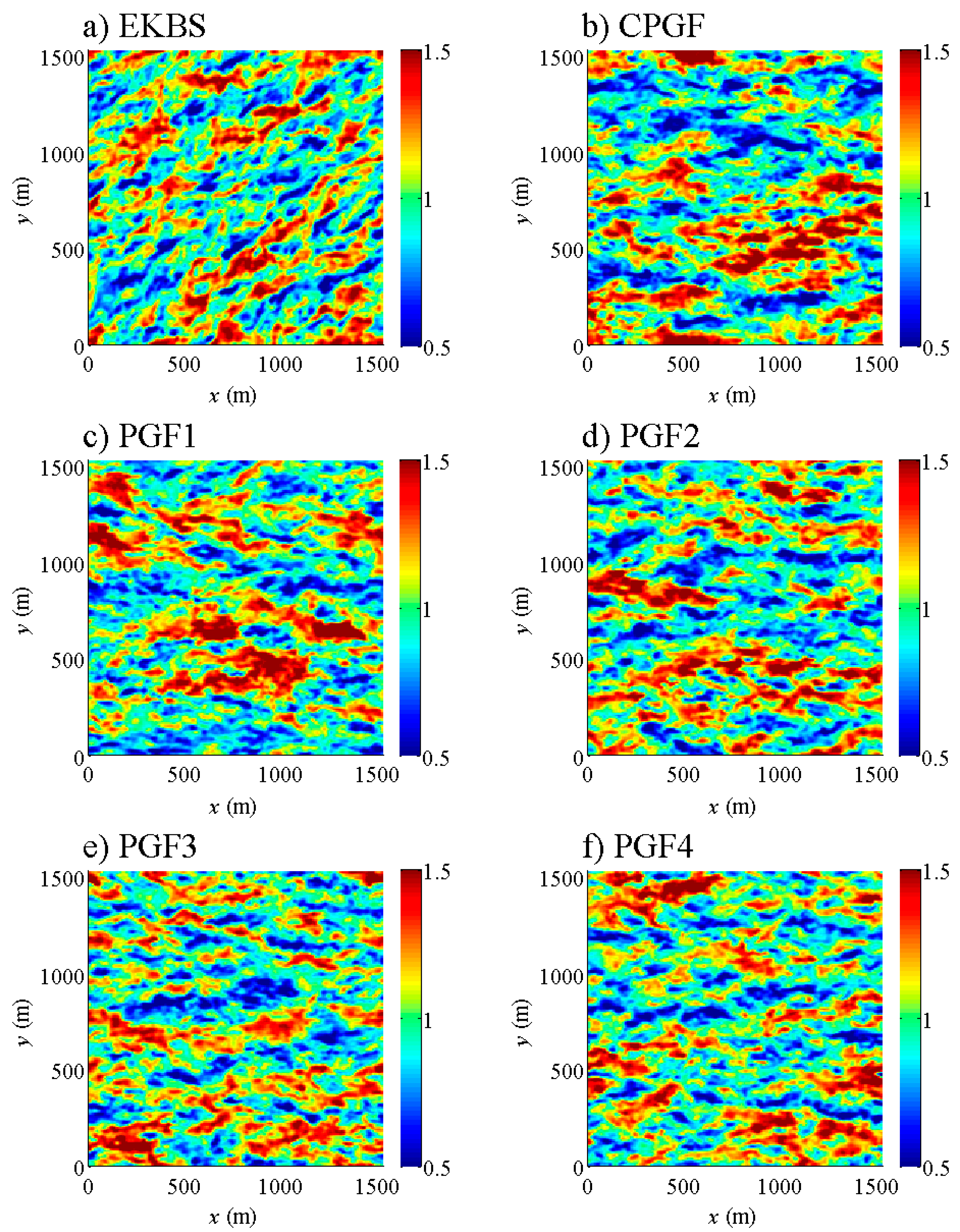
Figure 7 presents instantaneous contours of horizontal wind velocity on a horizontal plane at z = 56 m. Elongated structures of high-speed and low-speed are evident. For EKBS, the structures are tilted, due to the Coriolis force (Figure 7a), whereas they are aligned with the x-axis for the other simulations (Figure 7b–f). This observation of streaky structures (related to vertical motions) is consistent with other LES studies listed in the introduction. Beyond the tilt angle, the structures obtained for the other simulations are visually similar to those of EKB.
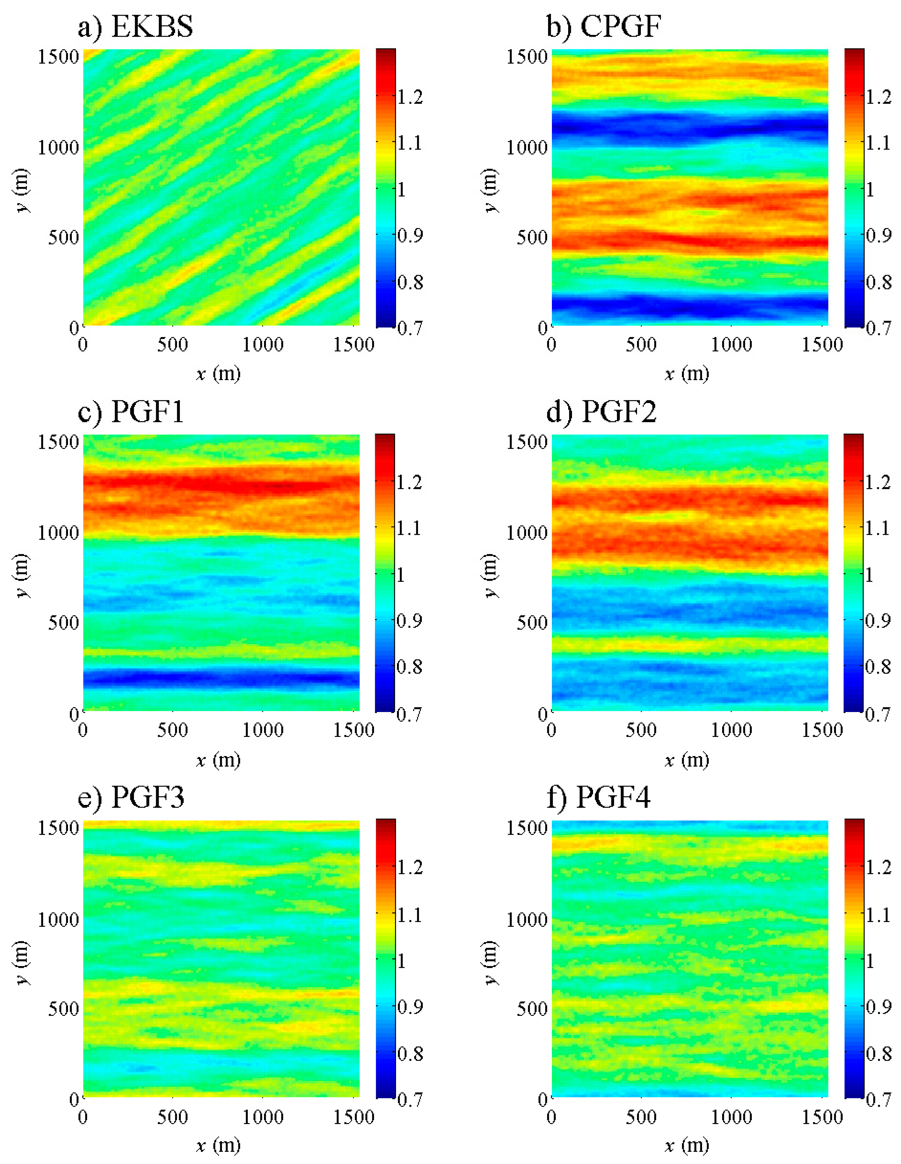
When averaged over one hour (Figure 8), the plots reveal that the larger structures tend to be maintained over time. All simulations, including EKBS, produce a streaky structure with alternating slow and fast regions. The reference simulation (EKBS, Figure 8a) has several streaks of limited magnitude (about 10% of the mean value). Among the other cases, CPGF, PGF1, and PGF2 (Figure 8b–d) present a streaky structure dissimilar to the EKBS, with two locked streaks of strong magnitude (more than 30% of the mean value), showing patterns similar to those observed by Reference [2]. Due to the pressure-gradient forcing that varies in the crosswind direction, PGF3 and PGF4 present several streaky structures (Figure 8e,f), which are visually similar in size and magnitude to those of EKBS (aside from the rotation of the wind field).
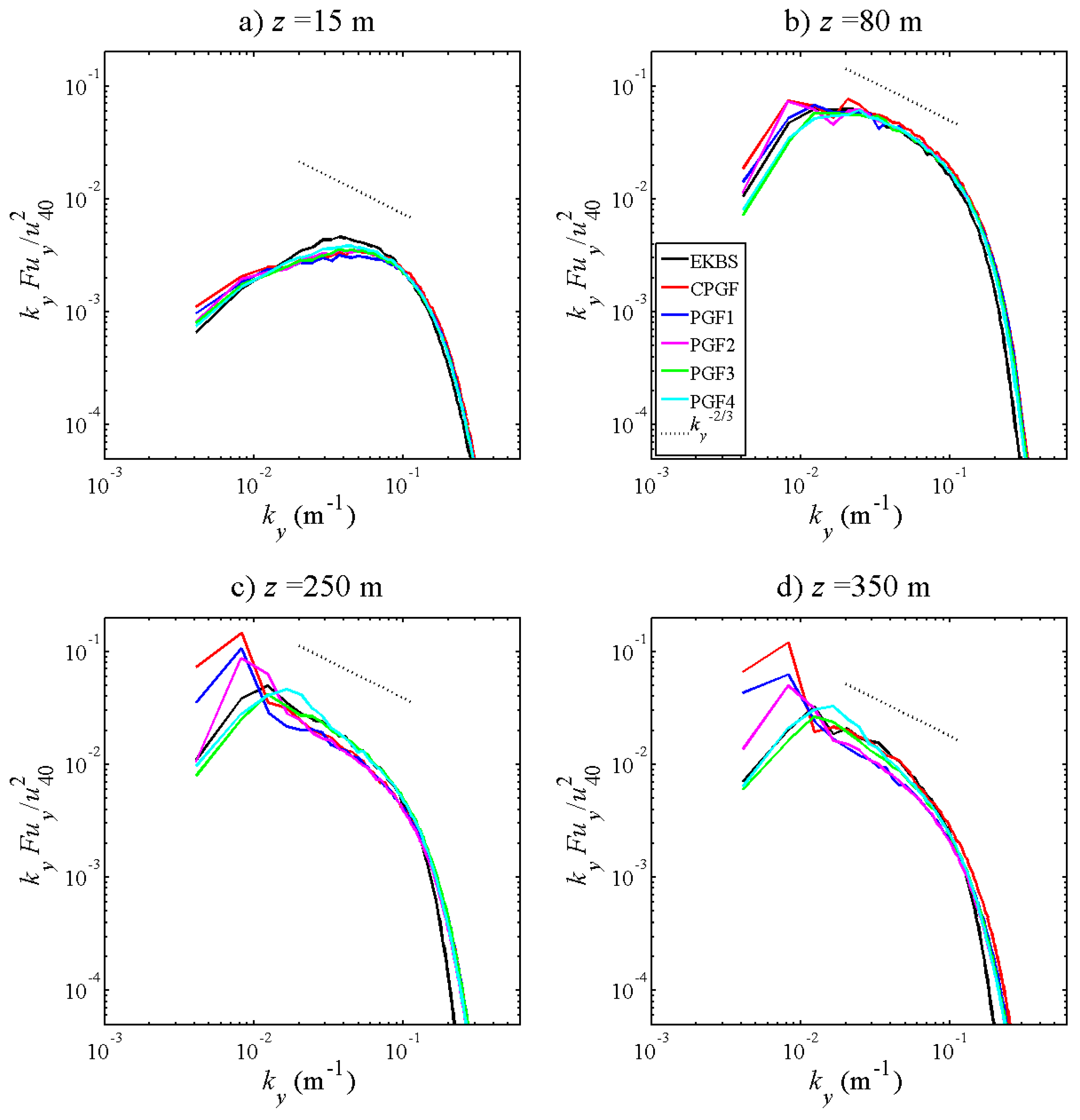
Figure 9 shows the spectral analysis of the u-velocity at various heights. The PGF and CPGF simulations are, in general, similar to EKBS for the highest wavenumbers (greater than 0.021, which is 300 m). However, CPGF, PGF1, and PGF2 show much higher spectral density at the lowest frequencies. This is especially true in the upper part of the domain, where the spectral density increases by a factor of two or more compared to EKBS at the frequency corresponding to mid domain extent (frequency of 0.0082, Figure 9c,d). This is explained by the magnitude of the two locked streaks, especially visible in Figure 8b for CPGF. PGF3 and PGF4 show the most similar turbulent spectra to EKBD, thanks to the local control in horizontal planes by the laterally-heterogeneous pressure gradient.

4.3. Evaluation of PGF-Wildfire-Precursor Simulations (512 m × 512 m × 615 m)

In this subsection, we compare simulations with PGF and CPGF, forcing to the results obtained with EKB for the wildfire-precursor simulation. For simplicity, we use only the prefix of simulation name, since the same grid (512 m × 512 m × 615 m, with dx = 2 m, d z ¯   = 15 m and 0.1 stretching factor over the vertical) is used for the simulations. The only exception is EKBD1536x615dx4, plotted in black-dashed lines to ease comparison with boundary-layer features, to evaluate the ability of this wildfire-precursor simulation to render the large boundary-layer features (see Section 4.1 and Section 4.2 for details). Figure 10 shows normalized turbulent statistics below 400 and 100 m. As for boundary-layer simulations, all canopy-flow simulations show the expected features. EKBD and EKBD1536x615dx4 are very close, showing that the resolution and domain size does not significantly affect the statistics using EKB. The CPGF is characterized by the S-shape profile (lower below 400 m is visible in Figure 10a) and a nearly constant momentum flux above the canopy. This simulation is the most dissimilar to EKB, highlighting the limitations of CPGF in the context of wildfire-precursor simulations.
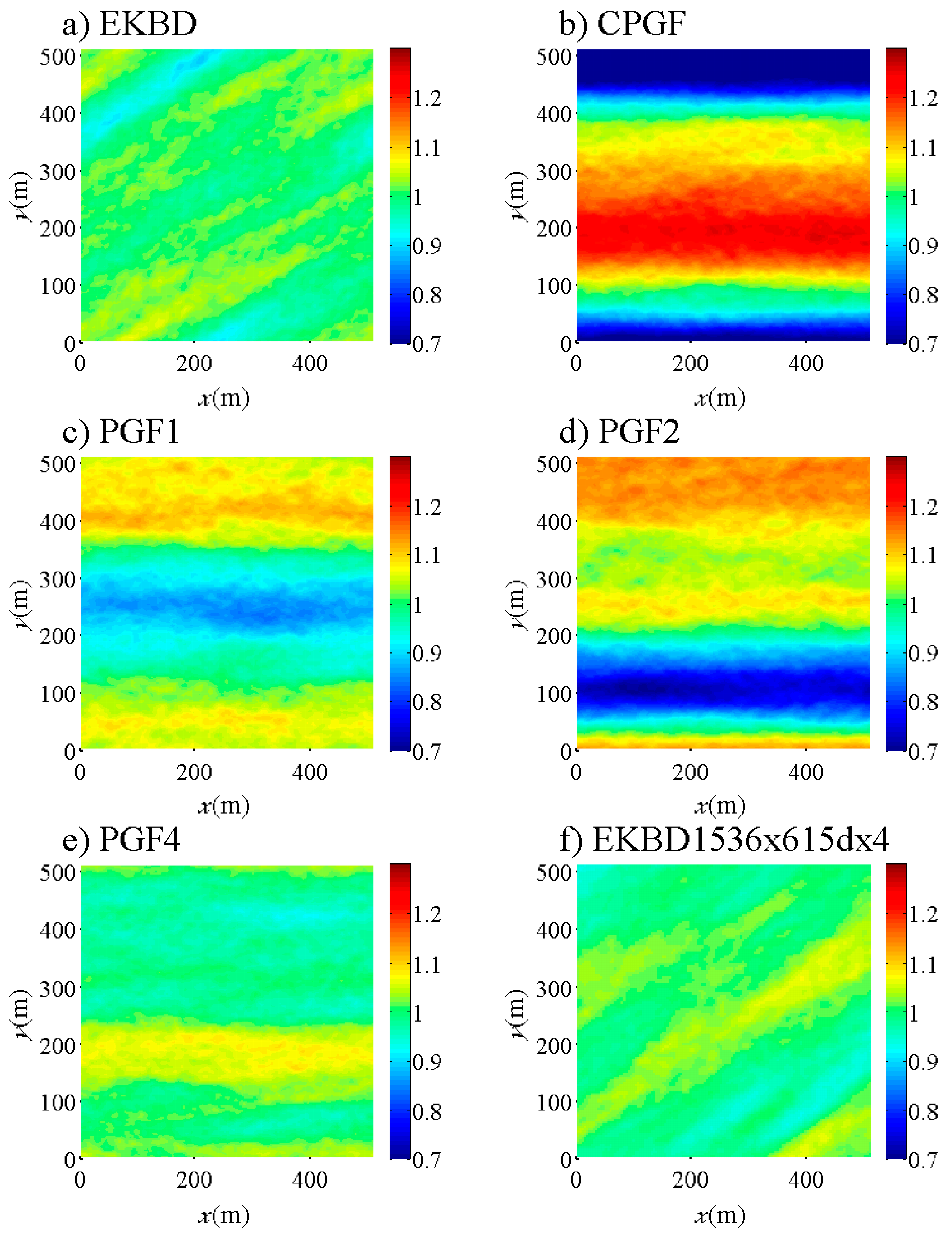
Figure 11 reveals the streaky structures occurring when canopy flow simulations are averaged over one hour. As in Figure 8, the plots reveal that the magnitude of the streaky structure is much greater for CPGF, PGF1, and PGF2 than for the EKBD. Figure 11f presents the streaky structure for the EKBD1536x615dx4, with a zoom on a 512 m × 512 m subdomain to allow comparison with canopy-flow simulations. Figure 11a,f visually show that the structures obtained on the 512-m domain are similar to those of the 1536-m domain. As already observed for boundary-layer simulations, PGF4 (and PGF3 not shown) show a similar magnitude of streaky structures as EKB (Figure 11e).
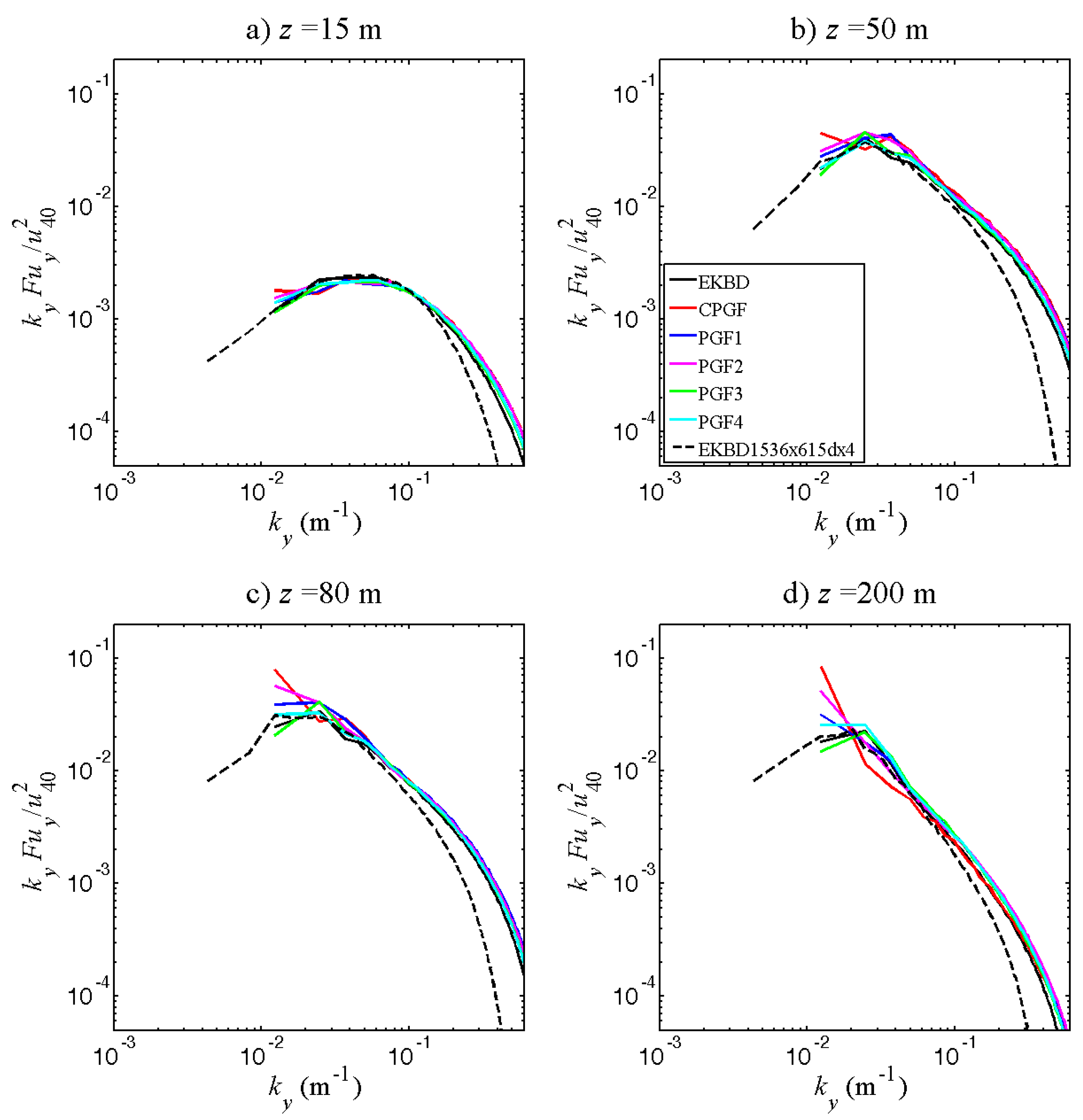
Figure 12 shows the spectral analysis for the u-velocity at various heights. As already observed in Figure 4, EKBD and EKBD1536x615dx4 are similar, except for the highest frequencies, due to the coarser spatial resolution of EKBD1536x615dx4. The comparisons between PGFs, CPGF, and EKB for canopy flows leads to the same conclusion as for the boundary-layer simulations. CPGF shows the highest spectral densities for the largest structures, whereas PGF3 and PGF4 are the most similar to EKB. PGF1 and PGF2 rank between them.

5. Discussion

The vertical profiles of turbulent statistics and turbulent spectra, shown in the present manuscript, enable comparison of major aspects of EKB, CPGF, and PGF and the influences of domain size and resolution when used to simulate wind flows within and above forest canopy for applied studies. The comparison of the different coherent structures is not as detailed as what could be achieved using multivariate methods of statistical analysis, such as the proper orthogonal decomposition (POD). However, in this context, they enable us to (1) clearly demonstrate some limits of EKB and CPGF in this context, (2) examine to which degree the proposed method solves these identified limits, (3) illustrate the consequences of domain size and resolution on main features. These points are developed in the following subsections.

5.1. Limitations of CPGF and EKB Approaches for Flow Simulations within and above Canopies

Our simulations show that the S-shape profile, already observed with CPGF by Reference [42], occurs in configurations when near-ground drag elements are resolved. Hence, simulated flows with CPGF differs from the expected features of the upper part of the atmospheric boundary layer. Moreover, the magnitude and locking of the streaky structure are clearly stronger with CPGF than with EKB simulations, which can be taken as a reference to idealized atmospheric flow. This finding is in agreement with the results of Reference [29], who identify a stabilizing role of Coriolis force on streamwise coherent structures. As explained in Section 2, CPGF only induces a convergence of the spatially-averaged profile, whereas EKB is a stable equilibrium that has a damping effect on persistent lateral heterogeneities. This different nature of the two forcing types explains why streaks are locked when using CPGF, because they can persist and grow over time with a spatially-constant forcing, while they are damped by the EKB.
The EKB enables a rapid convergence of the flow, satisfactory turbulent statistics close to the canopy when the resolution is fine enough, and evolving streaky structures. However, the magnitude of the wind velocity in the canopy neighborhood is only controlled by the geostrophic wind value, which is not practical when working on canopy flows or trying to establish a turbulent profile that matches observations, such as those measured from towers. Even when realistic initial profiles are used, the convergence in the lower part of the canopy can be far from the expected value (2.24 m s−1 instead of 3 m s−1), which is a drawback for several applications, particularly for wildfire-precursor simulations. This limitation can eventually be solved by trial and error methods at the price of the user and computational times. However, this process is considerably complicated by the angle of rotation of the wind direction, which also varies with geostrophic wind magnitude, elevation reference, and vegetation type. In the simulations of the present paper, this rotation varies between 25 and 40°. This rotation complicates modeling applications even more, as the direction can vary abruptly near the canopy top. Indeed, wind velocities are so small below the canopy, that the Coriolis and drag forces become negligible compared to the mesoscale pressure gradient [43]. As a consequence, the rotation between the top and the bottom of the canopy can be important. Although neglected in most canopy-flow or wildfire simulations, such a rotation has been reported in deep and dense canopies [43], and observed in simulations [44], in which the wind direction tends to align with the mesoscale pressure gradient below the canopy, i.e., orthogonal to the geostrophic wind [9]. At coarser scales, simulations over-idealized topography become more complex in the presence of this rotation. Even if the EKB probably leads to more realistic flows within and above canopies than CPGF, this physical framework should not be seen as a fully realistic scenario, since it relies on some strong assumptions, such as the mesoscale pressure gradient taken constantly over the domain. In practice, it is not necessarily constant neither over the vertical extent of the domain, nor along the distance traveled by the flow in a periodic simulation of several hours. Considering how sensitive the rotation is to vegetation and wind velocity, it is likely that its direction strongly depends on local variations of the pressure gradient, which could lead to either overestimation or underestimation of the rotation near the canopy. As an example, the authors of Reference [9] noticed that the rotation that they observed in their simulations was not present in the field dataset. Another point is the fact that it is unclear to the authors if these steep changes in direction in the lower part of the domain are consistent with the use of periodic boundary conditions when vegetation is heterogeneous. Indeed, the wind direction at a given height can be significantly different inside a forest and in a clearing, for example, leading to a confusing situation. We think that further investigations are required to evaluate the consequences of this constant mesoscale-pressure-gradient assumption in EKB scenarios. For these reasons, EKB forcing has never been used in wildfire or wind turbine precursor computations to the best of our knowledge.

5.2. Applicability of PGF-Methods to Idealized Boundary-Layer, Canopy-Flow, and Wildfire-Precursor Simulations

The PGF methods developed aim at providing a pressure-gradient forcing that avoids the complexity and uncertainty induced by the spiraling of the EKB, but which (1) is based on a more realistic pressure profile than the CPGF, (2) does not lead to locked streaky structures as CPGF, and (3) enables the prescription of a target velocity vector.
PGF1 used a more realistic vertical pressure gradient forcing than CPGF, which is derived from the EKB and enables to avoid the S-shape profile. PGF2 and PGF4 enable the control of velocity magnitude and direction. PGF1 and PGF2 have the same drawback as CPGF in terms of production and locking of strong streaks (compared to the EKB), since the local forcing does not possess the damping features required to suppress the intensification of locked streaks. Therefore, their application should be limited to very long domains, in which locking is limited. For example, Reference [45] showed that very large streamwise-elongated coherent structures, with a length of the order of tens of the boundary-layer thickness, contribute significantly to an atmospheric boundary-layer simulated with CPGF. PGF3 and PGF4 include a streak-damping or streak-blending mechanism based on a pressure gradient that is not uniform in the crosswise direction, to limit the magnitude of streaky structures and their trend to get locked. A valuable alternative to PGF3 and PGF4 could be to combine PGF1 or PGF2 with shifted boundary conditions, which can mitigate streak locking [36]. This will be tested in the future. We would like to point, however, that the stabilization mechanism of PGF3 and PGF4 mimics the combination of the Coriolis force and the mesoscale pressure gradient, that acts to speed up or speed down the flow that would be locally slower or faster than the equilibrium value at a given height, contrary to the shifted boundary condition that simply acts as a numerical solution to artificially increase domain length. In the present study, we found that the streaky structure over one hour is similar to the one of the EKB. Also, the turbulence spectra are very similar for PGF and EKB (except for the lowest wavenumbers), suggesting that the contribution of the Coriolis force in the turbulence cascade is probably limited. As a consequence, the wind flows developed with PGF3 and PGF4 methods appear as a non-spiraling version of the canonical EKB simulation. In scenarios in which a rotation with height is desired, but expected to be controlled (for example, prescribing a given angle at a reference height), PGF methods can be adapted to force such a rotation (following Ekman spiral or any other equations providing the desired spiraling).
In our PGF approaches (as for CPGF), a value must be given to the parameter Δ t , the period at which an update of pressure gradient forcing is calculated. In the simulations presented here, we choose Δ t = 200 s as stated in Section 2. This value was taken because periodic simulations with no pressure gradient led to a decay rate of integrated momentum, which is typically about 5% every 200 s in the lower part of the domain (not shown); therefore, 200 s can be seen as a relevant characteristic time for the action of the large-scale pressure gradient on the mean flow. When elaborating the method, we also tested values 100 and 400 s and found the results to be relatively insensitive within this range of parameter values. However, some high-frequency oscillations of the wind flow with time appear in the lower part of the domain when Δ t is too small ( ~ 10 s), because F is modified much faster than the time required for a change in mean flow. In contrast, when choosing Δ t too large ( ~ 2000 s), some slow oscillations of the integrated momentum occur. The value of 200 s was chosen for all simulations presented here, showing that PGF is relatively insensitive to domain size or canopy type.

5.3. Comparison of PGF Wildfire-Precursor Simulations to Observations and Application to Heterogeneous Scenarios

Several authors have already observed that turbulence statistics obtained with LES without pressure gradient, or forced with CPGF or EKB [4,5,6,9,33,46] are close to empirical data. We obtain good agreement with PGF1–4 for experimental datasets corresponding to canopies Can1 to Can4, as illustrated with PGF4 as an example in Appendix C. This shows that PGF methods do not degrade the predictions near the canopy, which is not surprising as corresponding features are shear-dominated.
Canopies Can2 and Can4 corresponds to heterogeneous landscapes (clearing to forest transition). Using PGF4 as done in Appendix C remains relevant because the vegetation distribution is constant in the crosswise direction. More generally, forcing the integrated momentum for the streamwise direction only makes sense when the integral of leaf-area density (LAD) in the streamwise direction is nearly uniform along the crosswise direction. Potential issues that may arise from heterogeneous vegetation along the crosswise direction are not specific to PGF and concern any simulations using periodic boundary conditions, whatever the type of forcing. For example, periodic boundary conditions are not appropriate to simulate wind flows blowing parallel to a forest edge, because the mass flow cannot be infinitely faster along some streamwise path (clearing) than others (forest) without breaking the hypothesis of a constant mesoscale pressure gradient in the domain. The challenge associated with domains containing large-scale heterogeneity, can be solved by using the nested domains [47,48]. With this technique, an ambient wind flow over a much larger domain with homogenized vegetation and topography (or with heterogeneities that are small compared to domain extents) can be simulated using PGF4. The results of this simulation can then be used as inlet and outlet precursors on a more refined domain with substantial heterogeneous vegetation or topography, as done by Reference [49]. Another consideration for the application of PGF to heterogeneous landscapes (such as canopy Can2 and Can4) is the question of where the target velocity is defined. More specifically, field data are often collected in an open area. To account for that, the calculation of the integrated momentum presented in Table 1 can be limited to an appropriate subdomain, for instance, the clearing area in which the collected data is representative, as done by Reference [49].

5.4. Domain Size and Resolution of Canopy-Flow LES

LES have been applied to a wide range of domain sizes and resolutions, depending on the objectives of the simulations. Our sensitivity study demonstrates that the choice of the set-up is critical regarding the features of interest. The authors of Reference [45] used LES to simulate Very-Large-Scale-Motions in 25-km domains and showed that 27% of the energy is available in scales larger than 10 km. However, the resolution of such simulations (50 m) is obviously not well-suited to reproduce canopy-flow statistics and wildfire precursors for detailed physics-based models, such as HIGRAD-FIRETEC. In particular, a grid finer than ~1/3 of canopy height is required to reproduce wind profiles inside canopies, contrary to ~1/10th canopy height resolution, for which turbulent structures of size in the order of canopy height can be resolved.
These fine-scale turbulent structures are of great importance in the context of canopy functioning, seed or pollen transport, windthrow, or wildland fires. For these specific applications and for a limited time of simulation (e.g., one hour), it is probably more important to accurately simulate these small structures than the largest ones, which evolve slowly over a short time line. On the other hand, our sensitivity analysis shows that the simulations done with 106-m domain heights fail to simulate structures larger than canopy height, in particular, the turbulent kinetic energy and the momentum flux above the canopy. These simulated configurations proved very helpful to understand the details of shear dominated canopy flow, but larger domains are probably required for applications potentially affected by slightly larger structures, such as wildfires.
When the focus shifts from the surface and canopy winds to those above the upper part of the plume of a large or intense wildfire, much larger horizontal domains must be used, and neglecting Coriolis force or assuming a constant mesoscale pressure gradient is likely, not satisfactory. Instead of running the model under idealized scenarios with periodic boundary conditions, it is better to prescribe ambient variables (potential temperature, pressure, wind velocities) modeled with mesoscale models [19].

6. Conclusions

This paper’s main objective was to present approaches developed to capture the effects of pressure-gradient forcing for canopy-flow LES simulations, such as those performed with HIGRAD/FIRETEC or a broader class of LES boundary-layer simulations. In such simulations, the focus resides in the near-surface flow features, which is especially the case of wildfires. These approaches (PGFs) overcome some drawbacks of existing forcing (Ekman balance EKB and constant pressure gradient forcing CPGF), including the lack of control on wind speed and direction close to the ground. Our analysis demonstrates that the use of CPGF with high domain systematically results in unrealistic locked streaky structures, due to the lack of local forcing to damp them and the short domain horizontal extents. Also, turbulent statistics and spectra obtained with CPGF applied in a vertically-short domain—which is typical of CPGF usage—are fairly different from those obtained with the more realistic Ekman balance and a boundary-layer simulation set up. In particular, such simulations in small domains fail to adequately simulate larger structures. On the other hand, the simulations over large domains with low resolution fail to explicitly calculate turbulent structures on the order of canopy height or to reproduce the wind profile below the canopy.
The typical grid used for wildfire-precursor simulation forced with PGF with HIGRAD/FIRETEC is a compromise between computational cost and realism of simulated wind field. Regarding the different PGF methods, PGF2 and PGF4 enable mechanisms to control the velocity magnitude at a given height, whereas PGF3 and PGF4 are designed to damp the development of streaky structures and produce lateral flow heterogeneities, similar to those of EKB (beyond the rotation due to Coriolis)—at least in the lower part of the domain. Comparison with experimental data collected near the canopy showed that PGF methods perform similarly in terms of turbulence statistics to existing approaches and studies. PGF4 can be used directly when vegetation and topography are statistically homogeneous in the crosswind direction. When it is not the case, it can be used on a homogenized landscape to generate precursors for the proper heterogeneous domain.

Author Contributions

Conceptualization, F.P., J.-L.D. and R.R.L.; methodology, validation, formal analysis, writing—original draft preparation, F.P.; writing—review and editing, all authors. All authors have read and agreed to the published version of the manuscript.

Funding

This research received no external funding.

Acknowledgments

We would like to thank Sylvain Dupont from INRA and two anonymous reviewers of a former version of this work, who provided very useful comments, which significantly improved this manuscript. The Los Alamos National Laboratory Institutional Computing Program provided the critical computing resources for this work.

Conflicts of Interest

The authors declare no conflict of interest.

Appendix A. Initial Empirical Wind Profile

The initial wind profile for the HIGRAD/FIRETEC simulations is derived from existing empirical-based functions. This formulation requires vegetation characteristics to compute a mean leaf area index (LAI) for the stand:
L A I = 1 2 l x l y 0 l x , l y , h ρ ρ w o o d σ d x d y d z ,
where lx and lx are the lengths of the domain along the x and y axes, and h the maximum height of the fuel bed or canopy. ρ , ρ w o o d and σ are the bulk density, wood density and particle surface area to volume ratio of the fuel, respectively. The ρ / ρ w o o d ratio is the local volume fraction of the fuel. The shape of an empirically-based velocity profile u ^ ( z ) presented by References [33,50] can be computed in the following piecewise manner:
for   z h ,   u ^ ( z ) = exp ( c 4 ( 1 z h ) ) ,
for   z 2 h ,   u ^ ( z ) = c 1 0.41 ln ( z h + c 2 1 c 3 ) ,
When z is between h and 2h, a cubic polynomial regression is made between u ^ ( h ) and u ^ ( 2 h ) .
c 1 = min ( 0.003 + 0.15 L A I , 0.3 ) ,
c 2 = 1 exp ( 7.5 L A I ) 7.5 L A I ,
c 3 = c 2 exp ( 0.41 c 1 0.19 ) ,
c4 = max(min(0.5LAI + 1.2, 3.2),1.7),
Given horizontal velocity components, ( u r e f , v r e f ) , at a reference height z r e f , the magnitude of the initial wind flow is determined as a function of height, z, as follows:
u i n i t ( x , y , z ) = u r e f u ^ ( z ) u ^ ( z r e f ) ,
v i n i t ( x , y , z ) = v r e f u ^ ( z ) u ^ ( z r e f ) ,
where the upper script init indicates the initial value. For the simulations of the present study, the ambient wind velocity in the x-direction, u r e f at z r e f = 40 m above ground level is 3 m s−1 and v r e f = 0 except for EKBS and EKBD, where the Ekman spiral angle is applied to the initial profile to speed up the convergence to the EKB.
This empirical profile can also be used to get a crude estimate of the velocities in the damping layer at the top of the domain if one is used.

Appendix B. Implementation of PGF4 When the Flow Is Not Aligned with a Domain Axis
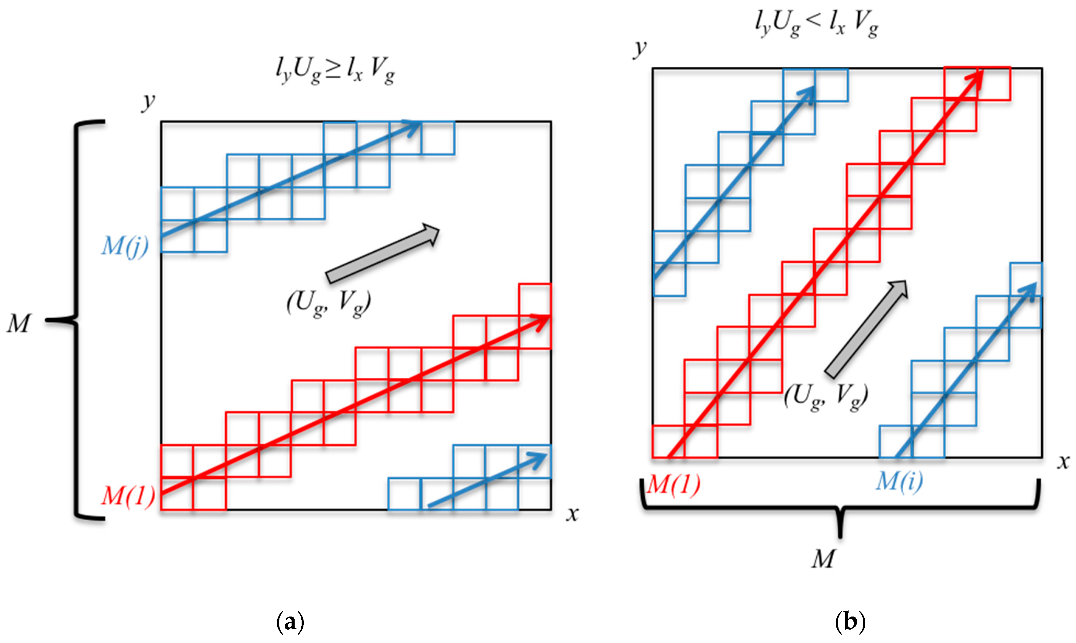
Two configurations can be found (see Figure A1a,b), depending on the relative values of lyug and lxvg. When l y U g l x V g , the integrated momentum M is computed along the y-axis for all j [ 1 , m ] , with m the number of grid points along the y-axis. Figure A1a shows the cells that will contribute to the integrated momentum M(1) (in red) and M(j) (in blue).
M r e f ( y , t ) = 0 l x ( ρ u ) ( x , y + x v r e f u r e f   m o d   l y , z r e f ) d x ,
with mod the modulo function.
The value of F(x,y,z) can be updated thanks to a generalized formulation of Table 1, with Mref defined as above. Similar derivations can be performed when l y U g < l x V g (Figure A1b).
Δ F ( x , y , t ) = ρ l x u r e f 2 + v r e f 2 ( 2 M r e f ( y , t ) M r e f ( y , t Δ t ) ) U g 2 + V g 2 Δ t l x sin θ ( z r e f ) ρ r e f ,
Figure A1. Schematic view of the two configurations for PGF4 implementation, when the wind is not aligned with a domain axis: (a) Definition for M along the y-axis; (b) definition for M along the x-axis.
Atmosphere 11 01343 g0a1

Appendix C. Validation of the Model Incorporating PGF4 against Four Experimental Datasets
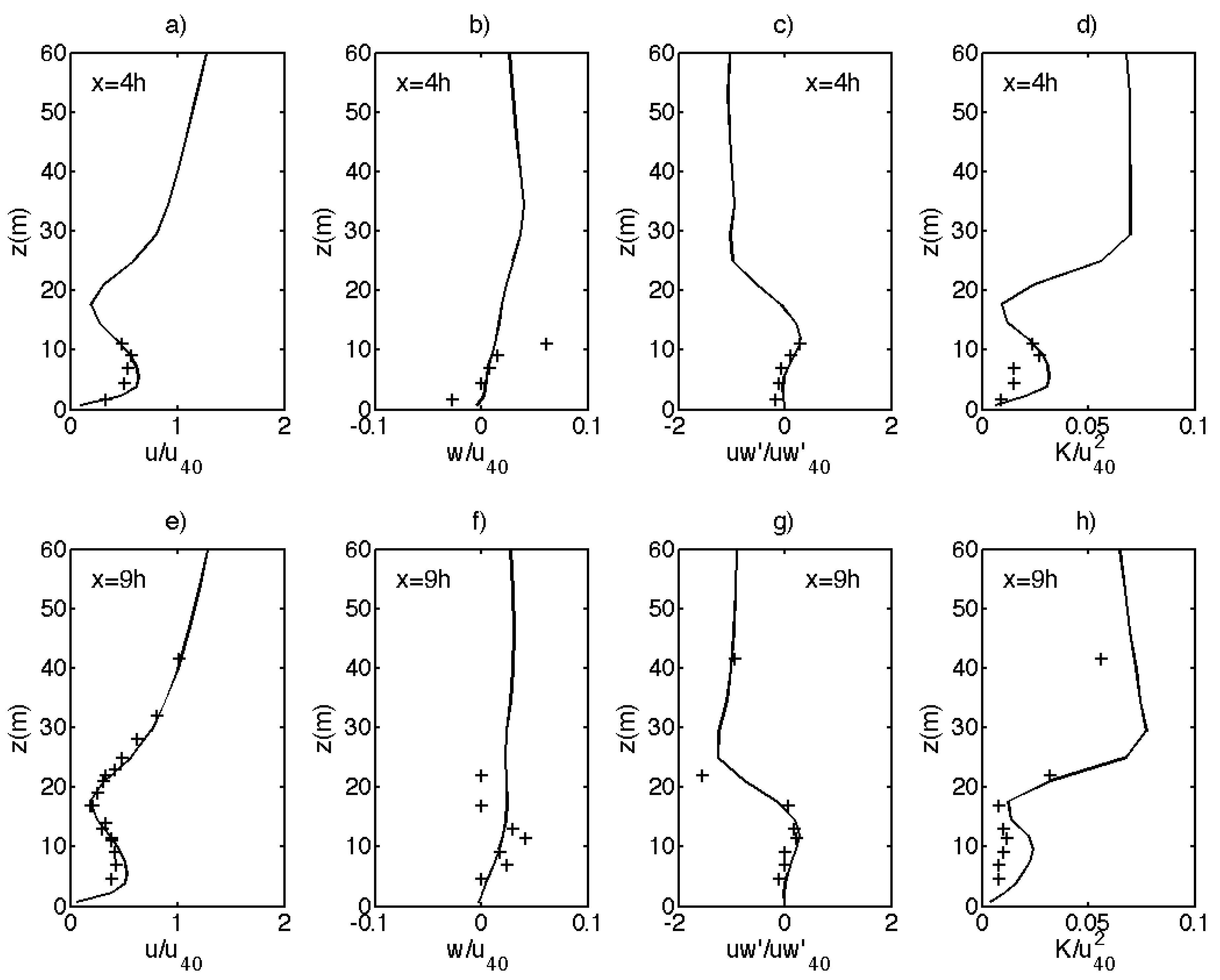
Based on the results, shown in Section 4.3, PGF4 seems to have the most desirable properties (wind velocity prescription capability, reasonable streaks). Simulations are done with PGF4 for three different canopy types (Can2, Can3, and Can4, see Table 2) to compare simulated wind statistics against experimental datasets in these four scenarios. The validation presented here does not attempt to demonstrate that the use of PGF4 improves the predictions of wind statistics compared to other pressure-gradient forcing, but that satisfactory results can be obtained with this approach too.
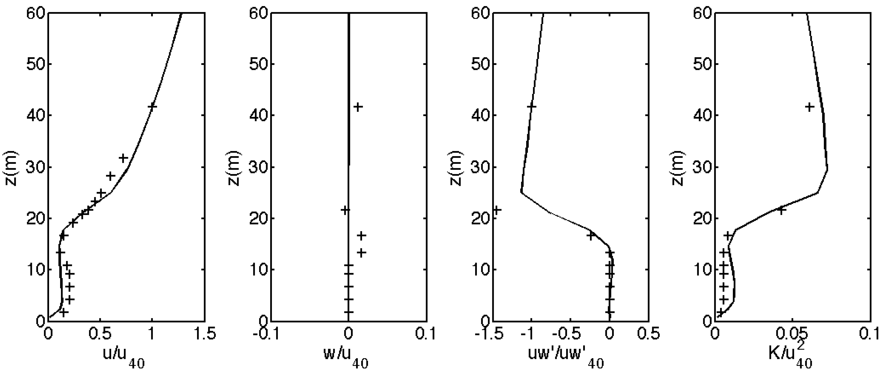
Figure A2 and Figure A3 show the profiles of u and w velocities, momentum flux, and turbulent kinetic energy, normalized by mean wind velocity at 40 m u40 for u and w velocities, by the square of the friction velocity for momentum flux, and by u402 for turbulent kinetic energy as in the study by Reference [9]. Figure A2 shows those profiles for the homogeneous forest (Can1), whereas Figure A3 shows them at two different distances from the edge (4h and 9h) in the case of the open to forest transition (Can2). The model used with PGF4 performs well with respect to reproducing experimental data. Some discrepancies can be observed: overestimation of wind velocities below the canopy in the edge case, underestimation of the momentum flux peak just above the canopy, overestimation of turbulent kinetic energy below the canopy and high above it. Similar differences are found by Reference [9], who simulated the wind flow using the Ekman balance. It is beyond the scope of the present paper to investigate the hypotheses mentioned by these authors to explain the discrepancies.
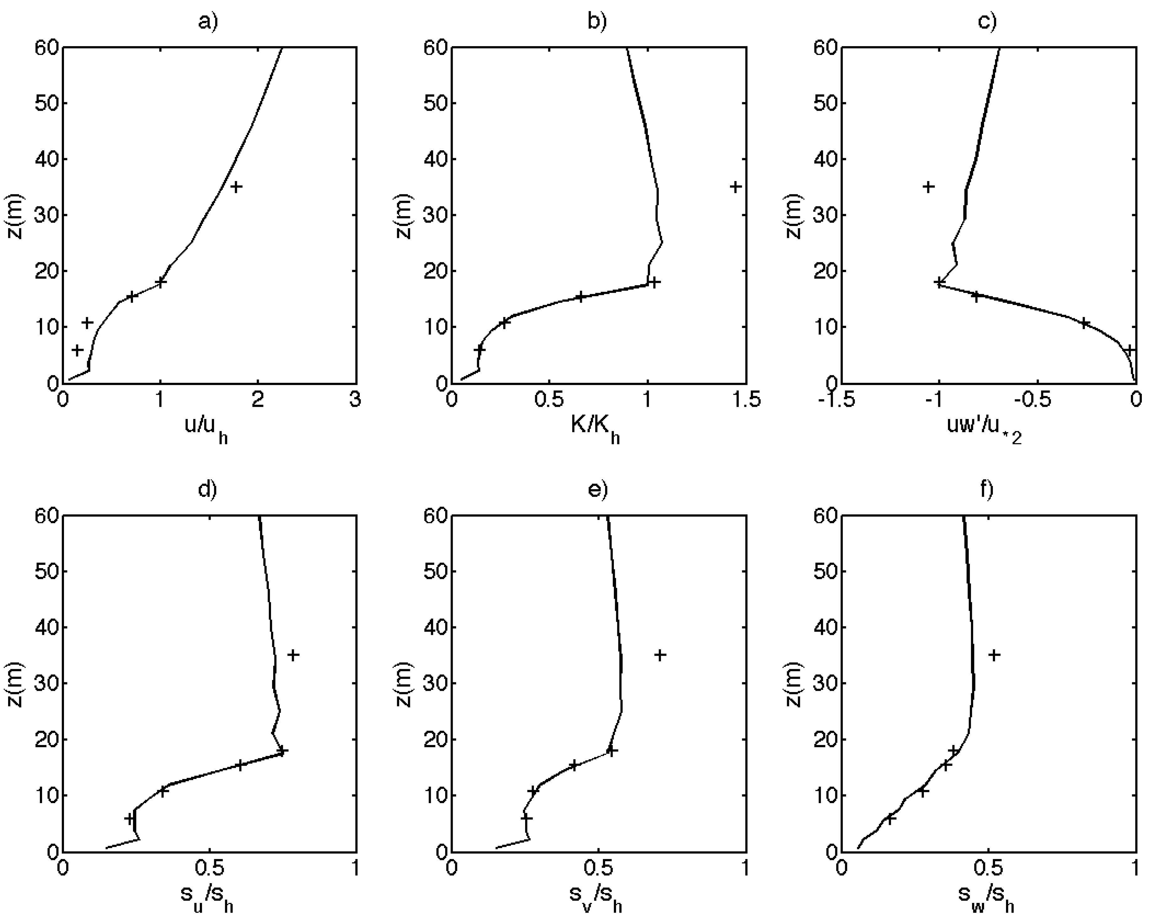
For canopy Can3, u velocity is normalized by uh (wind velocity at the canopy top, h = 18 m). Turbulent kinetic energy is normalized by its value at the canopy top (Kh). Momentum flux is normalized by the square of friction velocity. The standard deviation of u, v, and w are normalized by the standard deviation of twice the square root of turbulent kinetic energy at the canopy top (sh), as in the study by Reference [6]. Using PGF4, the model provides similar results to those by Reference [6], who did not use any pressure gradient. A similar underestimation of turbulent kinetic energy at twice the height of the canopy is observed (Figure A4).
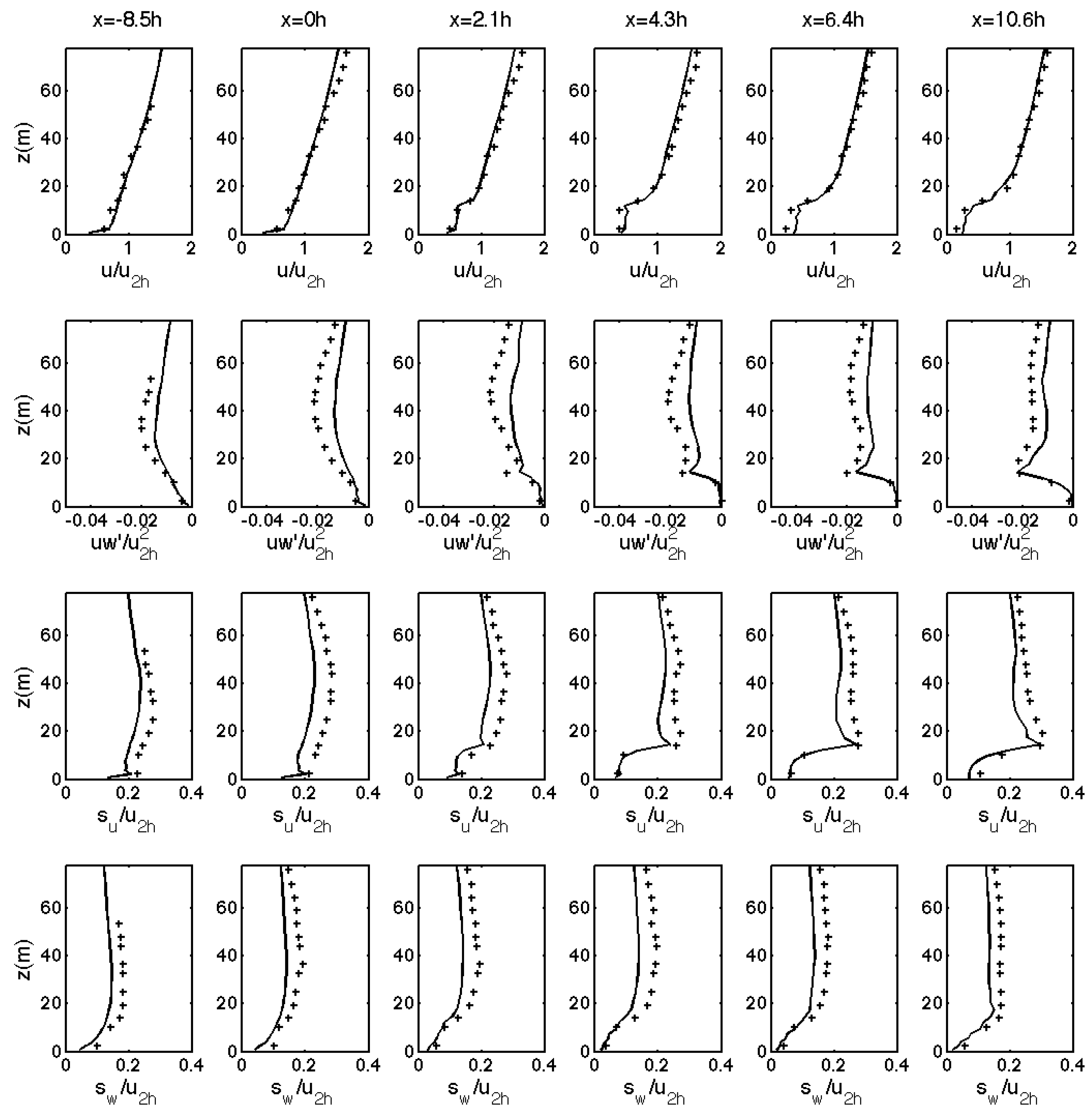
Canopy Can4 is extrapolated from a wind-tunnel experiment. The experimental dataset contains vertical wind statistic profiles at six different locations, before and after the forest edge. Mean velocity, momentum flux, the standard deviation of u and w velocities are available, and data are normalized by a single quantity u2h, which is the u velocity at twice the height of the canopy at the location of the edge (except momentum flux that is normalized by u2h2 for unit consistency). The model performance with PGF4 is found satisfactory and of equivalent quality as previous studies [6,46], with a general underestimation of turbulence quantities above the canopy (Figure A5).
Figure A2. Simulated wind statistics over canopy Can1 with PGF4 (lines), against experimental data (+’s): (a) u-velocity profile; (b) w-velocity profile; (c) momentum flux; (d) turbulent kinetic energy.
Atmosphere 11 01343 g0a2
Figure A3. Simulated wind statistics over canopy Can2 with PGF4 (lines), against experimental data (+’s) at x = 4h: (a) u-velocity profile; (b) w-velocity profile; (c) momentum flux; (d) turbulent kinetic energy; and at x = 9h: (e) u-velocity profile; (f) w-velocity profile; (g) momentum flux; (h) turbulent kinetic energy.
Atmosphere 11 01343 g0a3
Figure A4. Simulated wind statistics over canopy Can3 with PGF4 (lines), against experimental data (+’s): (a) u-velocity profile; (b) turbulent kinetic energy; (c) momentum flux; (d) standard deviation of u-velocity; (e) standard deviation of v-velocity; (f) standard deviation of w-velocity. sh is half the square root of Kh, which is turbulent kinetic energy at the canopy top.
Atmosphere 11 01343 g0a4
Figure A5. Simulated wind statistics over canopy Can4 with PGF4 (lines), against experimental data (+’s) at various location along the x-axis from −8.5 h to 10.6 h: (a) u-velocity profiles; (b) momentum fluxes; (c) standard deviation of u-velocity; (d) standard deviation of w-velocity. u2h is the mean wind velocity at z = 2 h.
Atmosphere 11 01343 g0a5

References

  1. Finnigan, J. Turbulence in Plant Canopies. Annu. Rev. Fluid Mech. 2000, 32, 519–571. [Google Scholar] [CrossRef]
  2. Pimont, F.; Dupuy, J.-L.; Linn, R.R.; Dupont, S. Impacts of tree canopy structure on wind flows and fire propagation simulated with FIRETEC. Ann. Sci. 2011, 68, 523–530. [Google Scholar] [CrossRef] [Green Version]
  3. Mueller, E.; Mell, W.; Simeoni, A. Large eddy simulation of forest canopy flow for wildland fire modeling. Can. J. Res. 2014, 44, 1534–1544. [Google Scholar] [CrossRef]
  4. Yang, B.; Raupach, M.R.; Shaw, R.H.; U, K.T.P.; Morse, A.P. Large-eddy Simulation of Turbulent Flow Across a Forest Edge. Part I: Flow Statistics. Bound. Layer Meteorol. 2006, 120, 377–412. [Google Scholar] [CrossRef]
  5. Dupont, S.; Brunet, Y. Influence of foliar density profile on canopy flow: A large-eddy simulation study. Agric. Meteorol. 2008, 148, 976–990. [Google Scholar] [CrossRef]
  6. Pimont, F.; Dupuy, J.-L.; Linn, R.R.; Dupont, S. Validation of FIRETEC wind-flows over a canopy and a fuel-break. Int. J. Wildland Fire 2009, 18, 775. [Google Scholar] [CrossRef] [Green Version]
  7. Dwyer, M.J.; Patton, E.G.; Shaw, R.H. Turbulent kinetic energy budgets from a large-eddy simulation of airflow above and within a forest canopy. Bound. Layer Meteorol. 1997, 84, 23–43. [Google Scholar] [CrossRef]
  8. Dupont, S.; Brunet, Y. Coherent structures in canopy edge flow: A large-eddy simulation study. J. Fluid Mech. 2009, 630, 93–128. [Google Scholar] [CrossRef]
  9. Dupont, S.; Bonnefond, J.-M.; Irvine, M.R.; Lamaud, E.; Brunet, Y. Long-distance edge effects in a pine forest with a deep and sparse trunk space: In situ and numerical experiments. Agric. Meteorol. 2011, 151, 328–344. [Google Scholar] [CrossRef]
  10. Nathan, R.; Sapir, N.; Trakhtenbrot, A.; Katul, G.G.; Bohrer, G.; Otte, M.; Avissar, R.; Soons, M.B.; Horn, H.S.; Wikelski, M.; et al. Long-distance biological transport processes through the air: Can nature’s complexity be unfolded in silico?: Turbulence and biological transport. Divers. Distrib. 2005, 11, 131–137. [Google Scholar] [CrossRef]
  11. Chamecki, M.; Meneveau, C.; Parlange, M.B. Large eddy simulation of pollen transport in the atmospheric boundary layer. J. Aerosol Sci. 2009, 40, 241–255. [Google Scholar] [CrossRef]
  12. Koo, E.; Linn, R.R.; Pagni, P.J.; Edminster, C.B. Modelling firebrand transport in wildfires using HIGRAD/FIRETEC. Int. J. Wildland Fire 2012, 21, 396. [Google Scholar] [CrossRef]
  13. Pimont, F.; Dupuy, J.-L.; Linn, R.R.; Parsons, R.; Martin-StPaul, N. Representativeness of wind measurements in fire experiments: Lessons learned from large-eddy simulations in a homogeneous forest. Agric. Meteorol. 2017, 232, 479–488. [Google Scholar] [CrossRef]
  14. Kanda, M.; Inagaki, A.; Letzel, M.O.; Raasch, S.; Watanabe, T. LES Study of the Energy Imbalance Problem with Eddy Covariance Fluxes. Bound. Layer Meteorol. 2004, 110, 381–404. [Google Scholar] [CrossRef]
  15. Wu, Y.-T.; Porté-Agel, F. Large-Eddy Simulation of Wind-Turbine Wakes: Evaluation of Turbine Parametrisations. Bound. Layer Meteorol. 2011, 138, 345–366. [Google Scholar] [CrossRef]
  16. Muñoz-Esparza, D.; Kosović, B.; Mirocha, J.; van Beeck, J. Bridging the Transition from Mesoscale to Microscale Turbulence in Numerical Weather Prediction Models. Bound. Layer Meteorol. 2014, 153, 409–440. [Google Scholar] [CrossRef]
  17. Muñoz-Esparza, D.; Kosović, B.; van Beeck, J.; Mirocha, J. A stochastic perturbation method to generate inflow turbulence in large-eddy simulation models: Application to neutrally stratified atmospheric boundary layers. Phys. Fluids 2015, 27, 035102. [Google Scholar] [CrossRef]
  18. Linn, R.; Anderson, K.; Winterkamp, J.; Brooks, A.; Wotton, M.; Dupuy, J.-L.; Pimont, F.; Edminster, C. Incorporating field wind data into FIRETEC simulations of the International Crown Fire Modeling Experiment (ICFME): Preliminary lessons learned. Can. J. Res. 2012, 42, 879–898. [Google Scholar] [CrossRef]
  19. Lei, L.; Stauffer, D.R.; Deng, A. A hybrid nudging-ensemble Kalman filter approach to data assimilation in WRF/DART: A Hybrid Nudging-Ensemble Kalman Filter. Q. J. R. Meteorol. Soc. 2012, 138, 2066–2078. [Google Scholar] [CrossRef]
  20. Zajaczkowski, F.J. A preliminary study of assimilating numerical weather prediction data into computational fluid dynamics models for wind prediction. J. Wind Eng. Ind. Aerodyn. 2011, 99, 320–329. [Google Scholar] [CrossRef]
  21. Allaerts, D.; Quon, E.; Draxl, C.; Churchfield, M. Development of a Time–Height Profile Assimilation Technique for Large-Eddy Simulation. Bound. Layer Meteorol. 2020, 176, 329–348. [Google Scholar] [CrossRef]
  22. Holton, J.R.; Hakim, G.J. An Introduction to Dynamic Meteorology, 5th ed.; Academic Press: Amsterdam, The Netherlands, 2013; ISBN 978-0-12-384866-6. [Google Scholar]
  23. Moeng, C.-H.; Sullivan, P.P. A Comparison of Shear- and Buoyancy-Driven Planetary Boundary Layer Flows. J. Atmos. Sci. 1994, 51, 999–1022. [Google Scholar] [CrossRef] [Green Version]
  24. Hutchins, N.; Marusic, I. Evidence of very long meandering features in the logarithmic region of turbulent boundary layers. J. Fluid Mech. 2007, 579, 1–28. [Google Scholar] [CrossRef] [Green Version]
  25. Deardorff, J.W. Stratocumulus-capped mixed layers derived from a three-dimensional model. Bound. Layer Meteorol. 1980, 18, 495–527. [Google Scholar] [CrossRef]
  26. Drobinski, P.; Foster, R.C. On the Origin of Near-Surface Streaks in the Neutrally-Stratified Planetary Boundary Layer. Bound. Layer Meteorol. 2003, 108, 247–256. [Google Scholar] [CrossRef]
  27. Foster, R.C. Structure and energetics of optimal Ekman layer perturbations. J. Fluid Mech. 1997, 333, 97–123. [Google Scholar] [CrossRef]
  28. Drobinski, P.; Brown, R.A.; Flamant, P.H.; Pelon, J. Evidence of Organized Large Eddies by Ground-Based Doppler Lidar, Sonic Anemometer and Sodar. Bound. Layer Meteorol. 1998, 88, 343–361. [Google Scholar] [CrossRef]
  29. Esau, I.N. The Coriolis effect on coherent structures in planetary boundary layers. J. Turbul. 2003, 4, N17. [Google Scholar] [CrossRef]
  30. Shaw, R.H.; Schumann, U. Large-eddy simulation of turbulent flow above and within a forest. Bound. Layer Meteorol. 1992, 61, 47–64. [Google Scholar] [CrossRef] [Green Version]
  31. Patton, E.G. Large-Eddy Simulation of Turbulent Flow Above and within a Plant Canopy. Ph.D. Thesis, University of California Davis, Davis, CA, USA, 1997. [Google Scholar]
  32. Patton, E.G.; Shaw, R.H.; Judd, M.J.; Raupach, M.R. Large-Eddy Simulation of Windbreak Flow. Bound. Layer Meteorol. 1998, 87, 275–307. [Google Scholar] [CrossRef]
  33. Su, H.-B.; Shaw, R.H.; Paw, K.T.; Moeng, C.-H.; Sullivan, P.P. Turbulent Statistics of Neutrally Stratified Flow Within and Above a Sparse Forest from Large-Eddy Simulation and Field Observations. Bound. Layer Meteorol. 1998, 88, 363–397. [Google Scholar] [CrossRef]
  34. Huang, J.; Cassiani, M.; Albertson, J.D. Analysis of Coherent Structures within the Atmospheric Boundary Layer. Bound. Layer Meteorol. 2009, 131, 147–171. [Google Scholar] [CrossRef]
  35. Lu, H.; Porté-Agel, F. A modulated gradient model for large-eddy simulation: Application to a neutral atmospheric boundary layer. Phys. Fluids 2010, 22, 015109. [Google Scholar] [CrossRef] [Green Version]
  36. Munters, W.; Meneveau, C.; Meyers, J. Shifted periodic boundary conditions for simulations of wall-bounded turbulent flows. Phys. Fluids 2016, 28, 025112. [Google Scholar] [CrossRef] [Green Version]
  37. Fishpool, G.M.; Lardeau, S.; Leschziner, M.A. Persistent Non-Homogeneous Features in Periodic Channel-Flow Simulations. Flow Turbul. Combust. 2009, 83, 323–342. [Google Scholar] [CrossRef]
  38. Reisner, J.; Wynne, S.; Margolin, L.; Linn, R. Coupled Atmospheric–Fire Modeling Employing the Method of Averages. Mon. Weather Rev. 2000, 128, 3683–3691. [Google Scholar] [CrossRef]
  39. Linn, R.R. Numerical simulations of grass fires using a coupled atmosphere–fire model: Basic fire behavior and dependence on wind speed. J. Geophys. Res. 2005, 110. [Google Scholar] [CrossRef]
  40. Raupach, M.R.; Bradley, E.F.; Ghadiri, H. A Wind Tunnel Investigation into the Aerodynamic Effect of Forest Clearings on the Nesting of Abbott’s Booby on Christmas Island: Progress Report on a Study Commissioned by the Australian National Parks and Wildlife Service; CSIRO Division of Environmental Mechanics: Canberra, Australia, 1987. [Google Scholar] [CrossRef]
  41. Muñoz-Esparza, D.; Kosović, B.; García-Sánchez, C.; van Beeck, J. Nesting Turbulence in an Offshore Convective Boundary Layer Using Large-Eddy Simulations. Bound. Layer Meteorol. 2014, 151, 453–478. [Google Scholar] [CrossRef]
  42. Watanabe, T. Large-Eddy Simulation of Coherent Turbulence Structures Associated with Scalar Ramps over Plant Canopies. Bound. Layer Meteorol. 2004, 112, 307–341. [Google Scholar] [CrossRef]
  43. Smith, F.B.; Carson, D.J.; Oliver, H.R. Mean wind-direction shear through a forest canopy. Bound. Layer Meteorol. 1972, 3, 178–190. [Google Scholar] [CrossRef]
  44. Wilson, J.D.; Flesch, T.K. Wind and remnant tree sway in forest cutblocks. III. A windflow model to diagnose spatial variation. Agric. Meteorol. 1999, 93, 259–282. [Google Scholar] [CrossRef]
  45. Fang, J.; Porté-Agel, F. Large-Eddy Simulation of Very-Large-Scale Motions in the Neutrally Stratified Atmospheric Boundary Layer. Bound. Layer Meteorol. 2015, 155, 397–416. [Google Scholar] [CrossRef] [Green Version]
  46. Dupont, S.; Brunet, Y. Edge Flow and Canopy Structure: A Large-Eddy Simulation Study. Bound. Layer Meteorol. 2007, 126, 51–71. [Google Scholar] [CrossRef]
  47. Patton, E.G.; Sullivan, P.P.; Davis, K.J. The influence of a forest canopy on top-down and bottom-up diffusion in the planetary boundary layer. Q. J. R. Meteorol. Soc. 2003, 129, 1415–1434. [Google Scholar] [CrossRef]
  48. Dupont, S.; Brunet, Y.; Finnigan, J.J. Large-eddy simulation of turbulent flow over a forested hill: Validation and coherent structure identification. Q. J. R. Meteorol. Soc. 2008, 134, 1911–1929. [Google Scholar] [CrossRef]
  49. Pimont, F.; Dupuy, J.-L.; Linn, R.R. Fire effects on the physical environment in the WUI using FIRETEC. In Advances in Forest Fire Research; Imprensa da Universidade de Coimbra: Coimbra, Portugal, 2014; pp. 749–758. ISBN 978-989-26-0884-6. [Google Scholar]
  50. Raupach, M.R. Simplified expressions for vegetation roughness length and zero-plane displacement as functions of canopy height and area index. Bound. Layer Meteorol. 1994, 71, 211–216. [Google Scholar] [CrossRef]
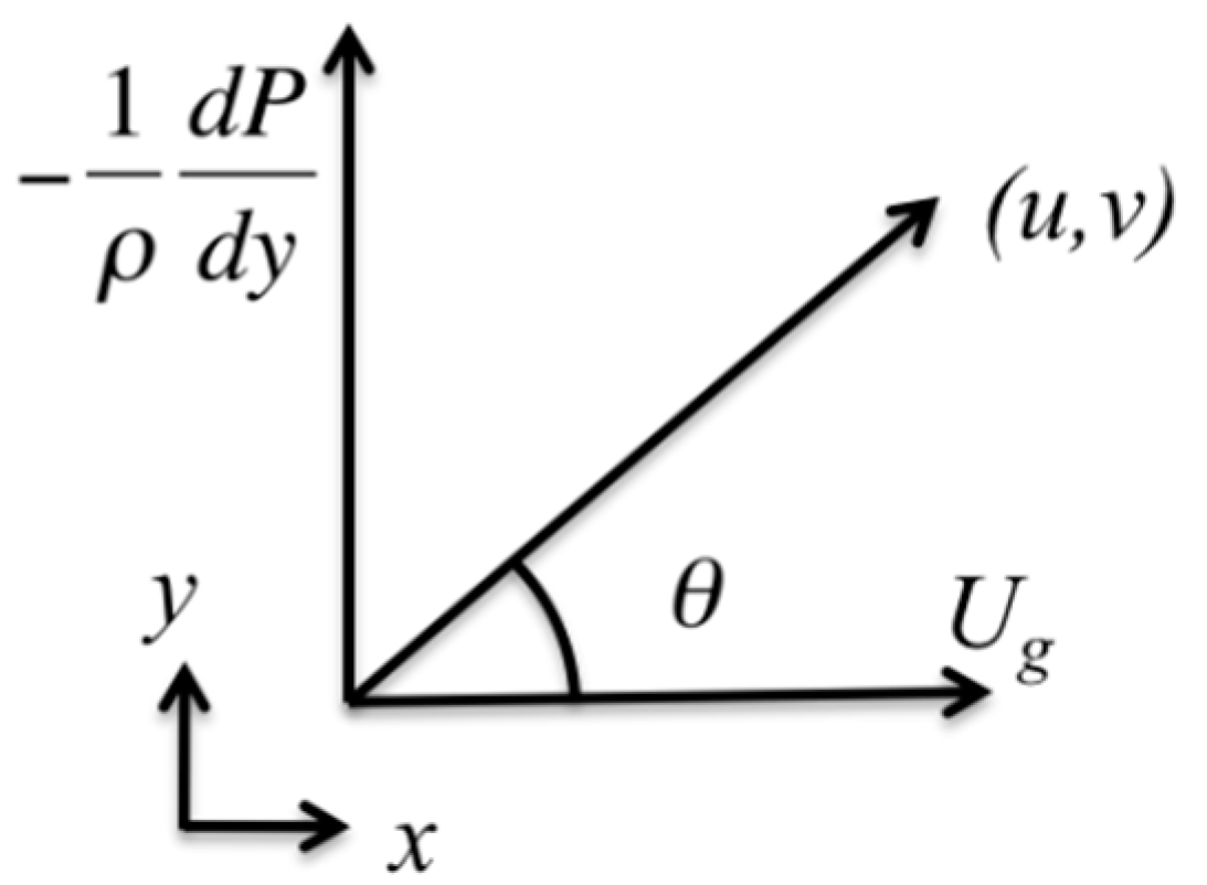
Figure 1. Projection of the geostrophic wind on the wind direction.
Atmosphere 11 01343 g001
Figure 2. sin θ ( z ) profile (Equation (9)) using Ekman’s assumptions and γ = π 600 .
Atmosphere 11 01343 g002
Figure 3. Vertical profiles of normalized turbulent statistics for the sensitivity-analysis simulations: (a) Mean streamwise velocity; (b) modeled and experimental wind velocities below 60 m; (c) turbulent kinetic energy; (d) momentum flux. U 40 and U w 40 are the horizontal wind velocity and momentum flux at z = 40 m.
Atmosphere 11 01343 g003
Figure 4. Spectral analysis of the u-velocity component for the sensitivity-analysis simulations, at (a) z = 15 m, (b) z = 50 m, (c) z = 80 m and (d) z = 200 m.
Atmosphere 11 01343 g004
Figure 5. Temporal evolution of the instantaneous profiles of the spatially-averaged horizontal streamwise velocities for the boundary-layer simulations (1568 m × 1568 m × 800 m): (a) EKBS; (b) CPGF; (c) PGF1; (d) PGF2; (e) PGF3; (f) PGF4. Instantaneous profiles are printed every 200 s and averaged along the x- and y-axes. Profile colors are associated with a range of simulated time: 0–4000 s in blue, 4000–6000 s in green, 6000–8000 s in red, 8000–10,000 s in cyan, 10,000–12,000 s in purple. Note that a different range is used for CPGF, due to a longer time required for convergence.
Atmosphere 11 01343 g005
Figure 6. Vertical profiles of normalized turbulent statistics for the boundary-layer simulations (1568 m × 1568 m × 800 m): (a) Mean streamwise velocity; (b) wind velocity up to 300 m; (c) turbulent kinetic energy; (d) momentum flux. U 40 and U w 40 are the horizontal wind velocity and momentum flux at z = 40 m.
Atmosphere 11 01343 g006
Figure 7. Instantaneous horizontal wind velocities on a horizontal plane at z = 56 m and t = 10,800 s for the boundary-layer simulations (1568 m × 1568 m × 800 m): (a) EKBS; (b) CPGF; (c) PGF1; (d) PGF2; (e) PGF3; (f) PGF4. For each simulation, wind velocities are normalized by the mean wind velocity at z = 56 m.
Atmosphere 11 01343 g007
Figure 8. One-hour-averaged horizontal wind velocities on a horizontal plane at z = 56 m for the boundary-layer simulations (1568 m × 1568 m × 800 m): (a) EKBS; (b) CPGF; (c) PGF1; (d) PGF2; (e) PGF3; (f) PGF4. For each simulation, wind velocities are normalized by the mean wind velocity at z = 56 m.
Atmosphere 11 01343 g008
Figure 9. Spectral analysis of the u-velocity component for the boundary-layer simulations (1568 m × 1568 m × 800 m), at (a) z = 15 m, (b) z = 80 m, (c) z = 250 m and (d) z = 350 m. The black-point line represents the −2/3 power line.
Atmosphere 11 01343 g009
Figure 10. Vertical profiles of normalized turbulent statistics for the canopy-flow simulations (512 m × 512 m × 615 m): (a) Mean streamwise velocity up to 400 m; (b) mean streamwise velocity up to 100 m; (c) turbulent kinetic energy up to 100 m; (d) momentum flux up to 100 m. U40 and Uw40 are the horizontal wind velocity and momentum flux at z = 40 m.
Atmosphere 11 01343 g010
Figure 11. One-hour-averaged horizontal wind velocities on a horizontal plane at z = 53 m for the canopy-flow simulations (512 m × 512 m × 615 m): (a) EKBD, (b) CPGF, (c) PGF1, (d) PGF2, (e) PGF4, (f) subset of EKBD1536x615dx4 simulations, for reference. For each simulation, wind velocities are normalized by the mean wind velocity at z = 53 m.
Atmosphere 11 01343 g011
Figure 12. Spectral analysis of the u-velocity component for the wildfire-precursor simulations (512 m × 512 m × 615 m) and EKBD1536x615dx4 for reference, at (a) z = 15 m, (b) z = 50 m, (c) z = 80 m and (d) z = 200 m. The black-point line represents the −2/3 power line.
Atmosphere 11 01343 g012
Table 1. Description of the different forcing corresponding to a geostrophic wind U g i (with i the unit vector of the x-axis). zref is the reference height where velocity uref is targeted, ρ r e f is air density at zref, sin θ is defined according to Equation (9) and lx, ly, lz are the extents of the domain along the x, y and z-axes. Except for the Ekman balance (EKB), the forcing (CPGF or PGFs) is applied to the u-momentum equation (streamwise).
ModeForcingForcing UpdateIntegrated Momentum
EKB f v and f ( U g u ) in x and y directionNoNo
CPGF F ( t ) If M ( t ) > M e q ,   Δ F ( t ) < 0
Else Δ F ( t ) > 0
M ( t ) = x , y , z l x l y l z ρ u d x d y d z
PGF1 F ( t ) U g sin θ ( z ) Δ F ( t ) = M e q ( 2 M ( t ) M ( t Δ t ) ) U g Δ t l x l y 0 l z ρ sin θ d z M ( t ) = x , y , z l x l y l z ρ u d x d y d z
PGF2 F r e f ( t ) U g sin θ ( z ) Δ F r e f ( t ) = ρ l x l y u r e f ( 2 M r e f ( t ) M r e f ( t Δ t ) ) U g Δ t l x l y sin θ ( z r e f ) ρ r e f M r e f ( t ) = x , y l x l y ( ρ u ) ( x , y , z r e f ) d x d y
PGF3 F ( y , t ) U g sin θ ( z ) Δ F ( y , t ) = M e q ( 2 M ( y , t ) M ( y , t Δ t ) ) l y U g Δ t l x l y 0 l z sin ρ θ d z M ( y , t ) = x , z l x l z ( ρ u ) ( x , y , z r e f ) d x d z
PGF4 F r e f ( y , t ) U g sin θ ( z ) Δ F r e f ( y , t ) = ρ l x u r e f ( 2 M r e f ( y , t ) M r e f ( y , t Δ t ) ) U g Δ t l x sin θ ( z r e f ) ρ r e f M r e f ( y , t ) = x = 0 l x ( ρ u ) ( x , y , z r e f ) d x
Table 2. Description of the four canopy configurations used in the present study.
ScenarioCanopy TypeReferenceCanopy Height and LAI; Structure
Can1Homogeneous, maritime pine[9]h = 22 m and LAI = 2
Can2Forest edge, maritime pine[9]h = 22 m and LAI = 2; 200 m open
Can3Deciduous forest[6]h = 18 m and LAI = 2
Can4Extrapolated from wind tunnel, forest edge[6,40]h = 13.3 m and LAI = 2; 394 m open
Table 3. Description of grid configurations and timesteps used in the present study. d z ¯ is the mean cell height (m), a z the vertical stretching factor (roughly equals to d z ( 1 ) d z ¯ ) and n the cell number in the vertical. The vertical stretching is given by d z ( k ) = d z ¯ ( a z + 3 ( 1 a z ) ( k n z ) 2 ) , with k the vertical index. dt is the small timestep of the Method of Averages (Reisner 2000). The two reference simulations are in the bold.
Grid NamesDomain Extents (m)dx, dy (m) d z ¯   ( m ) aznzdt (s)
3136x800dx83136 × 3136 × 8008100.4800.004
1568x800dx8 11568 × 1568 × 8008100.4800.004
1568x615dx41568 × 1568 × 6154150.1410.002
768x615dx2768 × 512 × 6152150.1410.002
512x615dx2 2512 × 512 × 6152150.1410.002
256x615dx2256 × 256 × 6152150.1410.002
512x199dx2512 × 512 × 19927.350.2270.002
512x106dx2512 × 512 × 106250.3210.002
256x106dx2256 × 256 × 106250.3210.002
1Reference boundary-layer flow simulation;2Reference wildfire-precursor simulation.
Table 4. Description of the main characteristics of the simulations.
SimulationPressure-Gradient ForcingUpper BoundaryCanopy
EKBS_3136x800dx8Ekman balanceGeostrophic wind, capping inversionCan1
EKBS_1568x800dx8Ekman balanceGeostrophic wind, capping inversionCan1
CPGF_1568x800dx8Constant pressure gradientFree slip, capping inversionCan1
PGF1_1568x800dx8PGF1Geostrophic wind, capping inversionCan1
PGF2_1568x800dx8PGF2Geostrophic wind, capping inversionCan1
PGF3_1568x800dx8PGF3Geostrophic wind, capping inversionCan1
PGF4_1568x800dx8PGF4Geostrophic wind, capping inversionCan1
EKBD_1568x615dx4Ekman balanceRayleigh damperCan1
EKBD_512x615dx2Ekman balanceRayleigh damperCan1
CPGF_512x615dx2Constant pressure gradientFree slipCan1
PGF1_512x615dx2PGF1Rayleigh damperCan1
PGF2_512x615dx2PGF2Rayleigh damperCan1
PGF3_512x615dx2PGF3Rayleigh damperCan1
PGF4_512x615dx2PGF4Rayleigh damperCan1
PGF4_512x615dx2_Can2PGF4Rayleigh damperCan2
PGF4_512x615dx2_Can3PGF4Rayleigh damperCan3
PGF4_768x615dx2_Can4PGF4Rayleigh damperCan4
EKBD_256x615dx2Ekman balanceRayleigh damperCan1
CPGF_512x199dx2Constant pressure gradientFree slipCan1
CPGF_512x106dx2Constant pressure gradientFree slipCan1
CPGF_256x106dx2Constant pressure gradientFree slipCan1
Table 5. Mean wind velocity at zref = 40 m. The target wind speed is 3 m s−1.
Simulation U 40 (m s−1)
EKBS_1568x800dx82.24
CPGF_1568x800dx81.67
PGF1_1568x800dx82.42
PGF2_1568x800dx83.02
PGF3_1568x800dx82.25
PGF4_1568x800dx83.03
EKBS_512x615dx22.04
CPGF_512x615dx22.34
PGF1_512x615dx22.29
PGF2_512x615dx23.04
PGF3_512x615dx22.17
PGF4_512x615dx22.98
Publisher’s Note: MDPI stays neutral with regard to jurisdictional claims in published maps and institutional affiliations.