Article

Performance Evaluation of an Operational Rapid Response Fire Spread Forecasting System in the Southeast Mediterranean (Greece)

by
Theodore M. Giannaros
*,
Konstantinos Lagouvardos
and
Vassiliki Kotroni
National Observatory of Athens, Institute for Environmental Research and Sustainable Development, Lofos Koufou, 15236 Penteli, Greece
*
Author to whom correspondence should be addressed.
Atmosphere 2020, 11(11), 1264; https://doi.org/10.3390/atmos11111264
Submission received: 12 October 2020 / Revised: 17 November 2020 / Accepted: 18 November 2020 / Published: 23 November 2020
(This article belongs to the Special Issue Coupled Fire-Atmosphere Simulation)

Abstract

:
The current work presents the operational implementation and evaluation of a rapid response fire spread forecasting system, named IRIS, that was developed to provide support to the tactical wildfire suppression activities of the Hellenic Fire Corps. The system was operationally employed during the 2019 fire season in Greece, providing on-demand wildfire spread predictions for 17 incidents. Satellite remote sensing data were employed for quantitatively assessing IRIS’s predictions for eight selected events. Our results suggest an overall satisfactory model performance. More importantly, this study demonstrates that, as coupled fire-atmosphere modeling becomes an increasingly popular approach, the respective models have great potential to support operational agencies and wildfire managers during the incident phase.

1. Introduction

Wildfires are an integral component of many terrestrial biomes [1], including Mediterranean ecosystems [2]. It is estimated that every year, an average ~45,000 wildfires occur in the Mediterranean [3], generating approximately 85% of the total burnt area (BA) of Europe [4]. A proportion of these wildfires are associated with an increased risk of direct damages to humans and properties [5], and adverse primary and secondary environmental impacts (e.g., soil erosion) [6]. Such catastrophic wildfires have repeatedly affected the Mediterranean countries in recent decades [7]. For instance, the wildfires that broke out in Portugal in 2003, caused the death of 21 people and induced damages estimated at over 1 billion Euro [8], while most recently, in 2018, 103 people lost their lives in the deadliest wildfire in the modern history of Greece [9]. The growing concern about wildfires and their adverse consequences is further supported by the increasing trends in both their frequency of occurrence and spatial extent, as a result of climate change [10] and other anthropogenic factors, such as the expansion of the wildland-urban interface [11].
To contain the socio-economic impacts of wildfires, policymakers, land managers, and operational firefighting agencies must rely on information related to wildfire spread and behavior [12]. Such information is critically important for wildfire management, particularly with respect to evaluating the most effective tactical wildfire suppression options during the incident support phase [13]. Numerical models, able to simulate the perimeter growth and behavior of wildfires, are thus considered to be a highly valuable tool.
The numerical modeling of wildfire spread and behavior dates back to the early 1970s when the first models were developed to understand observed incidents, predict wildfire spread, and evaluate the influence of varying environmental conditions on wildfire behavior [14]. Today, the wide array of available models ranges from advanced 3D computational fluid dynamics and combustion models such as FIRETEC [15] and WFDS (Wildland-Urban Interface Fire Dynamics Simulator) [16] to empirical models such as FARSITE [17] and BehavePlus [18]. Each model is characterized by certain advantages and disadvantages, all related to computational demands, data requirements, accuracy, robustness, and transferability [19].
From an operational point of view, the fundamental requirement is to achieve a balance between the physics and the overall complexity of a wildfire simulator, which ultimately affects its accuracy and computational cost. Purely physical models [15,16] are considered to be among the most accurate, operating at very fine spatial resolutions and resolving the combustion processes. However, these models are also the most inappropriate for operational applications, as they demand a large computational effort that limits their implementation to small simulation domains or/and coarse representations of the landscape characteristics [20]. Even if computational restrictions did not exist, the full exploitation of the capabilities of such models would require the availability of extremely high-resolution input data (e.g., fuel type and condition, topography), which are rarely available for real-time applications. On the other extreme, empirical and semi-empirical models [17,18] are the most computationally efficient and have been shown to provide accurate wildfire spread predictions, even outside of the limits of their training datasets [21]. In between, there exists the approach of coupling a numerical weather prediction (NWP) model with a 2D wildfire spread model. Coupled fire-atmosphere models are considered as an intermediate trade-off, providing the necessary balance between the realism of the represented physical processes and the computational demands for performing real-time predictions [22,23,24].
While adapted to a real-time response, coupled fire-atmosphere models have been proven to be able to reproduce wildfire spread [22,23,24,25,26,27,28,29,30] and smoke dispersion [31,32,33], and even anticipate several dynamic, transient phenomena, such as convective plumes, fire-induced winds, and horizontal roll vortices [34,35,36,37]. Nevertheless, such models are still not widely used in wildfire incident management. Instead, the common practice is to use an empirical model driven by external meteorological forcing [13,38,39,40]. Although this is an efficient approach, it presents several limitations. For instance, the wind field driving wildfire spread is provided by an external meteorological model that typically operates at a spatial resolution that is insufficient for resolving local effects of topography. Finer resolution wind fields could be obtained by employing a diagnostic model based on mass conservation [41,42], but this approach would not increase the temporal resolution of the primary meteorological forcing (typically 1 h). Most importantly, the use of the external meteorological forcing does not allow for considering the significant two-way interactions between the fire and the atmosphere (i.e., “the fire creates its own weather”).
In this work, we present the operational implementation of a rapid response fire spread forecasting system. Named IRIS, after a messenger goddess in Greek mythology, the forecasting system was developed to provide operational support to the Hellenic Fire Corps (HFC) and is currently, to the best of our knowledge, the first of its kind in the European Union (EU). The system was developed under the framework of the DISARM (Drought and fIre obServatory and eArly waRning systeM) project which used state-of-the-art observational and modeling techniques for building a common prevention and mitigation framework for the vulnerable region of the southeast Mediterranean [43]. IRIS is based on the coupled fire-atmosphere WRF-Fire model [44], properly adapted to account for the pyric environment of Greece [24]. IRIS was operationally deployed in Greece during the 2019 fire season, providing real-time, on-demand wildfire spread predictions for 17 incidents in total. Satellite-based remote sensing data were employed for assessing the accuracy of the system’s predictions and evaluating its overall performance. Our overarching goal is to demonstrate that IRIS, a coupled fire-atmosphere modeling system, has great potential to effectively support tactical wildfire suppression planning through the provision of added-value forecast guidance. Compared to previous studies that employed coupled fire-atmosphere models, our work differs in the sense that it considers several events for providing a quantitative and qualitative performance evaluation of the model. Therefore, we believe that this study is one of the first, if not the first, to introduce a detailed accuracy assessment of an operational fire spread forecasting system that is based on coupled fire-atmosphere modeling.

2. Methodology and Data

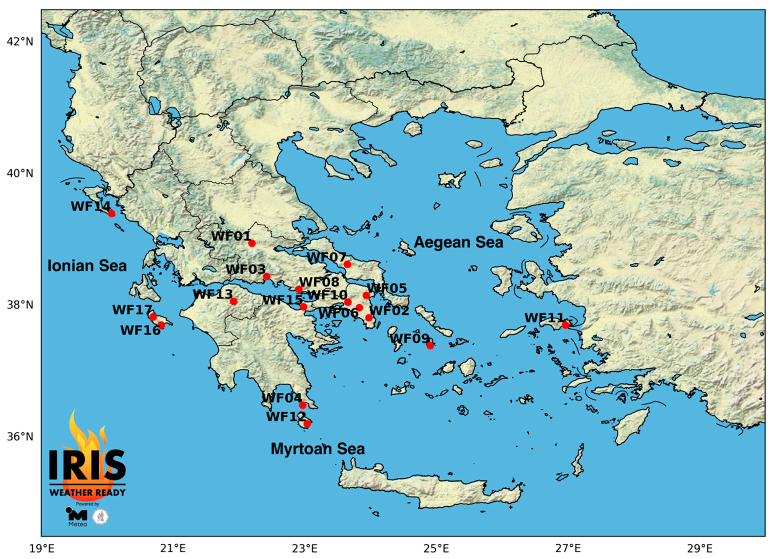
2.1. Study Area, Selected Wildfires and Data

IRIS was designed and developed to operationally support wildfire suppression activities of the HFC in Greece. The country is located between 34° and 42° northern latitude, and 19° and 28° eastern longitude in southeast Europe, covering an area of approximately 132,000 km2. Although Greece has one of the longest coastlines in the world, due to the numerous islands and highly indented coastline, mountains and hills represent about 80% of its total surface. The dominant vegetation types affected by wildfires include phryganic ecosystems, Pinus halepensis and Pinus brutia forests, Quercus coccifera shrublands, and Mediterranean grasslands, which collectively cover up to ~39% of the country’s surface [45].
During the 2019 fire season (1 May–31 October), IRIS was operationally deployed by the HFC on 17 occasions in total. The locations of the wildfires for which the forecasting system was activated are shown in Figure 1. The vast majority of the incidents took place in southern Greece, as expected given the wildfire climatology of Greece [46]. Out of the 17 wildfires, 11 occurred in mainland Greece and 6 burned across islands of the Ionian, Myrtoan, and Aegean Sea. August was the busiest month for IRIS (11 incidents), followed by July (3 incidents) and September (3 incidents).
Table 1 summarizes key information about the eight most significant wildfires of the 2019 fire season, for which IRIS was activated and provided spread predictions, and for which satellite remote sensing data were available for carrying out the predictions’ evaluation. According to the official records of the HFC [47], the cumulative BA of the selected events (5767 ha) accounted for approximately 56% of the 2019 fire season total BA in Greece (~10,338 ha). The largest incident was inarguably the Kontodespoti wildfire (WF07), which burned more than 2500 ha in about 39 h, followed by the Lithakia (WF16), Prodromos (WF08), and Elafonissos (WF04) wildfires, which burned more than 500 ha. On the other hand, the two smallest events were those that took place in Mesokampos (WF11) and Kastri (WF01), burning less than 100 ha. The remaining two events, in Hymettus (WF06) and Loutraki (WF15), were important mostly due to their proximity to populated residential areas. All incidents, except WF04 and WF07, lasted for less than 24 h. The reported events’ durations do not include the time spent for mop-up operations, thus considering only the time of active wildfire spread. This information was either provided by HFC officers or retrieved from news reports.
For the evaluation of IRIS’s predictions, wildfire perimeter data were retrieved from the European Forest Fire Information System (EFFIS) [48]. These data have a spatial resolution of about 250 × 250 m2 and are based on measurements taken from the MODIS (Moderate Resolution Imaging Spectroradiometer) instrument onboard the Terra and Aqua satellites. In addition, wind speed and direction observations were used for evaluating IRIS’s wind forecasts. These data were retrieved from the network of automatic weather stations (AWSs) that the National Observatory of Athens (NOA) has operated in Greece since 2007 [49]. Depending on the ignition location of each wildfire, we obtained wind speed and direction measurements from the nearest AWS with data availability (Table 2). Unfortunately, the selected AWS may not always be representative of the meteorological conditions prevailing in the vicinity of the wildfires. However, their observations are considered to be useful for evaluating the overall model performance with respect to wind forecasting.

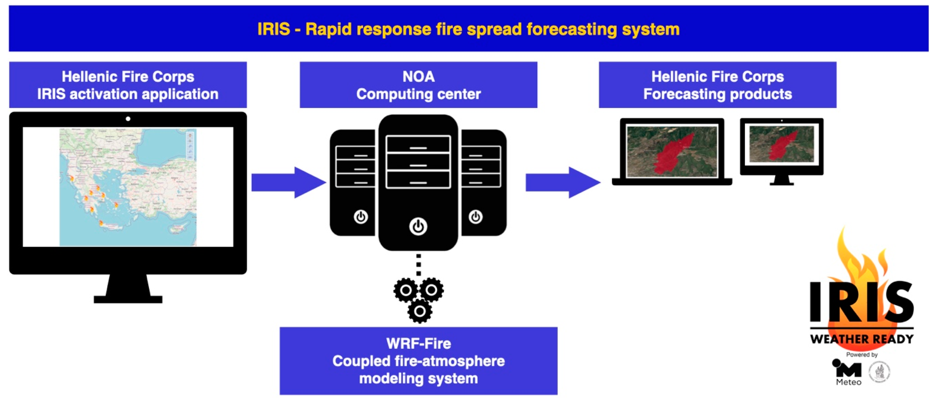
2.2. IRIS—Rapid Response Fire Spread Forecasting System

Figure 2 presents the flow chart of the IRIS rapid response fire spread forecasting system, as it was operationally implemented in Greece during the 2019 fire season. The on-demand deployment of the system is exclusively controlled by officers of the HFC through a password-protected web application. This application allows HFC officers to navigate through the map of Greece and request the activation of IRIS by simply clicking on the map, providing the coordinates and time of ignition. As soon as a wildfire is registered on the web application, a daemon running on NOA’s computational infrastructure triggers the execution of WRF-Fire, launching a shell script that takes the ignition coordinates and time as arguments. The latter is employed for automatically setting up the simulation domains and initializing the coupled fire-atmosphere modeling system (Section 2.2.1). To ensure the timely delivery of the wildfire spread forecasts, WRF-Fire is currently implemented on 5 Intel Xeon Gold 6148 computing nodes, interconnected with FDR InfiniBand. Each node has two 20-core CPUs, resulting in total computing power of 200 cores. Forecasts are communicated to the HFC through email, in Google Earth KMZ and ESRI Shapefile formats. The 24 h wildfire spread prediction is provided in about 1 h following the activation of IRIS, while the first 6 h of the forecast are provided in approximately 15–20 min. It is worth noticing that the entire execution chain of IRIS is fully automated, requiring no human intervention at any point.

2.2.1. The WRF-Fire Coupled Fire-Atmosphere Modeling System

The 2019 version of IRIS, presented herein, is an update of the previous version that Giannaros et al. [24] presented in detail. Compared to its predecessor, the new system is based on the WRF-Fire coupled fire-atmosphere modeling system version 4.0.2 [44], a quasi-physical wildfire simulator that resolves the physics of the fire and fire-atmosphere interactions but does not consider the chemistry of combustion. Wildfire spread is simulated with the semi-empirical algorithm of Rothermel [50], applied within the computational framework of a high-order level-set method that uses a fifth-order WENO (Weighted Essentially Non-Oscillatory) method for the discretization of spatial derivatives, and a third-order Runge-Kutta temporal integration [44]. For the computation of the rate of spread (ROS), the properties of the burning fuels, and meteorological and terrain (slope) data are used. The coupling between the fire and the atmosphere takes place through the sensible and latent heat fluxes released by the wildfire. Simply put, the atmosphere of WRF-Fire “feels” the fire and responds by adjusting air temperature and humidity, pressure, density, and wind. For a more detailed description of WRF-Fire, the interested reader is advised to refer to [44,51].
Within IRIS, WRF-Fire is configured to run on 3 two-way nested modeling domains with horizontal grid spacings of 25 km (DO1; mesh size of 120 × 120), 5 km (DO2; mesh size of 121 × 121), and 1 km (DO3; mesh size of 151 × 151). All domains are telescopically nested with the location of the wildfire ignition found at their center. In the vertical, 41 unevenly spaced, hybrid, terrain-following sigma-pressure levels are defined, with the model top set to 50 hPa. The default terrestrial datasets distributed with the WRF model [52] are used for the representation of land use, topography, and soil type. Shortwave and longwave radiation are parameterized with the RRTMG (Rapid Radiative Transfer Model) scheme [53], and microphysics are represented with the Thompson parameterization [54]. The planetary boundary-layer is parameterized with the Yonsei University (YSU) scheme [55], coupled with the revised MM5 scheme [56] for parameterizing surface-layer processes. Land-surface processes are represented with the Unified NOAH land-surface model [57], and the Grell-Freitas ensemble scheme [58] is used for parameterizing convection in DO1 and DO2 (convection is resolved explicitly in DO3).
The simulation of the wildfire spread is carried out on an ultra-high-resolution modeling domain, embedded as a sub-grid in DO3. A grid refinement ratio of 10:1 is adopted, resulting in a fire domain with a horizontal grid spacing of 100 m (mesh size of 1501 × 1501). This particular spatial resolution was chosen based on the resolution of the terrestrial datasets that are available for its initialization. Specifically, these include terrain elevation data, which is used for deriving slope, and fuels’ data. For topography, the 90 m resolution SRTM (Shuttle Radar Topography Mission) data [59] are used. For the representation of fuels, the 100 m resolution prototype fuel map of Greece, constructed by Giannaros et al. [24], was employed. More details on the latter are available in [24].
For the initialization of WRF-Fire, the 0.25° × 0.25° spatial resolution and 3 h temporal resolution operational surface and upper-air analysis and forecast data of the Global Forecasting System (GFS), provided by the National Center for Environmental Predictions (NCEP), were used. Depending on the ignition time, the latest available GFS forecast cycle was employed. At this point, it is worth noting that the operational NCEP GFS data were used instead of the corresponding ECMWF (European Center for Medium-range Weather Forecasts) data since the latter are not publicly available. Τhis is true even for member-state users like Greece, except for national meteorological services and users with special contracts.
A spatially and temporally constant value of 10% was used for initializing and representing fuel moisture. This approach was adopted based on the options offered by the version of WRF-Fire that was employed for the development and implementation of IRIS. Specifically, a fuel moisture model, which would allow for the spatially explicit specification of fuel moisture and its coupling with the atmosphere, was not included in version 4.0.2 of WRF-Fire. The value of 10% was chosen by taking into account the expert knowledge of the HFC officers, based on experience from previous fire seasons.

2.3. Evaluation Methods

The accuracy assessment of IRIS’s wildfire spread predictions was carried out with the methods described in Salis et al. [40]. In brief, error matrices were first constructed between the actual and predicted BAs, and the frequency of each case (presence/absence of BA) was computed. We then calculated three statistical measures of accuracy, namely the Cohen’s Kappa Coefficient (KC) [60], the Sorensen Coefficient (SC) [61], and the Overestimation Index (OI) [40]. KC is a non-parametric measure used for quantifying the overall agreement between predicted and actual BAs after agreements by chance are removed. SC is an asymmetric statistical measure used for assessing the portion of similarity between two samples, thus indicating the exclusive association between predicted and actual BAs. Both KC and SC range from 0 to 1; (0, 0.2] values indicate slight agreement, (0.2, 0.4] values indicate fair agreement, (0.4, 0.6] values indicate moderate agreement, (0.6, 0.8] values indicate substantial agreement, and (0.8, 1] values indicate near-perfect agreement between the predicted and actual BAs. Last, OI is a statistical measure that quantifies the model’s tendency to overestimate or underestimate BAs. Its values range from −1 to +1, with positive (negative) values indicating overestimation (underestimation).
At this point, it must be noted that for the wildfires that lasted more than 24 h (WF04 and WF07; Table 1), which is the integration period of WRF-Fire (Section 2.2.1), the evaluation of the predicted wildfire perimeters was carried out at the last model time step. This may penalize model performance by not considering additional hours of active wildfire spread. However, we decided to follow this approach to provide a strict evaluation of the operational forecasts provided to the HFC during the 2019 fire season. For the rest of the events, the evaluation was carried out at the model time step nearest to the ending time of active wildfire spread (Table 1).
With respect to the evaluation of the wind forecasts, this was carried out by comparing model results from the DO3 domain against concurrent observations (Section 2.1). Two statistical measures were computed, namely, the mean error (ME) and the root mean squared error (RMSE). A wind speed threshold of 2 m s−1 was adopted to avoid penalizing model performance since, under light wind conditions, measurements and forecasts of wind speed and direction are somehow poorly represented and may yield large deviations between actual and modeled data [24].

3. Results

3.1. Wind Forecasts

Table 3 presents the results of the statistical evaluation of wind speed and direction forecasts. In all wildfires, positive ME values were computed, ranging from 0.5 m s−1 (WF01 and WF04) to 2.6 m s−1 (WF08). This indicates that wind speed was overestimated. RMSE values were found not to exceed 3 m s−1, ranging from 0.7 m s−1 (WF01) to 3.0 m s−1 (WF15). With respect to wind direction, model performance varied largely among the examined wildfires. For instance, it can be seen that RMSE ranges from 18.9° (WF01) to 136.6° (WF06). For all events, except WF06, positive ME values were computed, indicating that the simulated wind was shifted clockwise with respect to the observed wind.

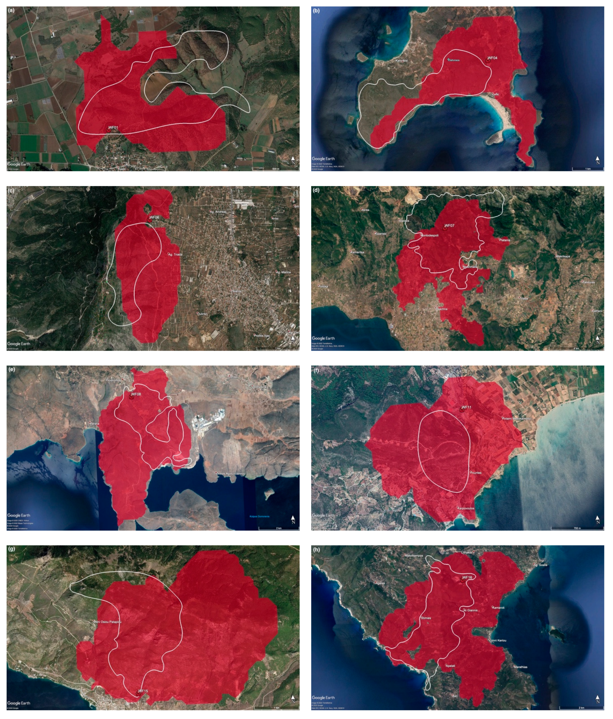
3.2. Wildfire Spread Forecasts

During the 2019 fire season, IRIS showed consistent performance in terms of reproducing wildfire spread. As summarized in Table 4, the model was able to predict the spatial extent of BAs better than random chance (p ≤ 0.10) in all examined events. KC and SC were computed to exceed the threshold value of 0.40, which indicates at least moderate agreement between the actual and predicted wildfire perimeters. The model performed best in the case of WF01, whereas the worst performance was seen in the case of WF15. The accuracy in wind simulation must have played a role in shaping this feature in the model’s performance since WF01 and WF15 are also the cases for which the model provided the overall best and worst wind forecasts, respectively (Table 3). Not surprisingly, BAs were overestimated (OI > 0) in all simulated wildfires. This can be attributed, at least to some extent, to the fact that tactical wildfire suppression activities are not taken into account.
Complementarily to the statistical evaluation (Table 2), the visual comparison between the actual and predicted wildfire perimeters (Figure 3) revealed interesting aspects of IRIS’s performance during the 2019 fire season. In all events, the actual and predicted BAs were found to overlap to a significant spatial extent. However, notable differences did exist. For instance, it could be clearly seen that IRIS was not able to capture the spatial extent of the southwest propagation of the wildfire front in WF04 (Figure 3b), which led to a BAU (220 ha) about half the size of the observed BA (535 ha). This BA underprediction, which was the largest in 2019, appears to coincide with the largest lag (~4 h) between the actual time of ignition and the activation time of IRIS (Table 1). Hence, it could be speculated that at least a part of this large underprediction could be attributed to neglecting a long period of active wildfire spread. Nevertheless, it should be noted that the wildfire spread was overpredicted to the southeast, indicating that the representation of wind conditions should have also played a role (Table 3). Poor representation of wind may also be the reason for the large unburnt areas seen in IRIS’s predictions for WF06 (Figure 3c), WF07 (Figure 3d), and WF15 (Figure 3g), for which the largest errors in wind direction were computed (Table 3).

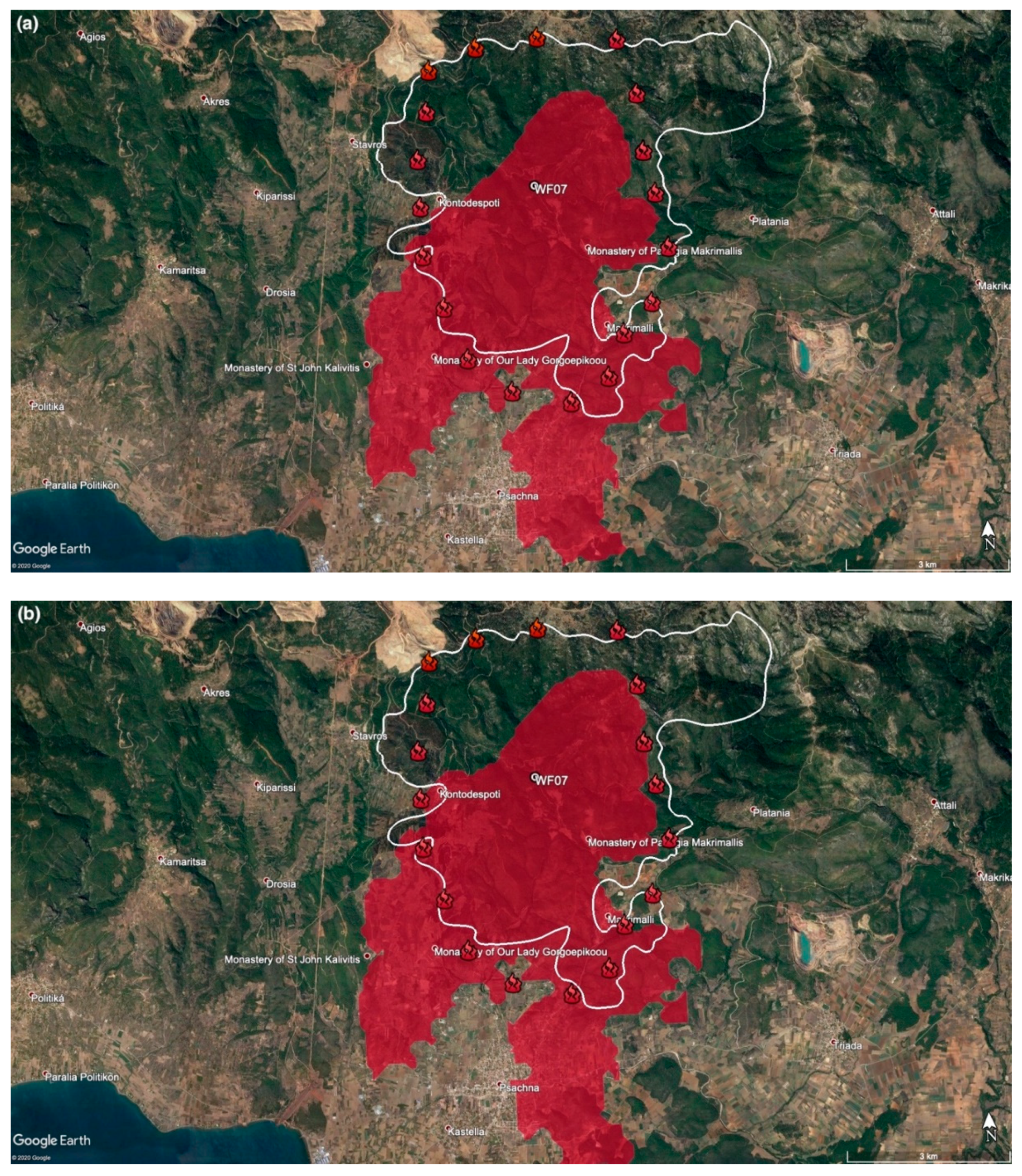
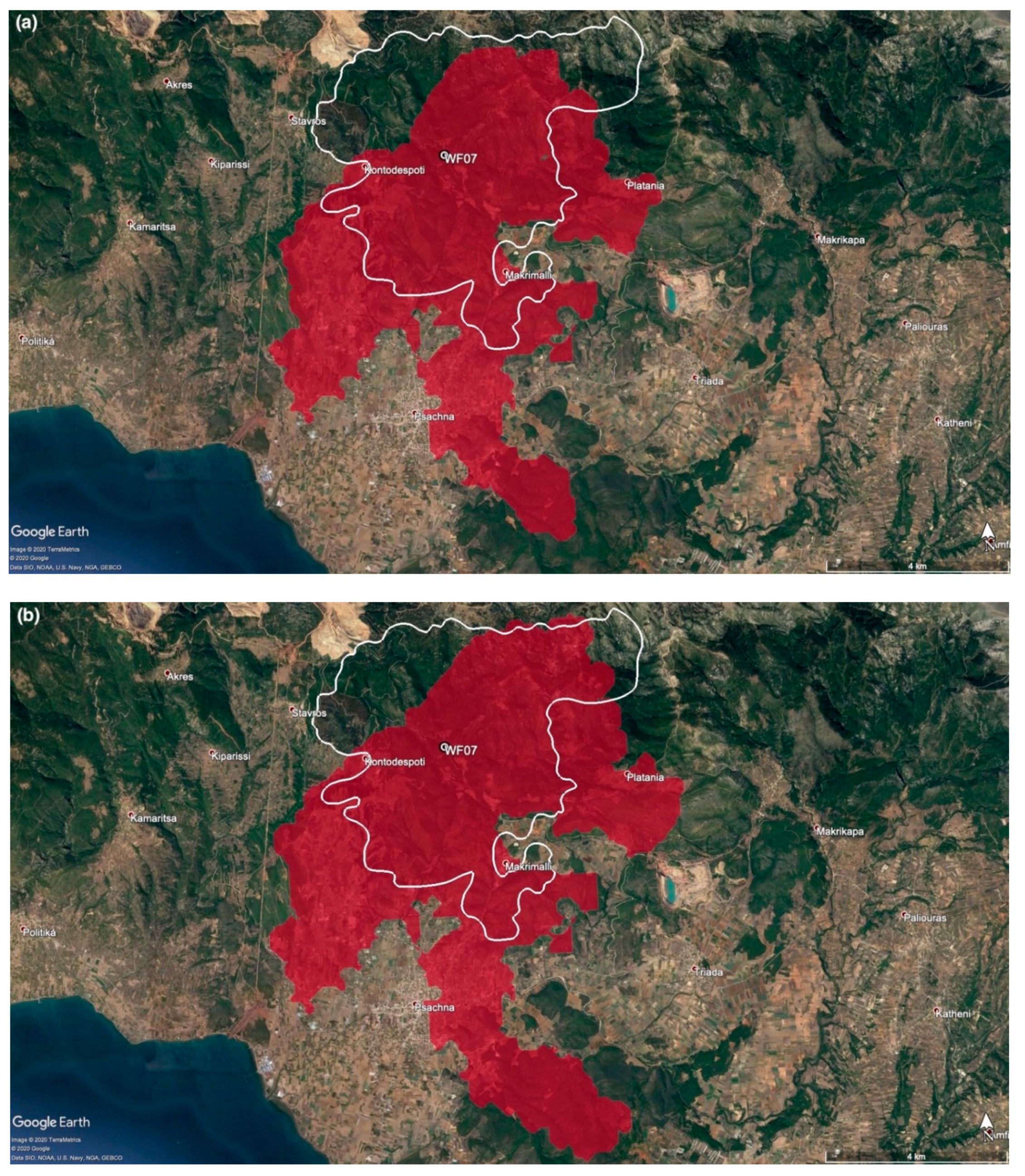
3.3. The Kontodespoti Wildfire (WF07)

The most significant and largest event of the 2019 fire season in Greece was the Kontodespoti wildfire (WF07; Table 1) in central Euboea. According to the HFC records, the wildfire broke out late in the night on 13 August, about 2 km east of the Kontodespoti village and 6 km north of the city of Psachna (Figure 3d), within a dense pine forest. The severity of the event was revealed early in the morning, when a convective plume could be clearly seen (Figure 4), indicating a plume-dominated wildfire. Such wildfires exhibit the increased role of the convective force generated by the heating of the burning fuels and tend to significantly influence the wind field in their vicinity. As a result, plume-dominated wildfires are commonly characterized by unpredictable behavior and are thus extremely difficult to contain.
The Kontodespoti wildfire was active for approximately 39 h, burning a total surface of nearly 3000 ha. However, according to the HFC, more than 2400 ha of land had already been burnt by the first 19 h of active wildfire spread. Figure 5a presents a visual comparison between the approximate location of the wildfire’s fronts and the corresponding IRIS prediction at 19:00 UTC on 13 August. Clearly, IRIS was able to predict most of the southward and eastward propagation of the wildfire. The overprediction of the BA to the south could be attributed to neglecting wildfire suppression activities and overestimating wind speed (Table 3). Indeed, the southward movement of the wildfire forced authorities and the HFC to set up emergency wildfire break zones in order to prevent further propagation of the wildfire towards the city of Psachna. On the other hand, it could also be seen that IRIS failed to capture the extent of wildfire spread to the northwest of the ignition location. Part of this underestimation could be attributed to the ~1 h time lag between the actual ignition time and the system’s activation time (Table 1). Other possible explanations could be associated with the uncertainty in defining the ignition location, the representation of fuels, the simulation of meteorological conditions, and the negligence of fire spotting. In particular, it must be noted that ignition coordinates are currently provided through the location of the firefighting crew that arrives first on-site. On certain occasions, this could lead to important differences between the real ignition location and the one provided during the activation of IRIS.
To investigate further the above-noted discrepancies and associated speculations, we conducted an additional, retrospective simulation of the Kontodespoti wildfire. Compared to its operational counterpart, the retrospective simulation was carried out using the actual ignition time of the wildfire instead of IRIS’s activation time (Table 1). Results suggest a slight improvement in model performance. As seen in Figure 5b, the consideration of the actual ignition time allowed for a more accurate prediction of the northeast propagation of the wildfire. However, it was not possible to resolve the major underestimation of BA to the northwest. This inadequacy of IRIS is still evident when examining the final observed and predicted wildfire perimeters (Figure 6). Indeed, while the retrospective prediction reproduced better the northeast propagation of the wildfire, it lacked the ability to predict propagation to the northwest. Further, it is worth noting that the consideration of the actual ignition time did not result in significant improvements in IRIS’s verification statistics (Table 5).
In considering the above results, it becomes quite clear that for the Kontodespoti wildfire, the highlighted underprediction of BA did not result from the difference between the actual ignition time and IRIS’s activation time. Moreover, the examination of both the operational and retrospective meteorological forecast (not shown) indicated minor differences in the model performance with respect to wind simulation. Additional numerical experiments (not shown), initializing the model with the ECMWF (European Center for Medium-range Weather Forecasts) operational surface and upper-air analysis and forecast data, did not improve IRIS’s wildfire spread prediction. Therefore, from an operational point of view, it can be claimed that it would be impossible to obtain a better prediction by only changing the initialization data of the model. One could argue that a better prediction could have been obtained by adopting a different model physics and/or domain setup. Such a claim is plausible, but its evaluation lies beyond the scope of our work.

4. Discussion and Conclusions

Coupled fire-atmosphere modeling systems are still not widely used in wildfire incident management. Instead, operational agencies and wildfire managers tend to rely on empirical and semi-empirical models that have proven to be able to provide reliable wildfire spread predictions [13,38,39,40]. However, such models neglect fire-atmosphere feedbacks that can be of great importance for the accurate simulation of wildfire spread. In this work, we aim to demonstrate that coupled fire-atmosphere modeling systems have great potential to be operationally employed in wildfire incident management. For this, we present the operational implementation and evaluation of such a forecasting system, which was specifically developed and used for providing rapid response support to the tactical wildfire suppression activities of the HFC in Greece.
Named IRIS, the presented forecasting system is based on the coupled fire-atmosphere WRF-Fire model [44]. The latter has been used in several past studies that focused primarily on simulating selected large wildfires [23,62,63,64]. While providing useful insights into the model performance, previous studies hardly included any quantitative assessment. More importantly, the consideration of single events does not allow for drawing a wider picture in terms of the capacity of the model to support operational activities. Our work differs significantly from such an approach, presenting and evaluating, both quantitatively and qualitatively, wildfire spread predictions that have been produced and used operationally during the 2019 fire season in Greece. To the best of our knowledge, this should be one of the first, if not the first, studies that introduce the performance evaluation of an operational rapid response fire spread forecasting system based on a coupled fire-atmosphere modeling system.
In a previous study, Giannaros et al. [24] showed that with proper adaptation, IRIS could be exploited for operationally supporting wildfire incident management. The present study confirms this preliminary conclusion. Our results, obtained through a quantitative verification of operational wildfire spread predictions for eight events, clearly highlight that IRIS is able to provide forecast guidance that is meaningful and useful to wildfire incident managers. In particular, the conducted accuracy assessment of the system’s predictions revealed an overall satisfactory performance (Table 2). Actual and predicted wildfire perimeters were found to be characterized by moderate agreement, with the model overestimating BAs in all examined events (Figure 3). As previously noted, this tendency of IRIS to overestimate BAs is not that surprising, considering that firefighting activities are neglected. Focusing on the largest event of the 2019 fire season, we also showed that IRIS was able to predict well enough the propagation of the wildfire (Figure 5).
Besides the positives of IRIS’s operational performance in 2019, one should also notice and discuss the negatives, in particular with respect to the further development and improvement of the system. Focusing on the largest event of the 2019 fire season, it was found that the consideration of the actual ignition time instead of IRIS’s activation time does improve wildfire spread prediction (Figure 5 and Figure 6). While this improvement may not always compensate for BA underprediction, it is important to be taken into account. IRIS was implemented operationally for the first time in 2019 and officers of the HFC needed time to familiarize themselves with its use and build experience on when to request its activation. Indeed, the time difference between the system’s activation and the actual ignition time was gradually reduced towards the end of the fire season (Table 1). Accounting for this, and based on the results of this work, it was decided that for the operational implementation of IRIS in 2020, the system’s activation time will be adjusted by 30 min; i.e., 30 min will be subtracted by the time of IRIS’s activation to better estimate the actual ignition time.
Other sources of uncertainty in IRIS’s predictions are related to the simulation of meteorological conditions and the representation of fuels and fuel moisture. Considering the former, our work has shown that special attention should be paid to properly simulate wind conditions. As for the representation of fuels, the prototype fuel map used by IRIS [24] is currently being updated and upgraded; new fuel models are being added and the horizontal resolution is being increased, so as to better represent spatial variability. Last but not least, the development of IRIS is continued by examining the inclusion of fire spotting and the online computation of fuel moisture, as well as by increasing the system’s spatial resolution in order to better capture the dynamic fire-atmosphere interactions.
In conclusion, the operational implementation of IRIS during the 2019 fire season in Greece and its subsequent performance evaluation revealed that coupled fire-atmosphere modeling systems do have great potential to support wildfire incident management. Our statement is not only supported by the results of this study, but also by the fact that IRIS’s activations almost doubled in 2020. IRIS was activated 17 times by the HFC in 2019, and 31 times during the ongoing 2020 fire season. As far as we can be aware, IRIS is currently the sole coupled fire-atmosphere modeling system implemented operationally within the European Union, and certainly one of the very few such operational systems implemented worldwide [23,28].

Author Contributions

Conceptualization, T.M.G.; methodology, T.M.G., V.K., K.L.; software, T.M.G.; validation, T.M.G.; formal analysis, T.M.G., V.K., K.L.; investigation, T.M.G., V.K., K.L.; resources, T.M.G., V.K., K.L.; data curation, T.M.G.; writing—original draft preparation, T.M.G.; writing—review and editing, V.K., K.L.; visualization, T.M.G.; supervision, V.K., K.L.; project administration, V.K.; funding acquisition, V.K. All authors have read and agreed to the published version of the manuscript.

Funding

This research was co-funded by the European Union (European Research Development Fund & Instrument for Pre-accession Assistance) and National Funds, under the INTERREG Balkan-Mediterranean 2014 –2020 cooperation programme (project DISARM), and by the flagship initiative National Network on Climate Change (CLIMPACT), financed by the General Secretariat for Research and Technology (GRST) of Greece.

Acknowledgments

The authors would like to acknowledge the role of the Hellenic Fire Corps in motivating the development and implementation of IRIS. Special acknowledgments must be addressed specifically to Lieutenant Colonels Markos Gkouvas and Zisoula Dasiou for their close collaboration and invaluable feedback. The authors would also like to acknowledge NCEP for freely providing the operational data required for the implementation of IRIS at an operational basis.

Conflicts of Interest

The authors declare no conflict of interest. The funders had no role in the design of the study; in the collection, analyses, or interpretation of data; in the writing of the manuscript, or in the decision to publish the results.

References

  1. Bond, W.J.; Woodward, F.I.; Midgley, G.F. The global distribution of ecosystems in a world without fire. New Phytol. 2005, 165, 525–538. [Google Scholar] [CrossRef] [PubMed]
  2. Pausas, J.G.; Vallejo, V.R. The role of fire in European Mediterranean ecosystems. In Remote Sensing of Large Wildfires; Chuvieco, E., Ed.; Springer: Berlin/Heidelberg, Germany, 1999; pp. 3–16. [Google Scholar]
  3. San-Miguel-Ayanz, J.; Durrant, T.; Boca, R.; Liberta, G.; Branco, A.; de Rigo, D.; Ferrari, D.; Maianti, P.; Artes Vivancos, T.; Pfeiffer, H.; et al. Forest Fires in Europe, Middle East and North Africa 2018; Publications Office of the European Union: Luxembourg, 2018; pp. 1–178. [Google Scholar]
  4. San-Miguel-Ayanz, J.; Camia, A. Forest fires. In Mapping the Impacts of Natural Hazards and Technological Accidents in Europe. An Overview of the Last Decade; Wehrli, A., Herkendell, J., Jol, A., Eds.; European Environment Agency: Copenhagen, Denmark, 2010; pp. 47–53. [Google Scholar]
  5. Molina-Terrén, D.M.; Xanthopoulos, G.; Diakakis, M.; Ribeiro, L.; Caballero, D.; Delogu, G.M.; Viega, D.X.; Silva, C.A.; Cardil, A. Analysis of forest fire fatalities in souther Europe: Spain, Portugal, Greece and Sardinia (Italy). Int. J. Wildland Fire 2019, 28, 85–98. [Google Scholar] [CrossRef] [Green Version]
  6. Shakesby, R.A. Post-wildfire soil erosion in the Mediterranean: Review and future research directions. Earth Sci. Rev. 2011, 105, 71–100. [Google Scholar] [CrossRef]
  7. San-Miguel-Ayanz, J.; Moreno, J.M.; Camia, A. Analysis of large fires in European Mediterranean landscapes: Lessons learned and perspectives. Forest Ecol. Manag. 2013, 294, 11–22. [Google Scholar] [CrossRef]
  8. European Commission. Forest Fires in Europe 2003 Fire Campaign; European Commission: Brussels, Belgium, 2004; pp. 6–10. [Google Scholar]
  9. Lagouvardos, K.; Kotroni, V.; Giannaros, T.M.; Dafis, S. Meteorological conditions conducive to the rapid spread of the deadly wildfire in Eastern Attica, Greece. Bull. Am. Meteorol. Soc. 2019, 100, 2137–2145. [Google Scholar] [CrossRef]
  10. Flannigan, M.D.; Krawchuk, M.A.; de Groot, W.J.; Wotton, B.M.; Gowman, L.M. Implications of changing climate for global wildland fire. Int. J. Wildland Fire 2009, 18, 483–507. [Google Scholar] [CrossRef]
  11. Ganteaume, A.; Camia, A.; Jappiot, M.; San-Miguel-Ayanz, J.; Long-Fournel, M.; Lampin, C. A review of the main driving factors of forest fire ignition over Europe. Environ. Manag. 2013, 51, 651–662. [Google Scholar] [CrossRef] [Green Version]
  12. Andrews, P.; Finney, M.; Fischetti, M. Predicting wildfires. Sci. Am. 2007, 297, 46–55. [Google Scholar] [CrossRef]
  13. Arca, B.; Ghisu, T.; Casula, M.; Salis, M.; Duce, P. A web-based wildfire simulator for operational applications. Int. J. Wildland Fire 2019, 28, 99–112. [Google Scholar] [CrossRef]
  14. Coen, J. Some requirements for simulating wildland fire behavior using insight from coupled weather—Wildland fire models. Fire 2018, 1, 6. [Google Scholar] [CrossRef] [Green Version]
  15. Linn, R.; Reisner, J.; Colman, J.J.; Winterkamp, J. Studying wildfire behavior using FIRETEC. Int. J. Wildland Fire 2002, 11, 233–246. [Google Scholar] [CrossRef]
  16. Mell, W.; Jenkins, M.A.; Gould, J.; Cheney, P. A physics-based approach to modeling grassland fires. Int. J. Wildland Fire 2007, 16, 1–22. [Google Scholar] [CrossRef]
  17. Finney, M.A. FARSITE: Fire Area Simulator—Model Development and Evaluation; US Forest Service: Ogden, UT, USA, 1998.
  18. Andrews, P.L. BehavePlus fire modeling system: Past, present and future. In Proceedings of the 7th Symposium on Fire and Forest Meteorology, Bar Harbor, ME, USA, 23–25 October 2007. Paper J2.1. [Google Scholar]
  19. Papadopoulos, G.D.; Pavlidou, F.N. A comparative review of wildfire simulators. Syst. J. IEEE 2011, 5, 233–243. [Google Scholar] [CrossRef]
  20. Sullivan, A.L. Wildland surface fire spread modeling, 1990–2007. 1: Physical and quasi-physical models. Int. J. Wildland Fire 2009, 18, 349–368. [Google Scholar] [CrossRef] [Green Version]
  21. Cruz, M.G.; Alexander, M.E. Uncertainty associated with model predictions of surface and crown fire rates of spread. Environ. Model. Softw. 2013, 47, 16–28. [Google Scholar] [CrossRef]
  22. Filippi, J.-B.; Bosseur, F.; Mari, C.; Lac, C. Simulation of a large wildfire in a coupled fire-atmosphere model. Atmosphere 2018, 9, 218. [Google Scholar] [CrossRef] [Green Version]
  23. Jiménez, P.A.; Muñoz-Esparza, G.; Kosović, B. A high resolution coupled fire-atmosphere forecasting system to minimize the impacts of wildland fires: Applications to the Chimney Tops II wildland event. Atmosphere 2018, 9, 197. [Google Scholar] [CrossRef] [Green Version]
  24. Giannaros, T.M.; Kotroni, V.; Lagouvardos, K. IRIS—Rapid response fire spread forecasting system: Development, calibration and evaluation. Agric. Forest Meteorol. 2019, 279, 107745. [Google Scholar] [CrossRef]
  25. Coen, J.L. Simulation of the Big Elk fire using coupled atmosphere-fire modeling. Int. J. Wildland Fire 2005, 14, 49–59. [Google Scholar] [CrossRef]
  26. Filippi, J.-B.; Pialat, X.; Clements, C.B. Assessment of Forefire/Meso-NH for wildland fire/atmosphere coupled simulation of the FireFlux experiment. Proc. Combust. Inst. 2013, 34, 2633–2640. [Google Scholar] [CrossRef]
  27. Kochanski, A.K.; Jenkins, M.A.; Mandel, J.; Beezley, J.D.; Clements, C.B.; Krueger, S. Evaluation of WRF-SFIRE performance with field observations from the Fireflux experiment. Geosci. Model Dev. 2013, 6, 1109–1126. [Google Scholar] [CrossRef] [Green Version]
  28. Kochanski, A.K.; Jenkins, M.A.; Mandel, J.; Beezley, J.D.; Krueger, S. Real time simulation of 2007 Santa Ana fires. Forest Ecol. Manag. 2013, 294, 136–149. [Google Scholar] [CrossRef] [Green Version]
  29. Peace, M.; Mattner, T.; Mills, G.; Keppert, J.; McCaw, L. Coupled fire-atmosphere simulations of the Rocky River fire using WRF-SFIRE. J. Appl. Meteorol. Climatol. 2016, 55, 1151–1168. [Google Scholar] [CrossRef]
  30. Toivanen, J.; Engle, C.B.; Reeder, M.J.; Lane, T.P.; Davies, L.; Webster, S.; Wales, S. Coupled atmosphere-fire simulations of the Black Saturday Kilmore East wildfires with the Unified Model. J. Adv. Model. Earth Syst. 2019, 11, 210–230. [Google Scholar] [CrossRef] [Green Version]
  31. Mallia, D.V.; Kochanski, A.K.; Kelly, K.E.; Whitaker, R.; Xing, W.; Mitchell, L.E.; Jacques, A.; Farguell, A.; Mandel, A.; Gaillardon, P.-E.; et al. Evaluating wildfire smoke transport within a coupled fire-atmosphere model using a high-density observation network for an episodic smoke event along Utah’s Wasatch Front. J. Geophys. Res. 2020, 125, e2020JD032712. [Google Scholar] [CrossRef]
  32. Mallia, D.V.; Kochanski, A.K.; Urbanski, S.P.; Mandel, J.; Farguell, A.; Krueger, S.K. Incorporating a canopy parameterization within a coupled fire-atmosphere model to improve smoke simulation for a prescribed burn. Atmosphere 2020, 11, 832. [Google Scholar] [CrossRef]
  33. Kochanski, A.K.; Mallia, D.V.; Fearon, M.G.; Mandel, J.; Souri, A.H.; Brown, T. Modeling wildfire smoke feedback mechanisms using a coupled fire-atmosphere model with a radiatively active aerosol scheme. J. Geophys. Res. 2019, 124, 9099–9116. [Google Scholar] [CrossRef]
  34. Clark, T.L.; Jenkins, M.A.; Coen, J.; Packham, D. A coupled atmosphere-fire model: Role of the convective Froude number and dynamic fingering at the fireline. Int. J. Wildland Fire 1996, 6, 177–190. [Google Scholar] [CrossRef] [Green Version]
  35. Simpson, C.C.; Sharples, J.J.; Evans, J.P. Resolving vorticity-driven lateral fire spread using the WRF-Fire coupled atmosphere-fire numerical model. Nat. Hazards Earth Syst. Sci. 2014, 14, 2359–2371. [Google Scholar] [CrossRef] [Green Version]
  36. Peace, M.; Mattner, T.; Mills, G.; Keppert, J.; McCaw, L. Fire-modified meteorology in a coupled fire-atmosphere model. J. Appl. Meteorol. Climatol. 2015, 54, 704–720. [Google Scholar] [CrossRef]
  37. Filippi, J.-B.; Bosseur, F.; Pialat, X.; Santoni, P.A.; Strada, S.; Mari, C. Simulation of coupled fire/atmosphere interaction with the MesoNH-ForeFire models. J. Combust. 2011, 2011, 540390. [Google Scholar] [CrossRef] [Green Version]
  38. Finney, M.A.; Grenfell, I.C.; McHugh, C.W.; Seli, R.C.; Trethewey, D.; Stratton, R.D.; Brittain, S. A method for ensemble wildland fire simulation. Environ. Model. Assess. 2011, 16, 153–167. [Google Scholar] [CrossRef]
  39. Kalabokidis, K.; Athanasis, N.; Gagliardi, F.; Karayiannis, F.; Palaiologou, P.; Parastatidis, S.; Vasilakos, C. Virtual fire: A web-based GIS platform for forest fire control. Ecol. Inform. 2013, 16, 62–69. [Google Scholar] [CrossRef]
  40. Salis, M.; Arca, B.; Alcasena, F.; Arianoutsou, M.; Bacciu, V.; Duce, P.; Duguy, B.; Koutsias, N.; Mallinis, G.; Mitsopoulos, I.; et al. Predicting wildfire spread and behavior in Mediterranean landscapes. Int. J. Wildland Fire 2016, 25, 1015–1032. [Google Scholar] [CrossRef]
  41. Forthofer, J.M.; Butler, B.W.; Wagenbrener, N.S. A comparison of three approaches for simulating fine-scale surface winds in support of wildland fire management. Part I. Model formulation and comparison against measurements. Int. J. Wildland Fire 2014, 23, 969–981. [Google Scholar] [CrossRef]
  42. Forthofer, J.M.; Butler, B.W.; McHugh, C.W.; Finney, M.A.; Bradshaw, L.S.; Stratton, R.D.; Shannon, K.S.; Wagenbrenner, N.S. A comparison of three approaches for simulating fine-scale surface winds in support of wildland fire management. Part II. An exploratory study of the effect of simulated winds on fire growth simulations. Int. J. Wildland Fire 2014, 23, 982–994. [Google Scholar] [CrossRef]
  43. Kotroni, V.; Cartalis, C.; Michaelides, S.; Stoyanova, J.; Tymvios, F.; Bezes, A.; Christoudias, T.; Dafis, S.; Giannakopoulos, C.; Giannaros, T.M.; et al. DISARM early warning system for wildfires in the eastern Mediterranean. Sustainability 2020, 12, 6670. [Google Scholar] [CrossRef]
  44. Muñoz-Esparza, D.; Kosović, B.; Jiménez, P.A.; Coen, J.L. An accurate fire-spread algorithm in the Weather Research and Forecasting model using the level-set method. J. Adv. Model. Earth Syst. 2018, 10, 908–926. [Google Scholar] [CrossRef] [Green Version]
  45. Dimitrakopoulos, A.P. Mediterranean fuel models and potential fire behavior in Greece. Int. J. Wildland Fire 2002, 11, 127–130. [Google Scholar] [CrossRef]
  46. Papagiannaki, K.; Giannaros, T.M.; Lykoydis, S.; Kotroni, V.; Lagouvardos, K. Weather-related thresholds for wildfire danger in a Mediterranean region: The case of Greece. Agric. Forest Meteorol. 2020, 291, 108076. [Google Scholar] [CrossRef]
  47. Hellenic Fire Corps. Available online: https://www.fireservice.gr/el_GR/synola-dedomenon (accessed on 26 August 2020).
  48. San-Miguel-Ayanz, J.; Schulte, E.; Schmuck, G.; Camia, A.; Srobl, P.; Libertà, G.; Giovando, C.; Boca, R.; Sedano, F.; Kempeneers, P.; et al. Comprehensive monitoring of wildfires in Europe: The European Forest Fire Information System (EFFIS). In Approaches to Monitor Disaster—Assessing Hazards, Emergencies and Disaster Impacts; Tiefenbacher, J.P., Ed.; InTechOpen: London, UK, 2012; pp. 87–105. [Google Scholar]
  49. Lagouvardos, K.; Kotroni, V.; Bezes, A.; Koletsis, I.; Kopania, T.; Lykoudis, S.; Mazarakis, N.; Papagiannaki, K.; Vougioukas, S. The automatic weather stations NOANN network of the National Observatory of Athens: Operation and database. Geosci. Data J. 2017, 4, 4–16. [Google Scholar] [CrossRef]
  50. Rothermel, R.C. A Mathematical Model for Predicting Fire Spread in Wildland Fuels; USDA Forest Service: Ogden, UT, USA, 1972.
  51. Coen, J.L.; Cameron, M.; Michalakes, J.; Patton, E.G.; Riggan, P.J.; Yedinak, K.M. WRF-Fire: Coupled weather-wildland fire modeling with the Weather Research and Forecasting model. J. Appl. Meteorol. Climatol. 2013, 52, 16–38. [Google Scholar] [CrossRef]
  52. Skamarock, W.C.; Klemp, J.B.; Dudhia, J.; Gill, D.O.; Liu, Z.; Berner, J.; Wang, W.; Powers, J.G.; Duda, M.G.; Barker, D.M.; et al. A Description of the Advanced Research WRF Model Version 4; National Center for Atmospheric Research (NCAR): Boulder, CO, USA, 2019. [Google Scholar]
  53. Iacono, M.G.; Delamere, J.S.; Mlawer, E.J.; Shephard, M.W.; Clough, S.A.; Collins, W.D. Radiative forcing by long-lived greenhouse gases: Calculations with the AER radiative transfer models. J. Geophys. Res. 2008, 113. [Google Scholar] [CrossRef]
  54. Thompson, G.; Field, P.R.; Rasmusse, R.M.; Hall, W.D. Explicit forecasts of winter precipitation using an improved bulk microphysics scheme. Part II: Implementation of a new snow parameterization. Mon. Weather Rev. 2008, 136, 5095–5115. [Google Scholar] [CrossRef]
  55. Hong, S.Y.; Noh, Y.; Dudhia, J. A new vertical diffusion package with an explicit treatment of entrainment processes. Mon. Weather Rev. 2006, 134, 2318–2341. [Google Scholar] [CrossRef] [Green Version]
  56. Jiménez, P.A.; Dudhia, J.; Gonzalerz-Rouco, J.F.; Navarro, J.; Montavez, J.P.; Garcia-Bustamante, E. A revised scheme for the WRF surface layer formulation. Mon. Weather Rev. 2012, 140, 898–918. [Google Scholar] [CrossRef] [Green Version]
  57. Tewari, M.; Chen, F.; Wang, W.; Dudhia, J.; LeMone, M.A.; Mitchell, K.; Ek, M.; Gayno, G.; Wegiel, J.; Cuenca, R.H. Implementation and verification of the unified NOAH land surface model in the WRF model. In Proceedings of the 20th Conference on Weather Analysis and Forecasting/16th Conference on Numerical Weather Prediction, Seattle, Washington, DC, USA, 12–16 January 2004; pp. 11–15. [Google Scholar]
  58. Grell, G.A.; Freitas, S.R. A scale and aerosol aware stochastic convective parameterization for weather and air quality modeling. Atmos. Chem. Phys. 2014, 14, 5233–5250. [Google Scholar] [CrossRef] [Green Version]
  59. Jarvis, A.; Reuter, H.I.; Nelson, A.; Guevara, E. Available online: http://srtm.csi.cgiar.org (accessed on 4 September 2020).
  60. Congalton, R.G. A review of assessing the accuracy of classifications of remotely sensed data. Remote Sens. Environ. 1991, 37, 35–46. [Google Scholar] [CrossRef]
  61. Sorensen, T.A. A method of establishing groups of equal amplitude in plant sociology based on similarity of species content, and its application to analysis of the vegetation of Danish commons. K. Dan. Vidensk. Selsk. 1948, 5, 1–34. [Google Scholar]
  62. Coen, J.L.; Riggan, P.J. Simulation and thermal imaging of the 2006 Esperanza wildfire in southern California: Application of a coupled weather-wildland fire model. Int. J. Wildland Fire 2014, 23, 755–770. [Google Scholar] [CrossRef]
  63. Coen, J.L.; Schroeder, W. The high park fire: Coupled weather-wildland fire model simulation of a windstorm-driven wildfire in Colorado’s front range. J. Geophys. Res. Atmos. 2015, 120, 131–146. [Google Scholar] [CrossRef]
  64. Coen, J.L.; Stavros, E.N.; Fites-Kaufmann, J.A. Deconstructing the King megafire. Ecol. Appl. 2018, 28, 1565–1580. [Google Scholar] [CrossRef] [PubMed]
Figure 1. Locations of the 17 wildfires for which IRIS was activated during the 2019 fire season in Greece.
Atmosphere 11 01264 g001
Figure 2. Flow chart of the IRIS rapid response fire spread forecasting system.
Atmosphere 11 01264 g002
Figure 3. Visual comparison between actual (white contours) and predicted (red shades) wildfire perimeters for the selected events of the 2019 fire season in Greece: (a) WF01, (b) WF04, (c) WF06, (d) WF07, (e) WF08, (f) WF11, (g) WF15, and (h) WF16.
Atmosphere 11 01264 g003
Figure 4. Aspects of the convective plume of the Kontodespoti wildfire at 05:43 UTC on 13 August 2019, as seen from onboard a commercial flight. (Photographs courtesy of Fotis Fillipopoulos, Twitter: @F_Fillipopoulos).
Atmosphere 11 01264 g004
Figure 5. Visual comparison between the approximate location of the wildfire’s fronts (red flames) and IRIS’s prediction at 19:00 UTC on 13 August. The black dot (WF07) denotes the provided ignition location. White contours denote the actual final wildfire perimeter. (a) Operational wildfire spread prediction based on IRIS’s activation time, and (b) Retrospective wildfire spread prediction based on actual ignition time.
Atmosphere 11 01264 g005
Figure 6. Visual comparison between actual (white contour) and predicted (red shades) wildfire perimeters for the Kontdespoti wildfire (WF07). (a) Operational wildfire spread prediction based on IRIS’s activation time, and (b) Retrospective wildfire spread prediction based on actual ignition time.
Atmosphere 11 01264 g006
Table 1. Summary of the eight most significant wildfires of the 2019 fire season in Greece, for which IRIS was activated by the Hellenic Fire Corps (HFC) and provided spread predictions. The “Date and Time (UTC)” column reports the actual time of wildfire ignition according to the official records of the HFC [47]. The “IRIS activation (UTC)” column reports the time of system activation by HFC officers (Section 2.2).
IDRegionDate and Time (UTC)IRIS Activation (UTC)Location
(°N, °E)
Duration
(hh: mm)
BA (ha)Perimeter Acquisition Date
WF01Kastri8 July 2019
11:37
8 July 2019
12:40
38.94925,
22.20243
09:23988 July 2019
WF04Elafonissos10 August 2019
02:40
10 August 2019
06:56
36.48591,
22.97353
38:2053511 August 2019
WF06Hymettus12 August 2019
00:19
12 August 2019
01:20
37.97047,
23.83132
06:4118012 August 2019
WF07Kontodespoti13 August 2019
00:10
13 August 2019
01:25
38.62776,
23.65245
38:50288915 August 2019
WF08Prodromos13 August 2019
02:35
13 August 2019
03:40
38.24905,
22.91353
12:2573513 August 2019
WF11Mesokampos24 August 2019
14:09
24 August 2019
14:48
37.70667,
26.96484
14:515926 August 2019
WF15Loutraki14 September 2019
12:36
14 September 2019
13:27
37.98038,
22.98734
20:2435216 September 2019
WF16Lithakia15 September 2019
08:00
15 September 2019
08:32
37.70666,
20.82235
22:3091916 September 2019
Table 2. Summary of the automatic weather stations (AWSs) used for the evaluation of IRIS’s wind predictions.
IDStationLatitude
(°N)
Longitude
(°E)
Verification Period
(UTC)
Comments
WF01Makrakomi38.937522.11688 July 2019 13:00–
8 July 2019 21:00
7.5 km WSW of ignition location
WF04Kavomalias36.475823.101210 August 2019 07:00–
11 August 2019 06:00
11 km ESE of ignition location
WF06Palini37.997823.892812 August 2019 02:00–
12 August 2019 07:00
6 km NE of ignition location
WF07Psachna38.569423.649213 August 2019 02:00–
14 August 2019 03:00
6.4 km S of ignition location
WF08Kapareli38.243323.211713 August 2019 04:00–
13 August 2019 15:00
26.5 km E of ignition location
WF11Samos37.793726.682024 August 2019 15:00–
25 August 2019 05:00
26 km NW of ignition location
WF15Loutraki37.969622.979914 September 2019 14:00–
15 September 2019 09:00
1.4 km SSW of ignition location
WF16Zakynthos37.781020.845015 September 2019 09:00–
16 September 2019 07:00
8.4 km NNE of ignition location
Table 3. Statistical evaluation of IRIS’s wind speed and direction forecasts during the 2019 fire season. Note that for WF11, the evaluation could not be conducted due to the unavailability of valid observed data (i.e., all wind measurements failed to pass the threshold value of 2 m s−1; Section 2.3).
Wind Speed (m s−1)Wind Direction (°)
IDMERMSEMERMSE
WF010.50.72.418.9
WF040.51.729.136.8
WF061.72.3−52.9136.6
WF071.02.519.461.5
WF082.62.741.552.1
WF11n/an/an/an/a
WF151.63.030.2103.7
WF161.61.744.749.8
Table 4. Statistical evaluation of IRIS’ wildfire spread forecasts during the 2019 fire season in Greece. Values of KC followed by * denote statistical significance (Z-test) at p ≤ 0.10.
IDKCSCOIBAA (ha) 1BAO (ha) 2BAU (ha) 3
WF010.63 *0.680.44755220
WF040.45 *0.490.06268298266
WF060.45 *0.480.4511418068
WF070.52 *0.570.3218991908989
WF080.57 *0.600.9370290935
WF110.49 *0.520.96571042
WF150.42 *0.460.7928360471
WF160.52 *0.550.848141217103
1 Burnt area agreement 2 Burnt area overestimation 3 Burnt area underestimation.
Table 5. Statistical evaluation of IRIS’s operational and retrospective wildfire spread predictions for the Kontodespoti wildfire (WF07). Values of KC followed by * denote statistical significance (Z-test) at p ≤ 0.10.
IDKCSCOIBAA (ha) 1BAO (ha) 2BAU (ha) 3
Operational Prediction
WF070.52 *0.570.3218991908989
Retrospective Prediction
WF070.52 *0.570.4921012288787
1 Burnt area agreement 2 Burnt area overestimation 3 Burnt area underestimation.
Publisher’s Note: MDPI stays neutral with regard to jurisdictional claims in published maps and institutional affiliations.

