A Simulation Experiment to Retrieve the Atmospheric Density and Three-Dimensional Wind Field by Double Falling Spheres

Abstract

Falling-sphere sounding remains an important method for in situ determination in the middle atmosphere and is the only determination method within the altitude range of 60–100 km. Traditional single-falling-sphere sounding indicates only the atmospheric density and horizontal wind but not the vertical wind; the fundamental reason is that the equation set for retrieving atmospheric parameters is underdetermined. For tractability, previous studies assumed the vertical wind, which is much smaller than the horizontal wind, to be small or zero. Obtaining vertical wind profiles necessitates making the equations positive definite or overdetermined. An overdetermined equation set consisting of six equations, by which the optimal solution of density and three-dimensional wind can be obtained, can be established by the double-falling-sphere method. Hence, a simulation experiment is designed to retrieve the atmospheric density and three-dimensional wind field by double falling spheres. In the inversion results of the simulation experiment, the retrieved density is consistent with the constructed atmospheric density in magnitude; the density deviation rate does not generally exceed 20% (less than 5% below 60 km). The atmospheric density retrieved by the double-falling-sphere method is more accurate at low altitudes than the single-falling-sphere method. The vertical wind below 50 km and horizontal wind retrieved by double-falling-sphere method is highly consistent with the constructed average wind field. Additionally, the wind field deviation formula is deduced. These results establish the fact that the double-falling-sphere method is effective in detecting atmospheric density and three-dimensional wind.

1. Introduction

The middle atmosphere, which refers to the region extending from more than 10 km to approximately 100 km above the ground, includes the stratosphere, the mesosphere and the lower thermosphere [1,2]. In recent years, numerous studies of this thin and neutral atmosphere have been carried out [3]. He et al. [4] explored the spectral characteristics of temperature fluctuations and three-dimensional wind field fluctuations by a set of near-space high-resolution balloon data and increased the height range of spectral analysis to 38 km. He et al. [5] analyzed the scale interactions between the small-scale gravity wave and turbulence in the middle stratosphere. Sheng et al. [6] applied Thorpe analysis to COSMIC (Constellation Observing System for Meteorology, Ionosphere, and Climate) data to retrieve the strongest mixed layer in the troposphere (SMLT) altitude.

Wind is one of the key parameters of atmospheric dynamics [7]. The neutral wind field not only plays an important role in the energy transmission and atmospheric dynamics but also has a great impact on the safety and orbits of spacecraft along with atmospheric density and temperature [8]. The understanding of the middle atmospheric wind field is of great significance to the study of dynamics and behaviors of the middle atmosphere and the development of forecasting capabilities for weather and space environments [9]. However, there are still few measurement methods for the wind field of the middle atmosphere at present. During the past decade, horizontal winds have been measured from space for the first time from 30 to 90 km using submillimetric limb sounding, and the Swedish Space Agency will launch the Stratospheric Inferred Winds (SIW) satellite in 2023 [10]. Baron et al. [10] conducted a simulation study to assess the measurement performance of SIW. Additionally, the main passive optical instruments used for neutral wind measurement include the Fabry-Perot interferometer [11], Michelson interferometer [12] and Doppler asymmetric spatial heterodyne spectrometer interferograms [13]. Using meteor radar [14], lidar [15,16], medium frequency radar [17], etc. can also measure atmospheric parameters such as the wind field in the middle atmosphere. The measurement methods mentioned above are all remote sensing methods, but in situ measurement methods are still necessary for small-scale or short-term middle atmosphere study.

The falling sphere sounding method is an important measurement method for the middle atmospheric parameters and the only in situ measurement method at altitudes ranging from 60 to 100 km [18,19]. Bartman et al. [20] used the trajectory data of an inflatable sphere with a small antenna and a transponder to retrieve the atmospheric density and temperature profiles successfully. Otterman et al. [21] described the theory of using the falling sphere to retrieve the upper atmosphere density and horizontal wind field. Faucher et al. [22] obtained atmospheric density, pressure and temperature profiles over 88–128 km using an inflatable sphere carrying a tri-axial accelerometer. Yuan et al. [23] obtained atmospheric density, temperature and horizontal wind field profiles by GPS data from rigid falling spheres. Ge et al. [24] used the radar tracking data of the first passive falling sphere experiment in China’s northwest region to retrieve the horizontal wind field and extracted wind shear and gravity waves from the horizontal wind field.

In previous studies using falling spheres to retrieve atmospheric parameters, vertical wind is usually ignored [20,25] or assumed to be a small value [23,26] since it is very small compared with horizontal wind and difficult to measure [27]. Although this can ensure the completeness of the equations for retrieving atmospheric parameters, it also introduces new errors at the same time.

The vertical wind field plays a significant role in the vertical transport of momentum, kinetic energy and gravity potential energy [27]. However, few previous studies have discussed the specific methods of obtaining vertical wind using the falling sphere. Jones and Peterson [28] mentioned that vertical wind might be measured by the trajectories of two spheres with different mass-to-area ratios, but to date, no study or experiment on the inversion of vertical wind with double falling spheres has been conducted. Therefore, in this paper, the theory of the double-falling-sphere method is described in detail, a simulation experiment using double falling spheres to retrieve the three-dimensional wind field and atmospheric density is designed to verify the feasibility of this method, and the error of the retrieved three-dimensional wind field is discussed.

In this paper, Section 2 introduces the data used in the simulation experiment of retrieving the atmospheric density and three-dimensional wind field by double falling spheres. Section 3 describes the theory and experimental design of calculating the three-dimensional wind field using double falling spheres, and the inversion results are given in Section 4. The causes and formula of wind field deviation are discussed in detail in Section 5. Finally, our conclusions are given in Section 6.

2. Data

The neutral atmospheric density and temperature profile data provided by the NRLMSISE-00 (NRL: US Naval Research Laboratory, MSIS: Mass Spectrometer and Incoherent Scatter radar, E: Exosphere) model are used as the simulated reference atmospheric density and temperature. The three-dimensional average wind field of the atmosphere required for the simulation experiment is constructed based on the atmospheric horizontal wind profile data provided by the Modern-Era Retrospective Analysis for Research and Applications, version 2 (MERRA-2).

2.1. NRLMSISE-00 Model

The NRLMSISE-00 atmosphere model, which is currently one of the most widely used atmospheric models, can provide physical quantities such as neutral atmospheric density and temperature for the region from 0 to 1000 km [29]. This paper uses the neutral atmospheric density and temperature profile data provided by the NRLMSISE-00 model as the simulated reference atmospheric density and temperature. Additionally, the upper atmosphere temperature of the model is used as the initial atmosphere temperature in the inversion process.

2.2. MERRA-2 Atmospheric Reanalysis Data Set

MERRA-2 is a global atmospheric reanalysis dataset that includes various meteorological parameters, such as net radiation, temperature, relative humidity, and wind speed. In this paper, the wind field data of MERRA-2 are used as the simulated horizontal wind field from 20 to 60 km.

3. Double-Falling-Sphere Measurement Method

3.1. Theory

A single sphere is mainly affected by the combined action of gravity, buoyancy, the Coriolis force, and atmospheric drag during the falling process [16,22,24], which can be expressed as

$$\stackrel{\rightharpoonup }{a}=\stackrel{\rightharpoonup }{g}+\stackrel{\rightharpoonup }{a_b}+\stackrel{\rightharpoonup }{a_c}+\stackrel{\rightharpoonup }{a_d},$$

(1)

where $\stackrel{\rightharpoonup }{a}$ is the total acceleration of the falling sphere, $\stackrel{\rightharpoonup }{g}$ is the acceleration of gravity, $\stackrel{\rightharpoonup }{a_b}$ is the acceleration of buoyancy, $\stackrel{\rightharpoonup }{a_c}$ is the acceleration of Coriolis force, and $\stackrel{\rightharpoonup }{a_d}$ is the acceleration of atmospheric drag.

The most important item in Equation (1) for retrieving the atmospheric wind field is the drag acceleration term, which can be expressed as

$$\stackrel{\rightharpoonup }{a_d}= -\frac{\rho A{C}_d\left|\stackrel{\rightharpoonup }{v_r}\right|\stackrel{\rightharpoonup }{v_r}}{2m},$$

(2)

where $\rho$ is the atmospheric density, $m$ is the mass of the sphere, $A$ is the cross-sectional area of the sphere, $\stackrel{\rightharpoonup }{v_r}$ is the velocity of the sphere relative to air (airspeed), which equals the ground speed ($\stackrel{\rightharpoonup }{v}$) minus the wind speed ($\stackrel{\rightharpoonup }{w}$), and $C_d$ is the drag coefficient. The drag coefficient is related to the Reynolds number and Mach number [20], that is, $C_d$ = $C_d\left(R_e,M_a\right)$. In this paper, the empirical formula for the drag coefficient summarized by Henderson [30] is used, and the relationship between $C_d$ and $\left(R_e,M_a\right)$ is shown in Figure 1.

The Reynolds number and Mach number can be expressed as [23,24]

$$R_e=\frac{\rho \left|\stackrel{\rightharpoonup }{v_r}\right|L}{\mu }$$

(3)

$$M_a=\frac{\left|\stackrel{\rightharpoonup }{v_r}\right|}{\sqrt{\gamma R_{g}T}},$$

(4)

where $\mu$ is the dynamic viscosity of the flow medium, $L$ is the characteristic length of the falling sphere (the sphere diameter), $\gamma$ is the ratio of specific heat, $R_g$ is the gas constant for dry air, and $T$ is the atmospheric temperature. Hence, the drag coefficient is related to atmospheric density and temperature in the final analysis. To obtain the drag coefficient, it is necessary to know the temperature, and the inversion method of temperature is discussed in detail by Yuan et al. [23]. It is worth noting that the temperature data used to calculate the drag coefficient is not entirely derived from the NRLMSISE-00 atmospheric model. Only at the first inversion height, the temperature value from the NRLMSISE-00 model is needed. The temperature inversion method is detailed in Appendix A.

The vector equation Equation (1) contains 4 unknowns: $w_x$ (zonal wind speed), $w_y$ (meridional wind speed), $w_z$ (vertical wind speed), and $\rho$. Gravity, the Coriolis force, and the acceleration of the sphere can all be calculated from the trajectory of the falling sphere, and then the equations to solve these 4 unknowns are:

$$\{\begin{array}{l}{a}_x-g_x-a_{cx}=a_{bx}+a_{dx}=-\frac{\rho V_s{g}_x}{m}-\frac{\rho A{C}_d\left|\stackrel{\rightharpoonup }{v_r}\right|\left(v_x-w_x\right)}{2m}\\ a_y-g_y-a_{cy}=a_{by}+a_{dy}=-\frac{\rho V_s{g}_y}{m}-\frac{\rho A{C}_d\left|\stackrel{\rightharpoonup }{v_r}\right|\left(v_y-w_y\right)}{2m}\\ a_z-g_z-a_{cz}=a_{bz}+a_{dz}=-\frac{\rho V_s{g}_z}{m}-\frac{\rho A{C}_d\left|\stackrel{\rightharpoonup }{v_r}\right|\left(v_z-w_z\right)}{2m}\end{array}$$

(5)

where the subscripts x, y and z represent the latitudinal, meridional and vertical components of the vector respectively, and $V_s$ is the sphere volume.

Equation set (5) contains three scalar Equations, while there are four unknowns that need to be solved. This equation set is thus obviously underdetermined, and it is impossible to obtain the only suitable solution. Most previous studies using falling spheres to retrieve atmospheric parameters have ignored vertical wind or assumed it to be a small value. Although this can ensure the completeness of the Equation set (5), it also brings new errors to the solution at the same time.

However, using the double-falling-sphere method can establish an overdetermined Equation set (6) that consists of six equations and four unknowns because each of the double spheres corresponds to an equation set similar to Equation (5) at a certain height.

$$\{\begin{array}{l}{a}_{x1}-g_{x1}-a_{cx1}=a_{bx1}+a_{dx1}=-\frac{\rho V_{s1}{g}_{x1}}{m}-\frac{\rho A_1{C}_d\left|\stackrel{\rightharpoonup }{v_{r1}}\right|\left(v_{x1}-w_x\right)}{2m}\\ a_{y1}-g_{y1}-a_{cy1}=a_{by1}+a_{dy1}=-\frac{\rho V_{s1}{g}_{y1}}{m}-\frac{\rho A_1{C}_d\left|\stackrel{\rightharpoonup }{v_{r1}}\right|\left(v_{y1}-w_y\right)}{2m}\\ a_{z1}-g_{z1}-a_{cz1}=a_{bz1}+a_{dz1}=-\frac{\rho V_{s1}{g}_{z1}}{m}-\frac{\rho A_1{C}_d\left|\stackrel{\rightharpoonup }{v_{r1}}\right|\left(v_{z1}-w_z\right)}{2m}\\ a_{x2}-g_{x2}-a_{cx2}=a_{bx2}+a_{dx2}=-\frac{\rho V_{s2}{g}_{x2}}{m}-\frac{\rho A_2{C}_d\left|\stackrel{\rightharpoonup }{v_{r2}}\right|\left(v_{x2}-w_x\right)}{2m}\\ a_{y2}-g_{y2}-a_{cy2}=a_{by2}+a_{dy2}=-\frac{\rho V_{s2}{g}_{y2}}{m}-\frac{\rho A_2{C}_d\left|\stackrel{\rightharpoonup }{v_{r2}}\right|\left(v_{y2}-w_y\right)}{2m}\\ a_{z2}-g_{z2}-a_{cz2}=a_{bz2}+a_{dz2}=-\frac{\rho V_{s2}{g}_{z2}}{m}-\frac{\rho A_2{C}_d\left|\stackrel{\rightharpoonup }{v_{r2}}\right|\left(v_{z2}-w_z\right)}{2m}\end{array}$$

(6)

where the subscripts (1) and (2) represent the physical quantities of the different falling spheres.

To ensure that Equation set (6) is overdetermined, the mass-to-area ratios of the two falling spheres should be different. The zonal wind speed $w_x$ and meridional wind speed $w_y$ can be easily solved by proportional relationships from the first three equations of the Equation set (6) if the atmospheric density $\rho$ and vertical wind speed $w_z$ can be determined. In this paper, the brainstorming optimization algorithm (BSO, described in Appendix B) is used to find optimal $\rho$ and $w_z$ values, and then the proportional relationship is used to obtain $w_x$ and $w_y$, so that the target function $J\left(\rho ,w_z\right)$ can be minimized. The target function is defined as

$$\begin{array}{cc}\hfill J\left(\rho ,w_z\right)& =k\frac{\left|\stackrel{\rightharpoonup }{a_1}-\stackrel{\rightharpoonup }{g_1}-\stackrel{\rightharpoonup }{a_{c1}}+\frac{\rho V_{s1}\stackrel{\rightharpoonup }{g_1}}{m_1}+\frac{\rho A_1{C}_d\left|\stackrel{\rightharpoonup }{v_{r1}}\right|\stackrel{\rightharpoonup }{v_{r1}}}{2m_1}\right|}{\left|\stackrel{\rightharpoonup }{a_1}-\stackrel{\rightharpoonup }{g_1}-\stackrel{\rightharpoonup }{a_{c1}}\right|},\hfill \\ \hfill & +\left(1-k\right)\frac{\left|\stackrel{\rightharpoonup }{a_2}-\stackrel{\rightharpoonup }{g_2}-\stackrel{\rightharpoonup }{a_{c2}}+\frac{\rho V_{s2}\stackrel{\rightharpoonup }{g_2}}{m_2}+\frac{\rho A_2{C}_d\left|\stackrel{\rightharpoonup }{v_{r2}}\right|\stackrel{\rightharpoonup }{v_{r2}}}{2m_2}\right|}{\left|\stackrel{\rightharpoonup }{a_2}-\stackrel{\rightharpoonup }{g_2}-\stackrel{\rightharpoonup }{a_{c2}}\right|},\hfill \end{array}$$

(7)

where $k$ is the weight coefficient and the value range of $k$ is 0~1.

3.2. Simulation Experimental Design

The simulation experiment mainly consists of three parts: constructing the atmospheric parameter profile, forward-modeling the trajectories of double falling spheres, and retrieving the atmospheric three-dimensional wind field and density profile based on the trajectory data of double spheres. Figure 2 shows the flow chart of the simulation experiment.

Since it is almost impossible for the two spheres to pass through the same spatial position at the same time during the falling process and since the time for the two falling spheres to reach the same height is also different, there must be certain variation in the wind field in different spaces and times. Therefore, it is necessary to add random deviation to the wind field in the process of the forward-modeling of trajectories of the double spheres.

Since the trajectories of the double spheres are inevitably inconsistent, the two spheres actually reflect the wind field and atmospheric density at different spatial positions. To reflect the average condition of the three-dimensional wind field and atmospheric density over small scales of time and space, the mass-to-area ratios of the two falling spheres should be different but not too different. If the two mass-to-area ratios are too different, the trajectories of the two spheres are far apart, and the retrieved three-dimensional wind field and atmospheric density cannot represent the average condition of a small temporal and spatial scale.

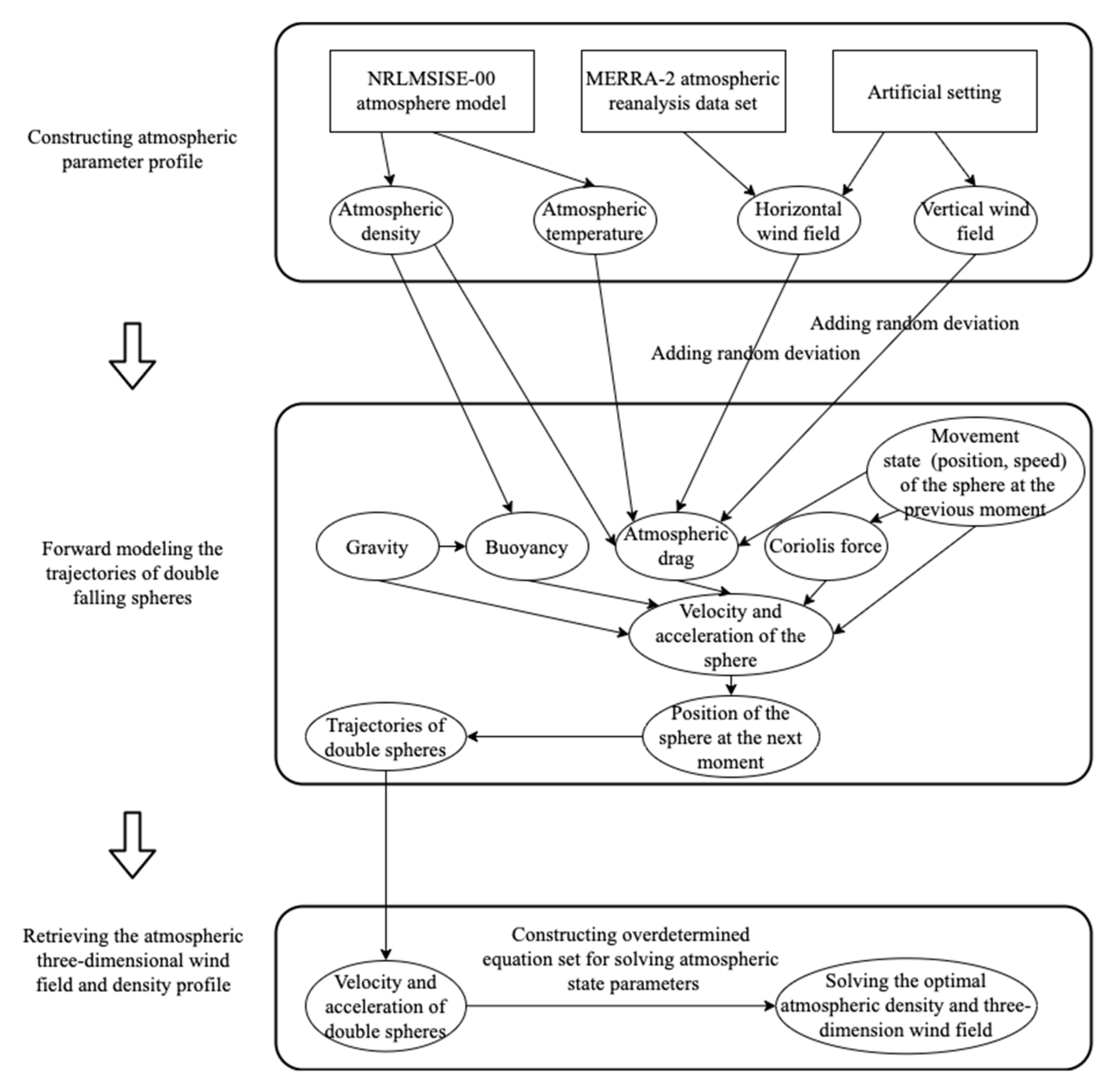
3.2.1. Constructing Atmospheric Parameter Profile

Figure 3 shows the neutral atmospheric density and temperature profile according to the NRLMSISE-00 atmosphere model.

The horizontal wind field from 20 to 60 km provided by the MERRA-2 data set was used as the simulated corresponding height horizontal wind field, while the horizontal wind field from 60 to 100 km and the vertical wind field were artificially set. Some researchers have pointed out that the vertical wind speed can reach several meters per second at heights of 30–50 km [31] and even reach approximately 25 m/s at heights of approximately 80 km [28]. Based on these conclusions, the simulated three-dimensional wind field (Figure 4) was used as the background three-dimensional wind field within a small temporal and spatial scale.

3.2.2. Forward-Modeling Trajectories of Double Falling Spheres

This paper simulates the trajectories of two falling spheres with different mass-to-area ratios in the simulated atmospheric environment mentioned above. The sphere with a smaller mass-to-area ratio was used as the datum sphere, while the other sphere with a larger mass-to-area ratio was used as the auxiliary sphere. The trajectories of the two falling spheres in the simulated atmosphere were calculated with a time step of 0.5 s; that is, the position, velocity and acceleration of the falling spheres were calculated every half second, and the movement of the falling spheres was regarded as uniform acceleration motion in each calculation step.

The masses of the falling spheres used in the simulation experiment were both 0.28 kg, and the radii of the datum and auxiliary sphere were 0.6 m and 0.5 m. Before simulating the descending processes of the two falling spheres separately, the highest positions of the two falling spheres and the horizontal motion speeds at the highest positions need to be given as the initial condition of the simulation. When calculating the trajectories of the two spheres, the random deviation should be added to the three-dimensional wind field at each height layer. The amplitude of the random deviations is 10% of the true value of the wind speed and satisfies the random distribution rather than the normal distribution. Figure 5 shows the trajectories of the double falling spheres in which the values of x, y and h are the components of the zonal, meridional, and vertical displacements of the falling spheres, respectively, relative to the observation station.

3.2.3. Retrieving 3D Wind Field and Density Profile

According to the trajectories of double falling spheres obtained through forward-modeling, the speed and acceleration of the two spheres at different heights are available. Additionally, the speed and acceleration of the auxiliary falling sphere need to be interpolated to the same heights as those of the datum falling sphere, i.e., the time step (0.5 s) of the inversions is that of the calculated heights of the datum falling sphere during the forward-modeling process. Then, the optimal atmospheric density and three-dimensional wind field can be calculated by Equation set (6). Finally, the retrieved atmospheric parameter profiles need to be smoothed.

4. Results

4.1. Inversion Results of the Atmospheric 3D Wind Field

Figure 6 compares the three-dimensional wind field profile calculated by the trajectories of the double falling spheres with the constructed three-dimensional simulated wind field profile. It should be noted that the simulated wind profiles in Figure 4 or Figure 6 are just individual cases. For the convenience of description, this paper carries out inversion and analysis of these individual cases. The retrieved horizontal wind field is highly consistent with the simulated horizontal wind field, especially at altitudes below 50 km, and both almost completely overlapped. There was a relatively larger deviation between the retrieved horizontal wind field and the simulated horizontal wind field at altitudes of approximately 80 km and 90 km. The retrieved vertical wind was also more accurate at altitudes below 50 km but cannot reflect the actual condition of the vertical wind field above 60 km.

In the results of the wind field inversion conducted in this paper, the deviation of the retrieved zonal wind (Figure 7a) was less than 2 m/s below 60 km; the deviation of the retrieved meridional wind field (Figure 7b) was less than 2 m/s below 50 km and was approximately 3 m/s at a height of approximately 55 km; and the deviation of the retrieved vertical wind (Figure 7c) was less than 2 m/s below 58 km. In general, the deviation of the vertical wind was greater than that of the horizontal wind field, and the deviation of the wind field at high altitude was greater than that at low altitude.

4.2. Inversion Results of Atmospheric Density Profile

Figure 8 shows the inversion results of the atmospheric density using the double-falling-sphere method, which were in agreement with the simulated atmospheric density results (within an order of magnitude). The deviation of the retrieved atmospheric density increases with decreasing altitude, but the deviation rate of density was generally not more than 20%, especially at altitudes below 60 km, where it was not more than 5%.

4.3. Comparison with the Inversion Results of the Single-Falling-Sphere Method

As a comparison, the horizontal wind field and atmospheric density profile are also retrieved by using trajectory data of a single falling sphere (datum falling sphere). The vertical wind speed was assumed to be zero during the inversion process. Figure 9 shows the deviation profile of the atmospheric parameters retrieved by the single-falling-sphere method.

In general, the deviations of the horizontal wind field retrieved by the double-falling-sphere method and single-falling-sphere method were roughly the same, and the single-falling-sphere method had even higher accuracy than the double-falling-sphere method at some altitude.

The atmospheric density retrieved by the double-falling-sphere method had obviously higher accuracy than that retrieved by the single-falling-sphere method. Additionally, the atmospheric density retrieved by the single-falling-sphere method showed obvious negative deviation below 60 km and an obvious positive deviation above 80 km in Figure 9c, while the density retrieved by the double-falling-sphere method did not show obvious positive or negative deviation under 60 km in Figure 8c. Moreover, the density deviation rate of the double-falling-sphere method basically oscillates around zero below 60 km, which is much smaller than that of the single-falling-sphere method. At low altitudes, the deviation rate of the atmospheric density retrieved by the double-falling-sphere method was less than 5%, while the maximum deviation rate of density retrieved by the single-falling-sphere method was more than 10%.

5. Discussion

5.1. Wind Field Deviation Formula

In the inversion results of the three-dimensional wind field and atmospheric density profile by the double-falling-sphere method, both the deviation of the wind field and the deviation rate of the atmospheric density show the same characteristics: a small oscillation amplitude at low altitude (30–60 km), and a large oscillation amplitude at high altitude (60–100 km). In fact, there is a certain relationship between the deviation of the three-dimensional wind field and the deviation rate of the atmospheric density.

Suppose that the retrieved atmospheric density at a certain altitude is $k_1$ times the real atmospheric density, i.e., $\rho =k_1{\rho }_0$, where $\rho$ is the retrieved atmospheric density and ${\rho }_0$ is the actual atmospheric density. The drag coefficient is related to density; therefore, the deviation of retrieved density can lead to the deviation of the drag coefficient, which results in $C_d=k_2{C}_{d0}$, where $C_d$ is the calculated drag coefficient in the inversion process and $C_{d0}$ is the actual drag coefficient during the falling process of the sphere.

The drag force of the falling sphere is expressed as

$$m|\stackrel{\rightharpoonup }{a_d}|=\frac{1}{2}{\rho }_{0}A{C}_{d0}{\left|\stackrel{\rightharpoonup }{v_{r0}}\right|}^2$$

(8)

$$m\stackrel{\rightharpoonup }{a_d}=-\frac{1}{2}{\rho }_{0}A{C}_{d0}\left|\stackrel{\rightharpoonup }{v_{r0}}\right|\stackrel{\rightharpoonup }{v_{r0}}=-\frac{1}{2}{\rho }_{0}A{C}_{d0}\left|\stackrel{\rightharpoonup }{v_{r0}}\right|\left(\stackrel{\rightharpoonup }{v}-\stackrel{\rightharpoonup }{w_0}\right),$$

(9)

where $\stackrel{\rightharpoonup }{v_{r0}}$ is the actual airspeed and $\stackrel{\rightharpoonup }{w_0}$ is the actual wind field.

In the case of density deviation and let $k=k_1{k}_2$, the drag force of the falling sphere can also be expressed as

$$m|\stackrel{\rightharpoonup }{a_d}|=\frac{1}{2}{k}_1{k}_2{\rho }_{0}A{C}_{d0}{\left|\stackrel{\rightharpoonup }{v_r}\right|}^2=\frac{1}{2}k{\rho }_{0}A{C}_{d0}{\left|\stackrel{\rightharpoonup }{v_r}\right|}^2$$

(10)

$$m\stackrel{\rightharpoonup }{a_d}=-\frac{1}{2}{k}_1{k}_2{\rho }_{0}A{C}_{d0}\left|\stackrel{\rightharpoonup }{v_r}\right|\stackrel{\rightharpoonup }{v_r}=-\frac{1}{2}k{\rho }_{0}A{C}_{d0}\left|\stackrel{\rightharpoonup }{v_r}\right|\left(\stackrel{\rightharpoonup }{v}-\stackrel{\rightharpoonup }{w}\right),$$

(11)

where $\stackrel{\rightharpoonup }{v_r}$ and $\stackrel{\rightharpoonup }{w}$ are the calculated airspeed and wind field in the inversion process, respectively.

Through (8) and (10), we can obtain the following Equation:

$$\left|\stackrel{\rightharpoonup }{v_r}\right|=\frac{\left|\stackrel{\rightharpoonup }{v_{r0}}\right|}{\sqrt{k}}$$

(12)

Therefore, Equation (11) can be expressed as

$$m\stackrel{\rightharpoonup }{a_d}=-\frac{1}{2}\sqrt{k}{\rho }_{0}A{C}_{d0}\left|\stackrel{\rightharpoonup }{v_{r0}}\right|\left(\stackrel{\rightharpoonup }{v}-\stackrel{\rightharpoonup }{w}\right).$$

(13)

Through Equations (9) and (13), the relationship between the retrieved 3D wind field and the real 3D wind field can be expressed as

$$\stackrel{\rightharpoonup }{w}=\frac{\stackrel{\rightharpoonup }{w_0}-\left(1-\sqrt{k}\right)\stackrel{\rightharpoonup }{v}}{\sqrt{k}}.$$

(14)

Additionally, the deviation between the retrieved wind field and the actual wind field is

$$\mathsf{∆}\stackrel{\rightharpoonup }{w}=\stackrel{\rightharpoonup }{w}-\stackrel{\rightharpoonup }{w_0}=-\frac{\left(1-\sqrt{k}\right)}{\sqrt{k}}\left(\stackrel{\rightharpoonup }{v}-\stackrel{\rightharpoonup }{w_0}\right)=-\frac{\left(1-\sqrt{k}\right)}{\sqrt{k}}\stackrel{\rightharpoonup }{v_{r0}}.$$

(15)

Therefore, the deviation $\mathsf{∆}\stackrel{\rightharpoonup }{w}$ is positively correlated with $k$ (the product of $k_1$ and $k_2$) and $\stackrel{\rightharpoonup }{v_{r0}}$ (the actual airspeed).

Figure 10 shows the variation curves of airspeed with altitude during the falling process. It presents the characteristics of higher airspeed at high altitudes and lower airspeed at low altitudes. Through simulation experiments, it is found that the deviation of the drag coefficient also increases with the increase in the atmospheric density deviation rate. Therefore, according to the formula in Equation (15), the wind field deviation should meet the characteristics that the deviation is smaller at lower heights but greater at higher heights.

The three-dimensional wind field retrieved by the double-falling-sphere method has higher accuracy at lower altitudes. Additionally, the deviation of the calculated wind field can be effectively reduced by decreasing the mass-to-area ratios of the falling spheres to reduce the airspeed of the spheres.

5.2. Error Sources

In this simulation experiment, the retrieved parameters have a larger deviation above 60 km. Three main causes of the deviation are summarized as below:

(1)

The difference in the area-to-mass ratios. Due to the difference, the two spheres in the experiments pass through different spatial positions and there must be a certain difference in the atmospheric density, temperature, and wind field which affect the two spheres (this is the reason for adding random perturbations to the wind field during the forward-modeling process). Therefore, there must be deviation in the optimal atmospheric density calculated by the two spheres’ trajectories. Moreover, the added random wind perturbations are more likely to cause a larger density deviation rate at high altitudes due to the thin atmosphere. According to Equation (15), the density deviation can further cause the wind field deviation.

(2)

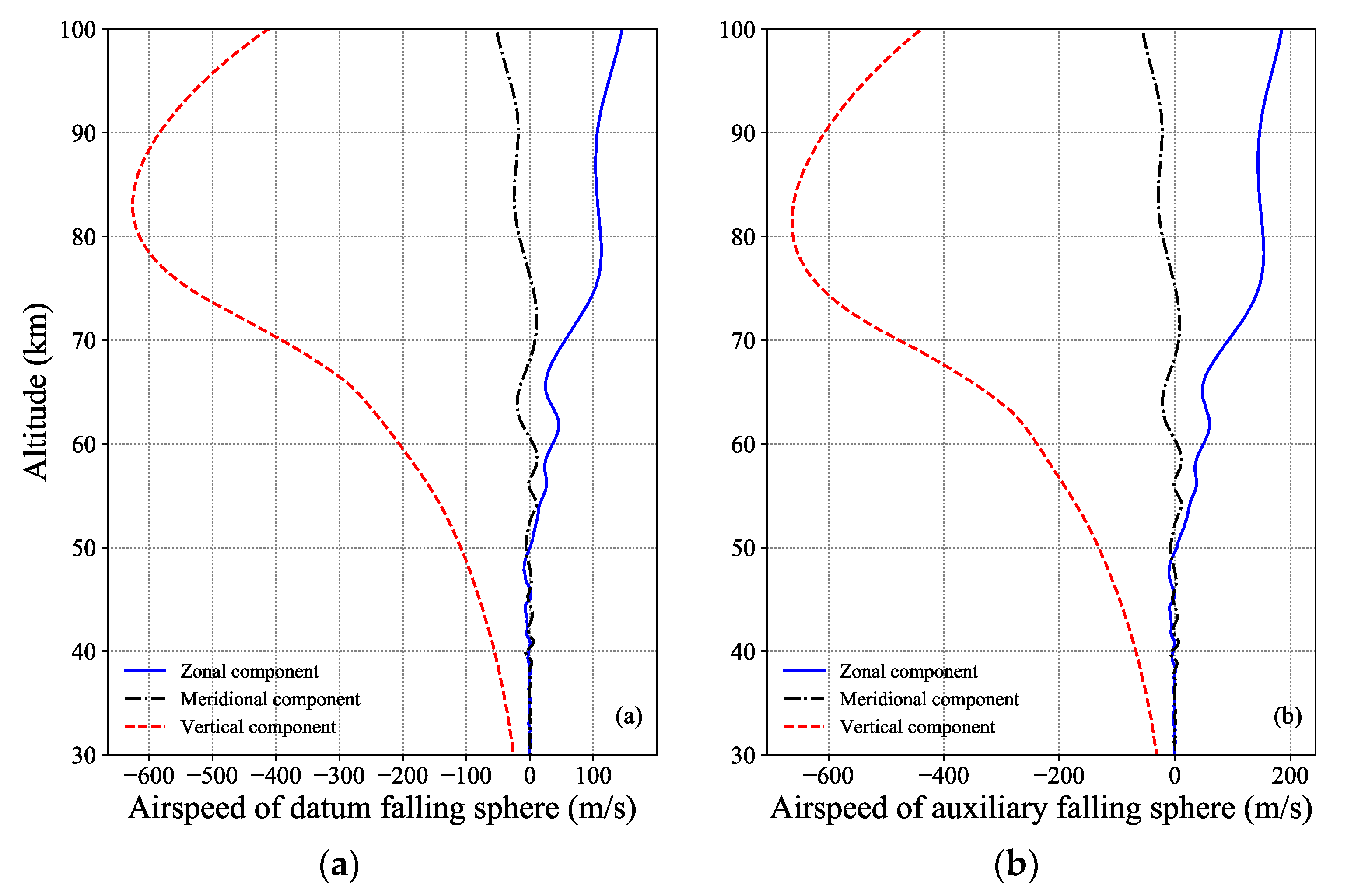
The airspeeds of the spheres are very large above 60 km. It is clear that the larger the airspeed is, the larger the deviation of the retrieved wind field will be according to Equation (15). Moreover, the trajectories data of the falling spheres is sampled at 0.5 s interval, so the height interval between two adjacent sampling points above 60 km are obviously larger than that at low altitude, which leads to the inaccuracy of temperature inversion and further lead to the deviation of the drag coefficient.

(3)

There is no clear physical formula for calculating the drag coefficient for now. The drag coefficient can only be achieved by experimental data or empirical formulas. Due to the difficulty of obtaining the true value of the drag coefficient, it is hard to access the impacts of the deviation of the drag coefficient to the inversion results.

6. Conclusions

In this paper, a simulation experiment is designed to verify the feasibility of retrieving the atmospheric density and three-dimensional wind field by the double-falling-sphere method. It is remarkable that in this simulation experiment, random deviation should be added to the wind field during the forward-modeling of the trajectories of the double spheres to simulate the difference between the average wind field and the actual wind field at different time and space positions. The results of the simulation experiment show that a credible vertical wind field and more accurate atmospheric density can be obtained by using the double-falling-sphere method at lower altitudes. The conclusions are as follows:

(1)

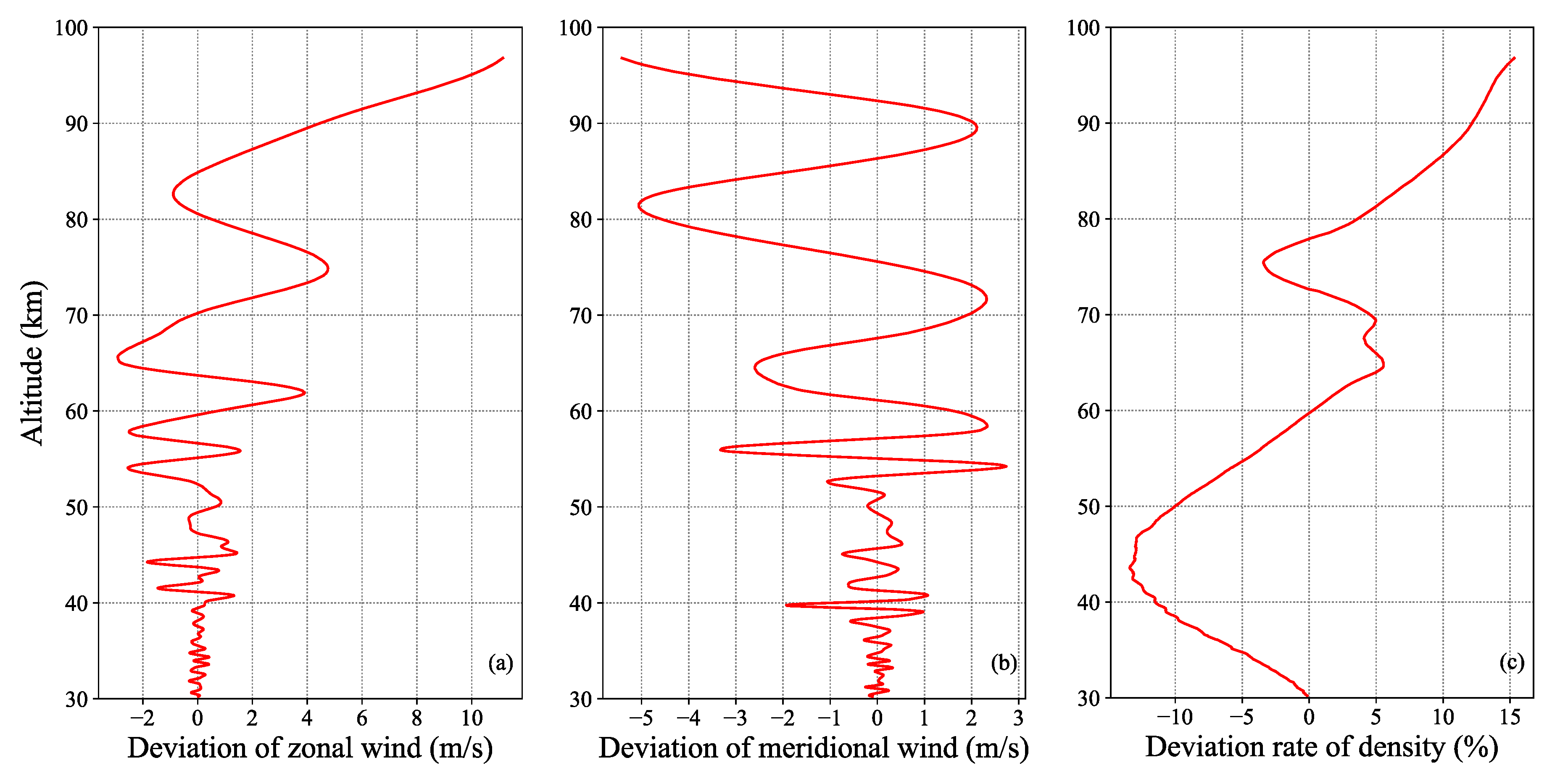
The retrieved atmospheric density is consistent with the simulated atmospheric density by an order of magnitude and has higher accuracy at low altitudes. It shows the characteristics of a larger deviation rate at higher altitudes and a smaller deviation rate at lower altitudes. The deviation rate of the retrieved density is generally not more than 20% and not more than 5% below 60 km.

(2)

Compared with the single-falling-sphere method, the atmospheric density calculated from the double falling spheres has higher accuracy at lower altitudes. The results show that the atmospheric density retrieved by the single-falling-sphere method has obvious positive deviation or negative deviation, while the deviation rate of density retrieved by the double-falling-sphere method oscillates around zero below 60 km.

(3)

The retrieved horizontal wind field is in high agreement with the simulated wind field, and the vertical wind field below 60 km is more accurate than that above 60 km. In the results of the simulation experiment in this paper, the deviation of each component of the three-dimensional wind field is generally less than 3 m/s below 60 km. In general, the retrieved three-dimensional wind field has high accuracy at altitudes below 60 km.

(4)

The deviation of the retrieved three-dimensional wind field is related to the deviation rate of the retrieved density and the actual airspeed. There are smaller density deviation rates and airspeeds at lower altitudes and larger density deviation rates and airspeeds at higher altitudes, so the wind field should also show the characteristics of larger deviations at higher altitudes and smaller deviations at lower altitudes according to the derived wind field deviation formula. This conclusion is consistent with the experimental results.

(5)

To reduce the deviation of the retrieved wind field, falling spheres with small mass-to-area ratios should be used to retrieve the three-dimensional wind field. Falling spheres with small mass-to-area ratios are more easily affected by wind, so the airspeed is smaller. According to the wind field deviation formula, the smaller the airspeed is, the smaller the deviation of the retrieved wind field will be.

References

1. Smith, A.K. Interactions between the lower, middle and upper atmosphere. Space Sci. Rev. 2012, 168, 1–21. [Google Scholar] [CrossRef]
2. Andrews, D.G.; Holton, J.R.; Leovy, C.B. Middle Atmosphere Dynamics; Academic Press: San Diego, CA, USA, 1987; pp. 1–2. [Google Scholar]
3. Chen, Z.Y.; Chen, H.B.; Xu, J.Y.; Huang, K.M.; Xue, X.H.; Hu, D.Z.; Chen, W.; Yang, G.T.; Tian, W.S.; Hu, Y.Y.; et al. Advances in the researches of the middle and upper atmosphere in China. Chin. J. Space Sci. 2020, 40, 856–874. [Google Scholar]
4. He, Y.; Sheng, Z.; He, M.Y. Spectral analysis of gravity waves from near space high-resolution balloon data in northwest. Atmosphere 2020, 11, 133. [Google Scholar] [CrossRef] [Green Version]
5. He, Y.; Sheng, Z.; He, M.Y. The interaction between the turbulence and gravity wave observed in the middle stratosphere based on the round-trip intelligent sounding system. Geophys. Res. Lett. 2020, 47, e2020GL088837. [Google Scholar] [CrossRef]
6. Sheng, Z.; Zhou, L.S.; He, Y. Retrieval and Analysis of the Strongest Mixed Layer in the Troposphere. Atmosphere 2020, 11, 264. [Google Scholar] [CrossRef] [Green Version]
7. Hagen, J.; Murk, A.; Rüfenacht, R.; Khaykin, S.; Hauchecorne, A.; Kämpfer, N. WIRA-C: A compact 142-GHz-radiometer for continuous middle-atmospheric wind measurements. Atmos. Meas. Tech. 2018, 11, 5007–5024. [Google Scholar] [CrossRef]
8. Wang, H.M.; Yan, H.H.; Fu, L.P.; Zhang, X.X.; Zong, W.G. Wind retrieval of Fabry-Perot interferometer in the middle and upper atmosphere using wavelength depth method based on satellite-based simulation and ground-based measurement. Eur. J. Remote Sens. 2020, 53, 145–155. [Google Scholar] [CrossRef]
9. Wang, H.M.; Wang, C.; Wang, Y.M.; Zhang, X.X.; Huang, C.; Liang, S.L. Retrieval of middle and upper atmospheric wind based on non-full circular fringe recorded by Fabry-Perot Interferometer. Sci. China-Earth Sci. 2017, 60, 1732–1738. [Google Scholar] [CrossRef]
10. Baron, P.; Murtagh, D.; Eriksson, P.; Mendrok, J.; Ochiai, S.; Pérot, K.; Sagawa, H.; Suzuki, M. Simulation study for the Stratospheric Inferred Winds (SIW) sub-millimeter limb sounder. Atmos. Meas. Tech. 2018, 11, 4545–4566. [Google Scholar] [CrossRef] [Green Version]
11. Grawe, M.A.; Chu, K.T.; Makela, J.J. Measurement of atmospheric neutral wind and temperature from Fabry–Perot interferometer data using piloted deconvolution. Appl. Opt. 2019, 58, 3685–3695. [Google Scholar] [CrossRef]
12. Langille, J.A.; Ward, W.E.; Nakamura, T. First mesospheric wind images using the Michelson interferometer for airglow dynamics imaging. Appl. Opt. 2016, 55, 10105–10118. [Google Scholar] [CrossRef] [PubMed]
13. Liu, J.L.; Wei, D.K.; Zhu, Y.J.; Kaufmann, M.; Olschewski, F.; Mantel, K.; Xu, J.Y.; Riese, M. Effective wind and temperature retrieval from Doppler asymmetric spatial heterodyne spectrometer interferograms. Appl. Opt. 2018, 57, 8829–8835. [Google Scholar] [CrossRef] [PubMed]
14. Jacobi, C.; Fröhlich, K.; Viehweg, C.; Stober, G.; Kürschner, D. Midlatitude mesosphere/lower thermosphere meridional winds and temperatures measured with meteor radar. Adv. Space Res. 2007, 39, 1278–1283. [Google Scholar] [CrossRef]
15. Dou, X.K.; Han, Y.L.; Sun, D.S.; Xia, H.Y.; Shu, Z.F.; Zhao, R.C.; Shangguan, M.J.; Guo, J. Mobile Rayleigh Doppler lidar for wind and temperature measurements in the stratosphere and lower mesosphere. Opt. Express 2014, 22, A1203–A1221. [Google Scholar] [CrossRef] [PubMed]
16. Shu, Z.F.; Tang, L.; Jiang, S.; Li, Z.M.; Zhao, R.C.; Zheng, J. Improving the efficiency of doppler lidar receiver for upper atmospheric wind field measurement. Optik 2017, 149, 169–173. [Google Scholar] [CrossRef]
17. Sharma, A.K.; Gaikwad, H.P.; Ratnam, M.V.; Gurav, O.B.; Ramanjaneyulu, L.; Chavan, G.A.; Sathishkumar, S. Diurnal, monthly and seasonal variation of mean winds in the MLT region observed over Kolhapur using MF radar. J. Atmos. Sol.-Terr. Phys. 2018, 169, 91–100. [Google Scholar] [CrossRef]
18. Schmidlin, F.J.; Lee, H.S.; Michel, W. The inflatable sphere: A technique for the accurate measurement of middle atmosphere temperatures. J. Geophys. Res.-Atmos. 1991, 96, 22673–22682. [Google Scholar] [CrossRef]
19. Fan, Z.Q. Analysis and Research of Atmospheric Sounding Data in Near Space. Ph.D. Thesis, National University of Defense Technology, Changsha, China, March 2018. (In Chinese). [Google Scholar]
20. Bartman, F.L.; Chaney, L.W.; Jones, L.M.; Liu, V.C. Upper-air density and temperature by the falling-sphere method. J. Appl. Phys. 1956, 27, 706–712. [Google Scholar] [CrossRef] [Green Version]
21. Otterman, J.; Sattinger, I.J.; Smith, D.F. Analysis of a falling-sphere experiment for measurement of upper-atmosphere density and wind velocity. J. Geophys. Res. 1961, 66, 819–822. [Google Scholar] [CrossRef]
22. Faucher, G.A.; Morrissey, J.F.; Stark, C.N. Falling sphere density measurements. J. Geophys. Res. 1967, 72, 299–305. [Google Scholar] [CrossRef]
23. Yuan, Y.; Ivchenko, N.; Tibert, G.; Stanev, M.; Hedin, J.; Gumbel, J. Atmosphere density measurements using GPS data from rigid falling spheres. Atmos. Meas. Tech. Discuss. 2017. [Google Scholar] [CrossRef] [Green Version]
24. Ge, W.; Sheng, Z.; Zhang, Y.Y.; Fan, Z.Q.; Cao, Y.; Shi, W.L. The study of in situ wind and gravity wave determination by the first passive falling-sphere experiment in China’s northwest region. J. Atmos. Sol.-Terr. Phys. 2019, 182, 130–137. [Google Scholar] [CrossRef]
25. Peterson, J.W.; Hansen, W.H.; McWatters, K.D.; Bonfanti, G. Falling sphere measurements over Kwajalein. J. Geophys. Res. 1965, 70, 4477–4489. [Google Scholar] [CrossRef]
26. Zhang, Y.Y. Analysis and Application of Wind and Temperature Detection Data in Middle and Upper Atmosphere. Master’s Thesis, National University of Defense Technology, Changsha, China, October 2017. (In Chinese). [Google Scholar]
27. Brekke, A. The atmosphere of the Earth. In Physics of the Upper Polar Atmosphere, 2nd ed.; Springer: Berlin/Heidelberg, Germany, 2013; pp. 51–115. [Google Scholar]
28. Jones, L.M.; Peterson, J.W. Falling sphere measurements, 30 to 120 km. In Meteorological Investigations of the Upper Atmosphere; American Meteorological Society: Boston, MA, USA, 1968; pp. 176–189. [Google Scholar]
29. Cheng, X.X.; Hu, X.; Xiao, C.Y.; Wang, X.J. Correction method of the low earth orbital neutral density prediction based on the satellites data and NRLMSISE-00 model. Chin. J. Geophys. 2013, 56, 3246–3254. (In Chinese) [Google Scholar]
30. Henderson, C.B. Drag coefficients of spheres in continuum and rarefied flows. AIAA J. 1976, 14, 707–708. [Google Scholar] [CrossRef]
31. Hildreth, W.W. Special problems of measurement below 100 km. In Meteorological Investigations of the Upper Atmosphere; American Meteorological Society: Boston, MA, USA, 1968; pp. 222–224. [Google Scholar]
32. Shi, Y.H. An optimization algorithm based on brainstorming process. Int. J. Swarm Intell. Res. 2011, 2, 35–62. [Google Scholar] [CrossRef]
33. Bao, G.; Li, J.; Huang, R.T.; Shen, K.X. An improved brainstorm optimization algorithm based on the strategy of random perturbation and vertical variation. In Proceedings of the 38th Chinese Control Conference, Guangzhou, China, 27–30 July 2019; pp. 2046–2051. [Google Scholar]
34. Zhang, N. Intelligent Optimization Algorithms for Solving Nonlinear Equations. Master’s Thesis, Jilin University, Changchun, China, April 2013. (In Chinese). [Google Scholar]
Figure 1. Drag coefficient summarized by Henderson. (Ma is Mach number, Re is Reynolds number, and Cd is drag coefficient).
Atmosphere 11 01312 g001
Figure 2. Flow chart of the simulation experiment.
Atmosphere 11 01312 g002
Figure 3. (a) Atmospheric density and (b) temperature profile provided by the NRLMSISE-00 atmosphere model.
Atmosphere 11 01312 g003
Figure 4. The simulated three-dimensional wind field. (a) Zonal wind; (b) meridional wind; (c) vertical wind.
Atmosphere 11 01312 g004
Figure 5. Forward-modeled trajectories of double falling spheres. (a) Zonal displacement; (b) meridional displacement; (c) vertical displacement.
Atmosphere 11 01312 g005
Figure 6. Comparison of smoothed 3D wind field inversion results with the simulated wind field. (a) Zonal wind; (b) meridional wind; (c) vertical wind.
Atmosphere 11 01312 g006
Figure 7. Deviation of the retrieved three-dimensional wind field. (a) Deviation of the zonal wind; (b) deviation of the meridional wind; (c) deviation of the vertical wind.
Atmosphere 11 01312 g007
Figure 8. Inversion result of the atmospheric density profile. (a) Comparison of the retrieved atmospheric density profile with the simulated atmospheric density profile; (b) deviation of the density (the absolute value of the difference between the retrieved density and the simulated density); (c) Deviation rate of the density (the ratio between the deviation of the density and the simulated density).
Atmosphere 11 01312 g008
Figure 9. Inversion deviation of the single-falling-sphere method. (a) Deviation of the zonal wind; (b) deviation of the meridional wind; (c) deviation rate of the density.
Atmosphere 11 01312 g009
Figure 10. Airspeed of double spheres during the falling process. (a) Airspeed of the datum falling sphere; (b) airspeed of the auxiliary falling sphere.
Atmosphere 11 01312 g010
Publisher’s Note: MDPI stays neutral with regard to jurisdictional claims in published maps and institutional affiliations.