1. Introduction
The Antarctic Peninsula (AP), including the South Shetland Islands, is a complex mountainous glacier system, with more than 1100 individual glaciers descending from high elevations and draining to both sides of the peninsula, either into ice shelves, grounding or floating as marine glaciers [
1]. Near two-thirds of the Peninsula (the Graham Land) extends northward for about 1300 km with several peaks exceeding the 2000 m [
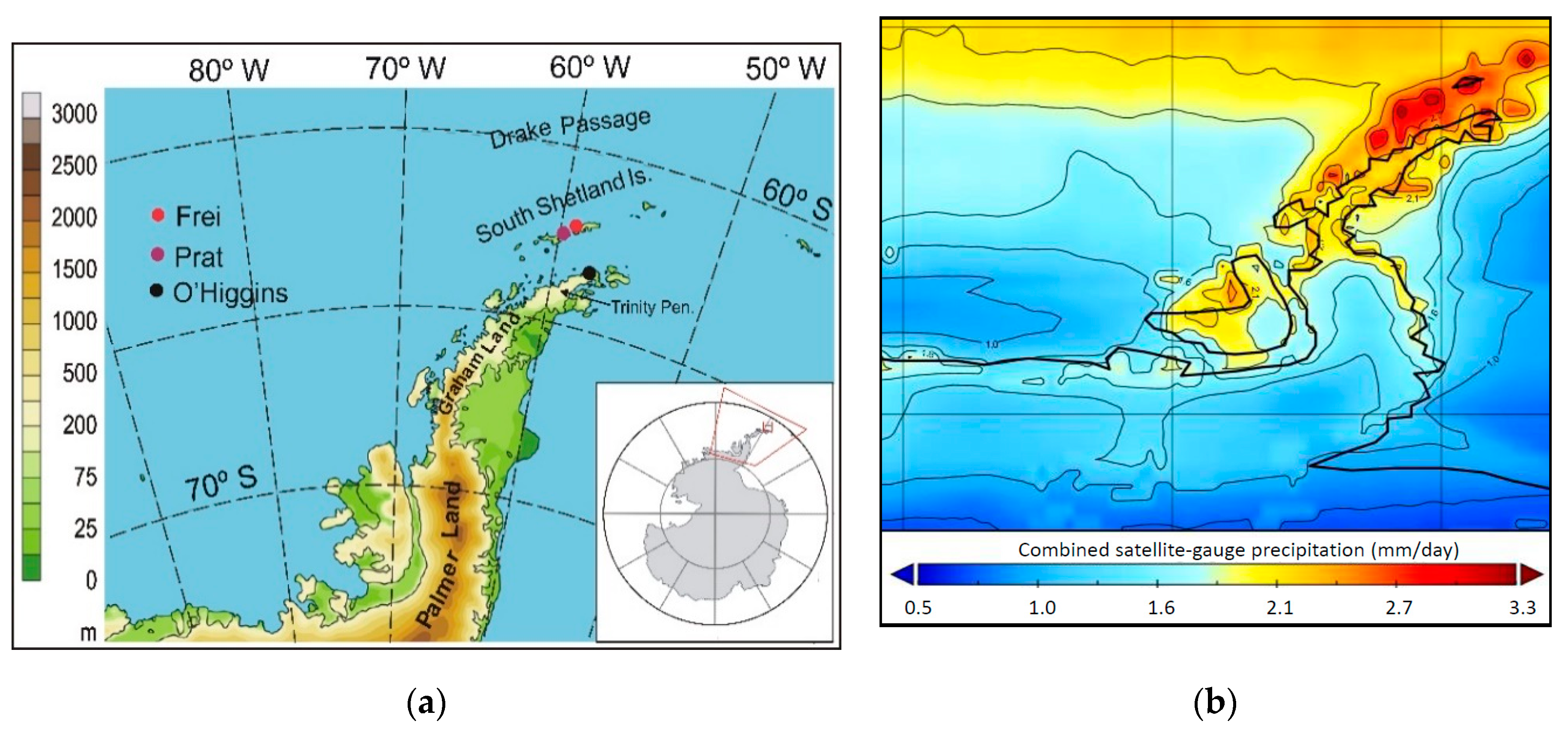
1], separating the southernmost Pacific and Atlantic oceans and leaving to the north the Drake Passage (
Figure 1a). AP extends in an almost north-south direction rising in opposition to the prevailing westerly airflow and as a source for mountain waves formation [
2]. It increases the windward precipitation on the western side and generates the föehn effect in the lee side, decreasing (increasing) the precipitation (near-surface air temperature) [
3,
4] in the Weddell-side of the AP. The climatological sea-level pressure resolves two near-permanent cyclonic circulations centered in the Southeastern Pacific Ocean and the Southern Atlantic Ocean (about 20° W, north of Queen Muad Land). These centers form part of the climatological zonal wave 3-patterns that surround the Antarctic continent as a result of the frequent activity of synoptic and subsynoptic weather systems in the southern oceans [
5] and the effect of the Antarctic topography [
6]. The cyclonic circulation at both sides of the peninsula yields to prevailing north/northwesterly winds advecting relatively warmer and moister air in its western side defining a sub-polar climate, while the almost permanent southerly winds support cold air advection from the continent in its eastern side defining a polar continental climate. This climatic difference is also manifested by other parameters like cloudiness, relative humidity, and precipitation/accumulation, which are higher over the western side [
7].
The dominant type of precipitation in the AP is snow mainly southern of 70° S, where air temperature usually is below 0 °C year-round. However, also, liquid precipitation can mainly occur during the summer, in the northern half of the Peninsula, even on a few occasions during the winter [
8]. Most of the precipitation is constrained to the coastal regions, and it is associated with a synoptic-scale weather system [
8] moving southeastward and crossing the AP and/or dissipating (frontolysis) in the southern oceans. Additionally, the topographic characteristic of the AP intensifies the precipitation in its western side by lifting the moving air mass, while the descending-adiabatic motion (Foehn winds) of the air mass inhibits precipitation over the eastern side [
4]. Therefore, as a result of the atmospheric circulation and the topography, the annual net accumulation distribution in the AP (
Figure 1b) shows a larger annual accumulation in its western side than its eastern side [
7,
9]. The Pacific coast of the southwestern AP and Ellsworth Land is the largest accumulation region of Antarctica [
7].
Figure 1b shows the average precipitation for the 1991–2010 period, constructed using the combined monthly satellite-gauge precipitation (AIRS, SSMI GPCPMON v3.0) data obtained from Giovanni webpage [
10], with a spatial resolution of 0.5° × 0.5° [
11]. Precipitation amount and type of precipitation changes in the AP is important for the local and regional surface mass balance. Type of precipitation changes can allow studying the atmospheric dynamics in the region, so that, liquid precipitation prevails with poleward warmer and moister transport, while solid precipitation prevails within cold air masses moving northward. Precipitation data are scarce in Antarctica, and the fact that this information is available in the northern tip of the AP allows to analyze its historical behavior under the framework of the global climate change and the impact on the AP region. In this article, the total annual and seasonal precipitation accumulation and precipitation days (defined as all day that registered at least 0.1 mm accumulated in 24 h), as well as precipitation types (rain and snow) recorded at the Antarctic Chilean Frei station, are analyzed. For this, linear trends and exponential curves were calculated for the 1970–2019 period to describe the long-term and the decadal-like changes. In addition, we explored whether or not changes in rainfall and snowfall events have occurred in the northern tip of the AP, as observed at this station located in King George Island. The next section describes the data and methodology used to analyze the precipitation behavior and changes, followed by the section where we discuss the findings and their implications finalizing with the conclusion section.
2. Materials and Methods
The three historical climate data from the weather stations Frei (62.2° S, 58.9° W, 10 m asl), Prat (62.5° S, 59.6° W, 5 m asl), and O’Higgins (63.3° S, 57.9° W 10 m asl) located in the AP (
Figure 1a) were downloaded from the Dirección Meteorológica de Chile (DMC) from the institutional webpage (
www.meteochile.gob.cl). Daily mean air temperature, precipitation accumulation, and type of precipitation were obtained from Frei station, where trained personnel (meteorological observers) operate year-round, while monthly precipitation data were available from Prat and O’Higgins stations. Frei and O’Higgins have been uninterruptedly in operation since 1969 and 1963, respectively, while Prat station has an interruption from 2004 to 2009. Monthly averages were calculated using the corresponding total precipitation from the three stations, and seasonal and annual accumulation averages were computed to obtain a more regional behavior from 1970 to 2019. The daily mean air temperature was constructed by averaging the minimum and maximum air temperature.
The daily (and monthly) precipitation corresponds to the sum of the rainfall and the snowfall water equivalent. Direct observations carried out by personnel at the Antarctic weather stations are scarce in the southern polar region, but also the accuracy and reliability of instrumental-based precipitation measurements in windy regions are usually affected by blowing/drifting snow [
12]. Wind-induced snow transport can produce snow deposition and removal leading to significant errors in the Surface Mass Balance (SMB) on a local and regional scale [
13]. Antarctic precipitation is the main positive term in the SMB [
14], and errors induced by the snow-drifting can overestimate the SMB in some places and underestimate in areas of snow-drifting erosion [
12]. In these three stations, atmospheric measurements are carried by personnel year-round, at Prat and O’Higgins they received a three-week training to carry out weather observations, and at Frei they are performed by meteorological technicians from DMC. Frei station reports every 3 h in the standard WMO (World Meteorological Organization) SYNOP format, the precipitation amount and the precipitation type falling at the time of the observation. These types include drizzle (DZ), rain (RA), rain-shower (RASH), snow (SN), snow-shower (SNSH), and mix of rain and snow (SNRA and SNRASH) and its intensities. This information is codified following the format FM12-VII/13-VII and is sent to the World Meteorological Centers through the Global Telecommunication System (GTS) of the WMO.
The data were obtained from DMC to construct a monthly number of events with the type of precipitation that was observed at Frei station. The events were categorized as drizzle, rain, and snow events (RASN and RASNSH were counted as snow). Snow precipitation falling within the station weather is measured every 6 h using a ruler where 1 cm of snow is equivalent to 1 mm of water. If the snow depth is less than 0.5 cm is defined as trace and codified as 0.0, while if the snow depth is between 0.6 and 0.9 mm, it is approximated to 1 cm (1 mm). No correction or adjustment due to wind speed and mixed phase is made to the original data. It was considered that wind-induced snow removal and accumulation can, on average, cancel each other, and there is no information about a characteristic of the snow for further analysis. Quality control was performed to eliminate all inconsistencies between daily precipitation measurements and the type of precipitation reported. Even though the observations were carried out by trained personal, at first glance some errors were found by crossing the precipitation days with the type of precipitation registered on those days. All days that reported precipitation type events, but they were not simultaneously accompanied by the amount of precipitation. This reduced the precipitation days amounts in about 23%, but the remnant data allow the comparing analysis between precipitation amount and precipitation days/events. In addition, all days that were reported as drizzle occurrence, but the days when the amount of precipitation was larger than 0.9 mm were considered either as a rainy day (if the mean air temperature was above 0.5 °C) or snowy day (if the air temperature was below 0.5 °C). This was determined by taking the average of the mean air temperature for the days with liquid and solid precipitation registered at Frei station.
Annual and seasonal averages and standard deviations were calculated for each station, along with the corresponding histograms to analyze the annual and seasonal behavior of precipitation accumulation and type events. In this study, Summer includes the December month of the previous year, for instance, summer 2010 covers December 2009, January, and February 2010. The other seasons are, as usual, autumn (March, April, and May), winter (June, July, and August), and spring (September, October, and November). In addition, additional statistic parameters were performed to obtain the coefficient of skewness (
Cs), kurtosis (
Ck), varied (
Cv), and the Durbin–Watson (DW) test for autocorrelation of each time series. In summary, the mathematical expressions are:
where
µ is the average of the series of n observations,
Md is the median,
s the standard deviation,
se is the standard error of the regression, and
are the residuals.
Additionally, the Shapiro–Wilk (SW) test was used to check normal distribution. The SW tests the null hypothesis that the sample of n observations came from normally distributed population, which is given by the expression:
where the data is previously rearranged in ascending order so that
,
is the
ith order statistic (it is the
ith-smallest number in the sample, and it is different from
xi). The coefficient
is given by
with
C defined as the vector norm.
The autocorrelation was also analyzed by estimating the effective number of the lag-1 autocorrelation coefficient (
) of
e(
t), following the method described by Santer et al. [
15]. For a regression line
(
t = 1,…,
nt), with trend
b and regression residuals,
e(
t), given by
, the standard error of
b is defined as
An effective sample
ne based on
is
With variance of the residuals about the regression line given by
To evaluate whether a trend is significantly different from zero, it is used the ratio between the estimated trend,
b, and the standard error,
se.
Assuming that tb is distributed as Student’s t-test, then it is compared with a critical t value (of significant level and nt−2 degree of freedom) to evaluate the null hypothesis b = 0. If e(t) is autocorrelated, then the null hypothesis is rejected.
Moreover, the nonparametric test Kendall’s tau rank correlation (τ) and Sen’s slope were performed to ensure the significance of the true trend of the time series. This is given by
where
is the binomial coefficient for the number of ways to choose two items from n items.
C is number of concordant pairs and
D is number of discordant pairs.
The Sen’s slope is defined as
with confidence interval calculated as lower =
x(N-k)/2 and upper =
x(N+k)/(2+1), where N =
and
k =
se ×
zcrit.
To assess the long-term variability (near decadal-like changes) of the time series, the interannual variability was filtered out using the exponential smoothing [
16] given by
where
yt is the average of the first 5–7 years of the series,
zt corresponds to the final value of the first smoothing,
c is the degree of smoothing (between 0 and 1), which was set to 0.25 to filter out the interannual variability while preserving the decadal behavior. Annual and seasonal trends were computed, including their statistically significant levels performing the linear regression analysis using the least squares method to fit a line through a set of observations, after filtering out the interannual variability.
3. Results
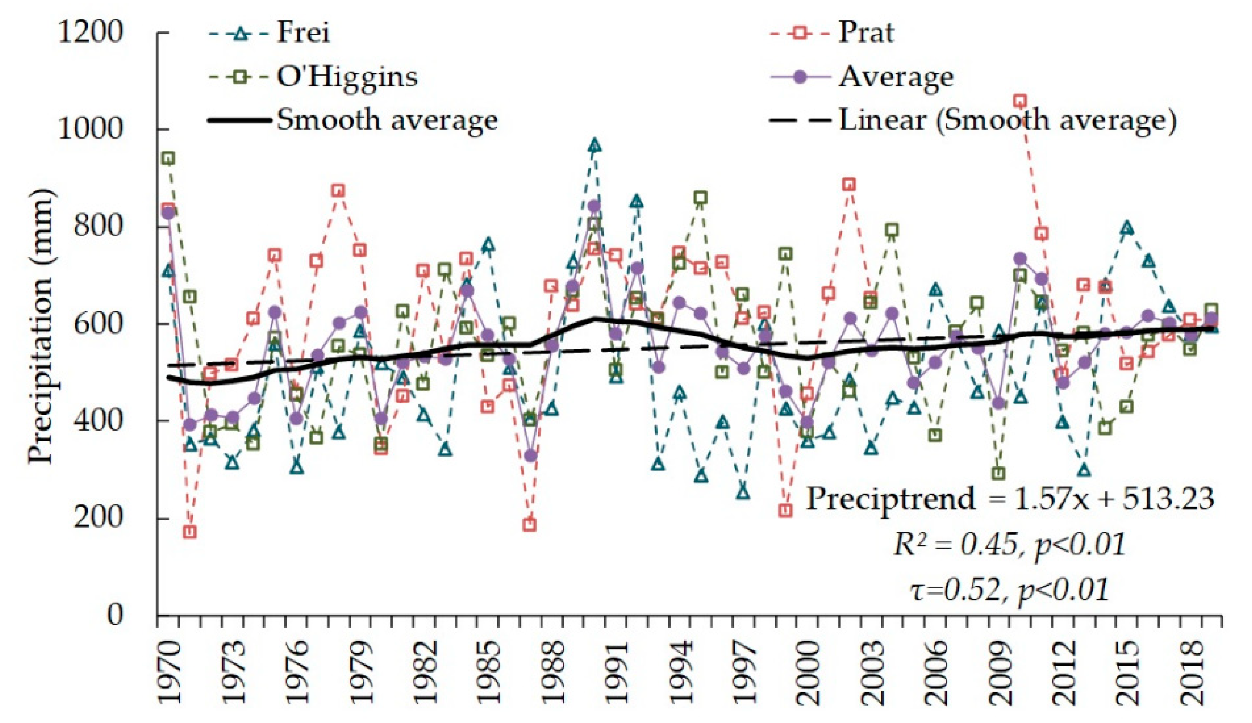
Precipitation in the AP and surrounding islands are highly variable.
Figure 2 depicts the annual precipitation accumulation by Frei, Prat, and O’Higgins stations revealing the temporal and spatial variability, the correlations among them are low and nonstatistically significant (
n.s.). All stations revealed positive linear trends that, on average, is around 16 ± 5 mm (10 year)
−1 (
p < 0.05) (hereafter the number following the ± sign corresponds to the 95% confidence intervals of the regression line). The areal average from the three stations can give us a closer near-real behavior of the precipitation in the northern tip of the AP. The exponential filter shows the decadal-like changes superimposed on the linear trends with increasing and decreasing precipitation periods throughout the 1970–2019 period. Thus, the exponential filter applied to the areal average reveals two positive trends: 1970–1991 and 2000–2019 with a statistically significant increase of 60 ± 7 mm (10 year)
−1 (
p < 0.05) and 31 ± 4 mm (10 year)
−1 p < 0.05), and a negative trend between 1991 and 1999 with decreasing precipitation of −95 ± 9 mm (10 year)
−1 (
p < 0.05).
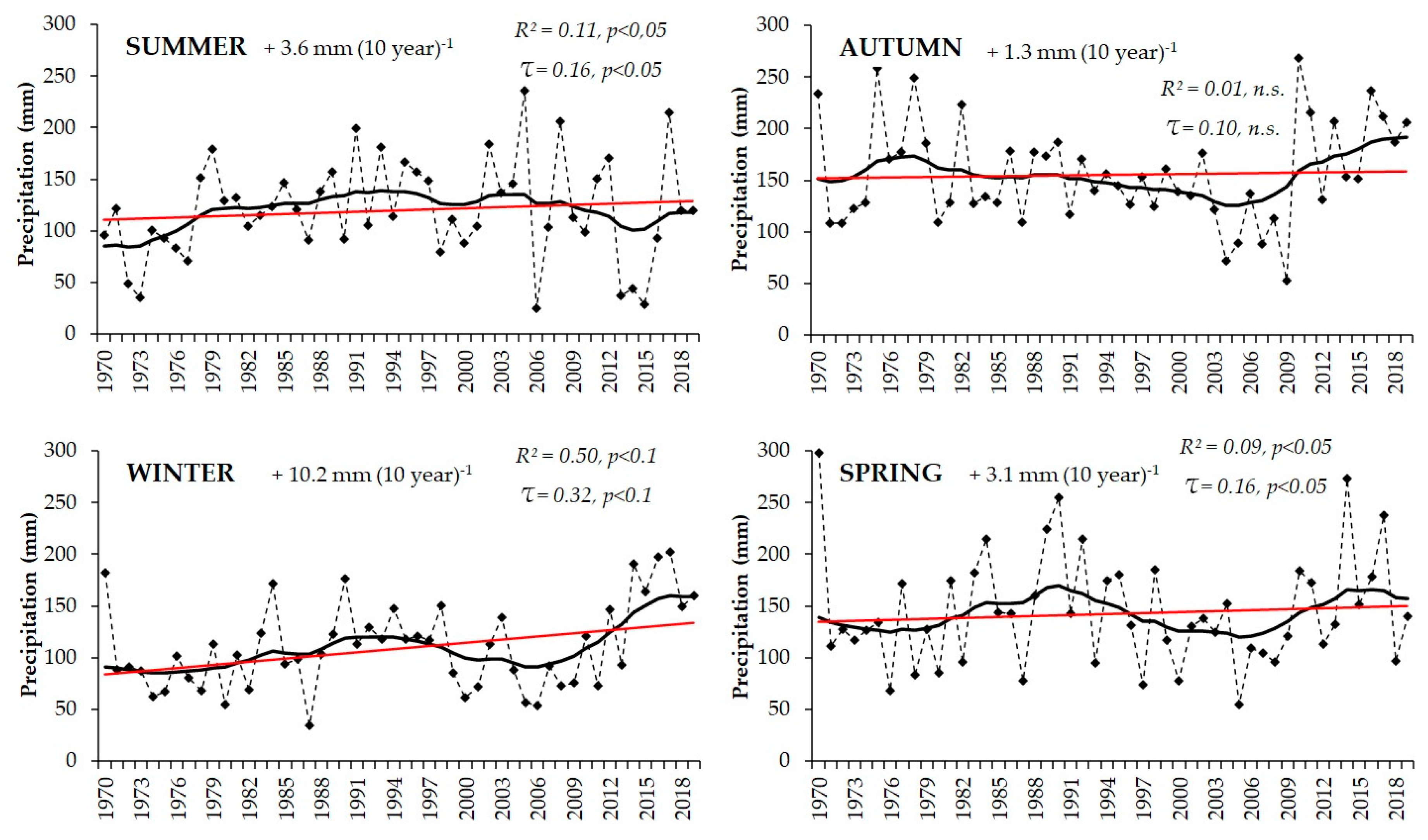
The seasonal areal behavior of the precipitation is given in
Figure 3. All seasons revealed positive statistically significant (
p < 0.05) trends over the 1970–2019 period, except in autumn, being winter the largest trend with around 10 ± 3 mm (10 year)
−1. However, the decadal-like analysis given by the exponential filter reveals periods of decreasing and increasing precipitation. The most remarkable statistically significant increases are from 1970 to 1992 during summer (+26 ± 4 mm (10 year)
−1,
p < 0.05), winter (+16 ± 3 mm (10 year)
−1,
p < 0.05), and spring (+20 ± 5 mm (10 year)
−1,
p < 0.05) and from the mid-2000s to 2019 during autumn (+39 ± 8 mm (10 year)
−1,
p < 0.05), winter (+41 ± 8 mm (10 year)
−1,
p < 0.05), and spring (+27 ± 6 mm (10 year)
−1,
p < 0.05). However, a significant decrease took place from 1992 to mid-2000s during winter (−24 ± 3 mm (10 year)
−1,
p < 0.05) and spring (−31 ± 6 mm (10 year)
−1,
p < 0.05) and also during autumn but from ~1976 to ~2006 (−14 ± 1 mm (10 year)
−1,
p < 0.05).
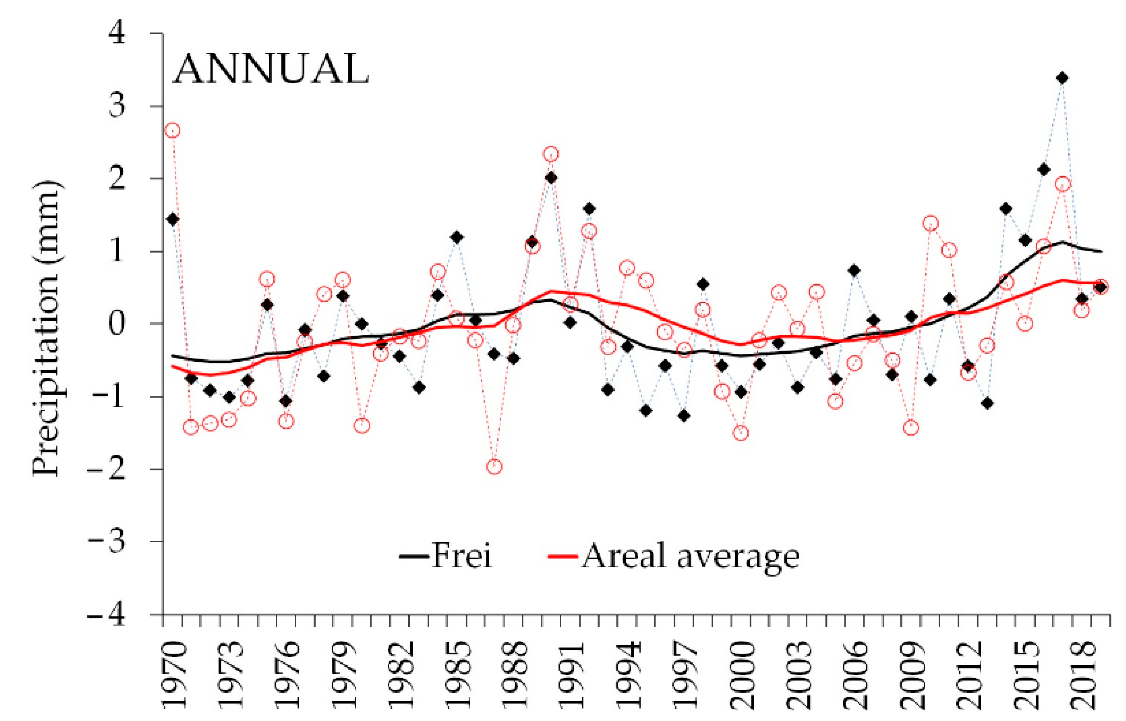
Figure 4 shows the standardized annual anomalies of the annual precipitation at Frei station and the areal average of Frei, Prat, and O’Higgins. The standardized anomalies were calculated by taking the difference between annual accumulation and the average over the 1970–2019 period and dividing by the standard deviation. The resulting curves reveal similar interannual and decadal behaviors (correlations of 0.65 and 0.84, both statistically significant at
p < 0.05), although some individual years can differ between both series. In addition, a comparison between the seasonal total precipitation at Frei and the areal-average shows similar behaviors. This overall agreement allows us to use the observational 3-hourly reports of the significant weather registered by trained personnel at Frei station and to count precipitation events and categorize them according to their type and derive the overall behavior in the northern tip of the AP.
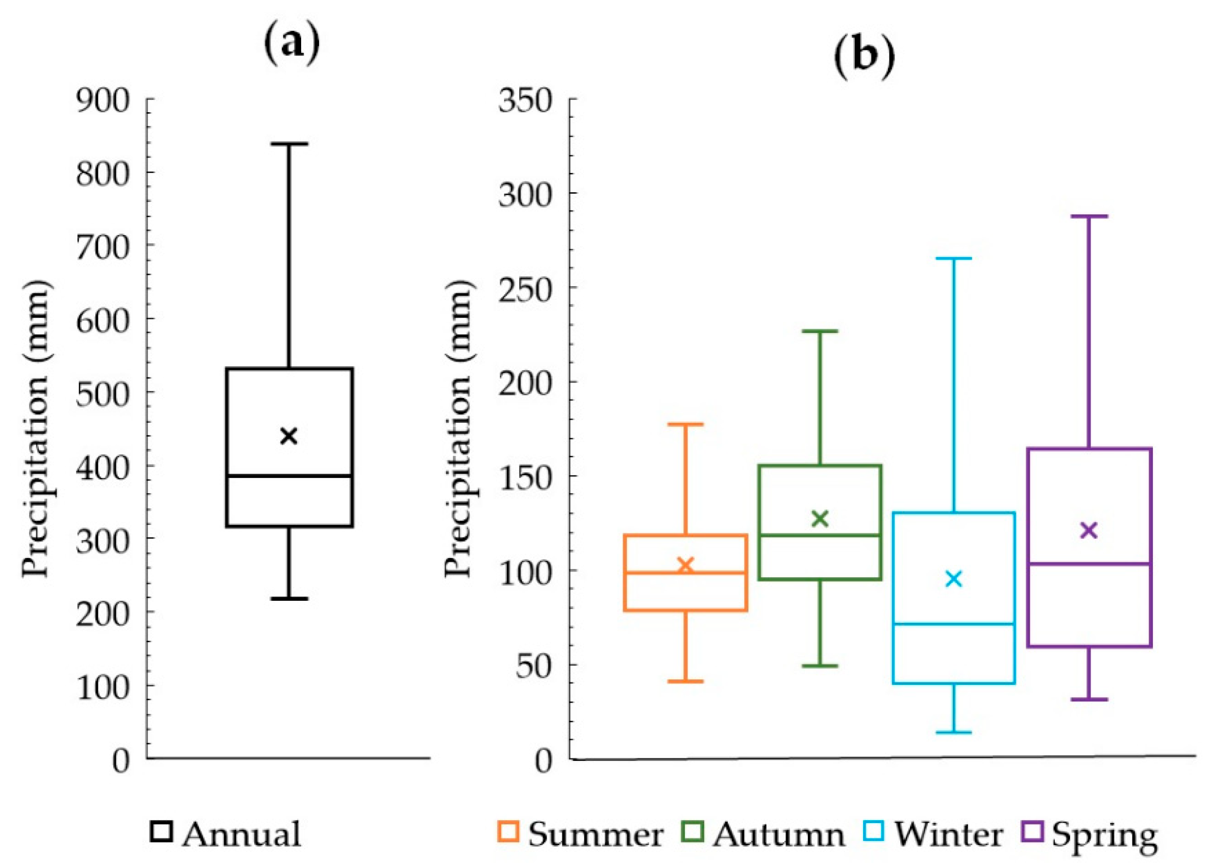
The total annual and seasonal total precipitation accumulation distribution are displayed in
Figure 5a,b, respectively, for the 1970–2019 period.
Figure 5b reveals the annual cycle of the precipitation with maximum (minimum) in autumn and spring (summer and winter) seasons. Similar behavior was reported by Turner et al. [
17] by analyzing the annual total precipitation days at the Faraday/Vernadsky station.
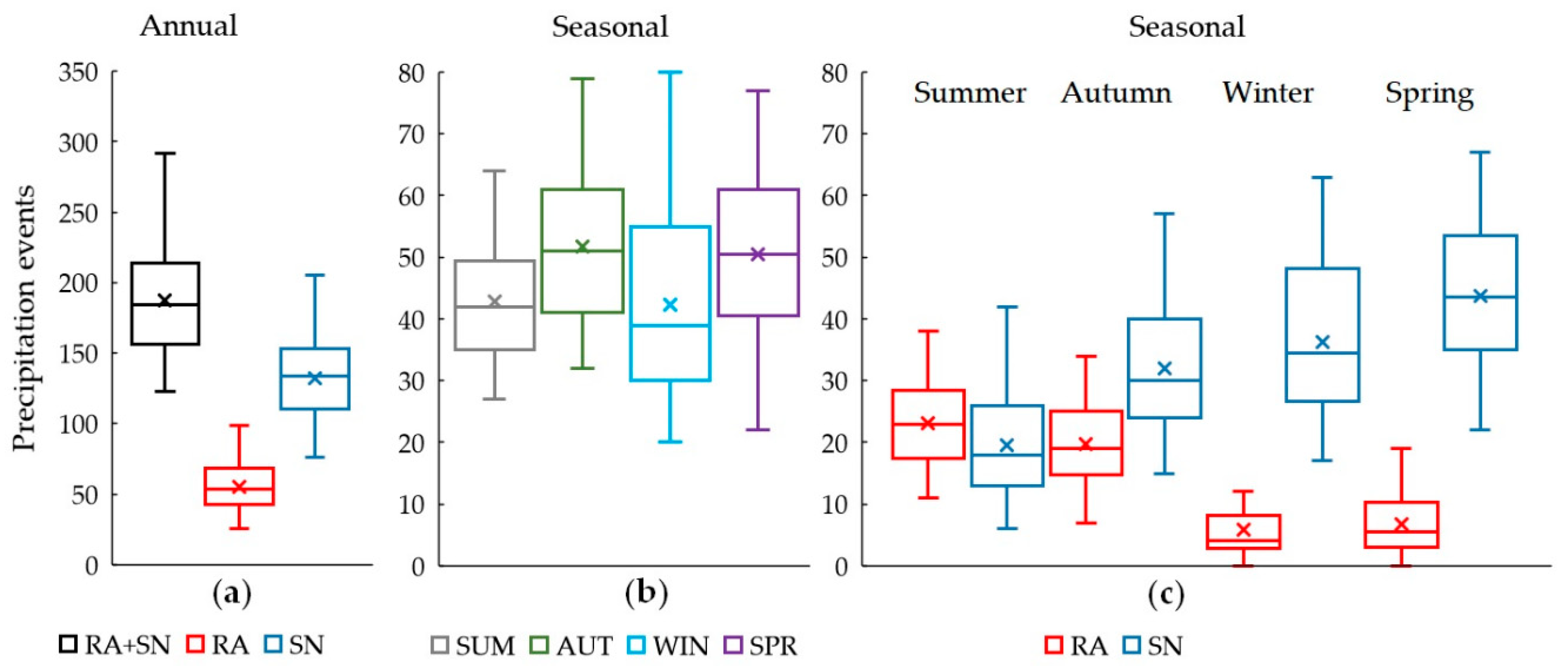
Figure 6 illustrates the annual and seasonal distribution of the type of precipitation as registered at Frei station (see also
Table 1). All liquid-precipitation events (DZ, RA, and RASH) were categorized as rain (RA), while all solid-precipitation events (SN, SNSH, RASN, and RASNSH) as snow (SN). The difference between the number of precipitation days and precipitation events is because the 3-hourly data sometimes registered snow and rain events and even drizzle events during the same day; here, each event was counted. On average, the annual number of snow events is three times larger than rain events (
Figure 6a), while the seasonal distribution of all precipitation events shows similar behavior to the precipitation days with maximum events during the equinoctial months. In addition,
Figure 6b reveals that rain mainly occurs during summer and autumn, and it is almost absent in winter and very scarce in spring. On average, the number of snow events is similar to the rain events (excluding DZ) during summer, and it is twice in autumn and largely superior during winter and spring seasons.
Table 1 shows the mean and standard deviation and the statistic parameters to analyze the statistical property of the time series. These statistic parameters are related to the normal distribution, and if so,
Cs and
Ck must be equal to 0 and 3, respectively [
18]. Generally speaking, if
Cs < 0.5, then the time series can be considered very symmetrically distributed, if
Ck > 0 (<0), then it indicates that the distribution is more (less) pointed, and if
Cv < 0.8, then it means that the data are homogeneous. On the other hand, if the DW test is closer to 2, then the time series is not autocorrelated (statistical significantly at
p < 0.05). If it is substantially below (above) 2 means that the data is positively (negatively) autocorrelated.
Examining the statistic parameters displayed in
Table 1, it is assumed that most of the analyzed time series were close to the normal distribution according to the
Cs parameter (except RA + SN annual and winter, SN summer, and RA winter and spring), and they are not autocorrelated (except RA summer) according to the DW test. SW test confirms the mentioned normal distribution but includes SN in winter, while the MK test indicates that the time series is homogeneous except for RA in annual and winter. On the other hand, the effective number
tbe confirms that most of the time series are nonautocorrelated. Therefore, the found linear trends are considered true tendencies, even so, Sen’s slope and the Kendall’s tau rank correlations (τ) were performed (Equations (11) and (12)) and indicated in each graph.
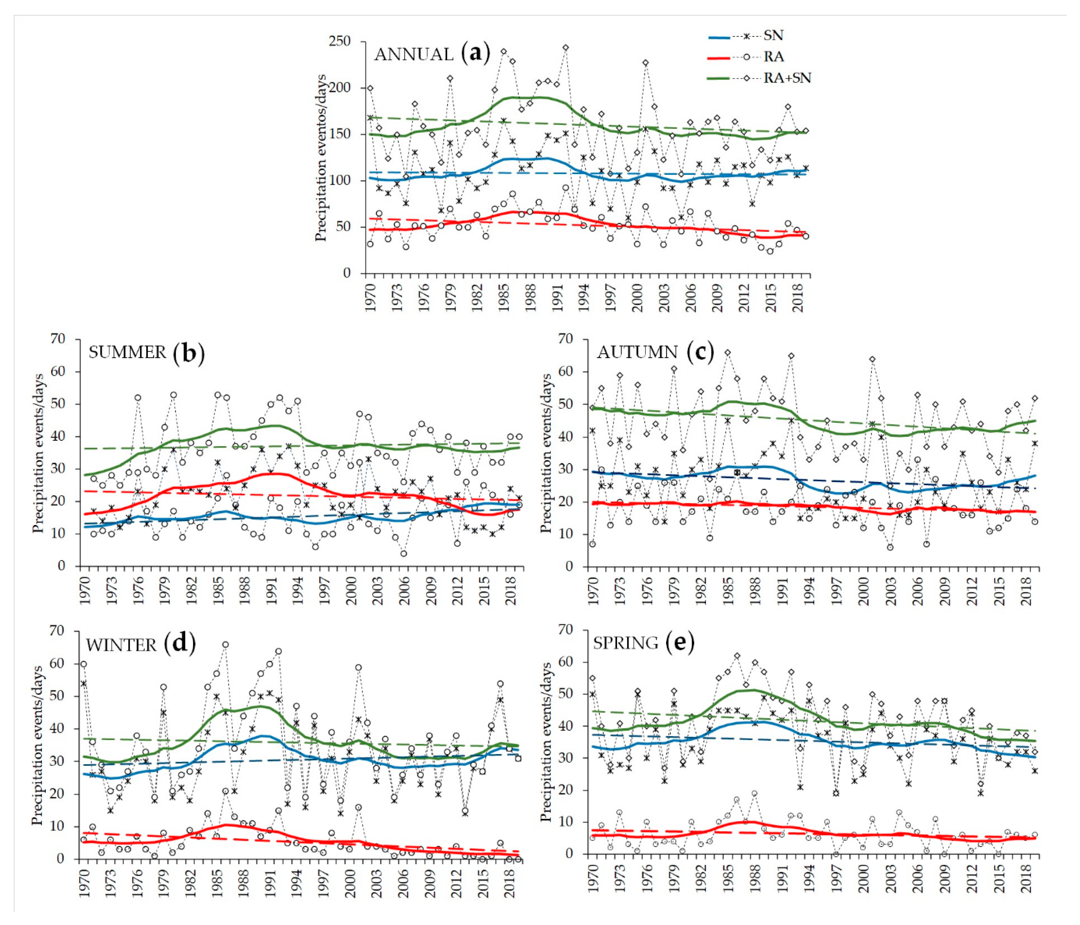
Figure 7 illustrates the annual and seasonal behavior of the rain/drizzle (RA) and snow (SN) events per day that took place at Frei station during the 1970–2019 period.
Table 2 shows the statistically significance of linear trends for all the precipitation events/day (RA + SN), and only for RA and SN of
Figure 7. The annual analysis reveals statistically significant (
p < 0.05) decreasing linear trends for the total number of RA+SN and RA events/day, and a nonsignificant slight increase for SN events/day. However, the decadal-like behavior revealed by the exponential filter shows an increasing period for RA + SN events from 1970 to mid-1980s (+26 ± 6 days (10 year)
−1,
p < 0.05) and a decreasing period from mid-1980s to 2019 (−13 ± 3 days dec
−1,
p < 0.05). These trends are also observed for the annual number of RA (+12 ± 2 days (10 year)
−1 (
p < 0.05) for 1970-mid-1980s and −9 ± 1 (10 year)
−1, (
p < 0.05) for mid-1980s-2019) and SN events (+13 ± 4 days (10 year)
−1 (
p < 0.05) for 1970-mid-1980s and −4 ± 3 days (10 year)
−1 (
n.s.) for mid-1980s–2019). The initial behavior (from 1970 to mid-1980s) is similar to the precipitation accumulation described previously (compared with
Figure 2 and
Figure 4) but differs from ~1991 to 2019 where the overall increase in annual precipitation, mainly from the mid-2000s onward, is accompanied by a negative trend in precipitation events.
The summer season shows an overall positive (
n.s.) trend of the RA + SN events due to the significant increase (
p < 0.05) of SN events, while during the autumn, winter, and spring seasons, the, respectively, overall negative trends are given by the decreasing SN and RA events except for winter that shows an increase in SN events. The exponential filter depicts the decadal-like behaviors of the precipitation changes. Therefore, the interannual and decadal-like seasonal variability reveals more complex changes in precipitation events. The summer season shows an overall increase of the RA + SN events (+8 ± 1 day (10 year)
−1,
p < 0.05) during 1970–1991 period and a nonsignificant trend after 2000. In this season, the RA events significantly increased from 1970 to 1991 (+8 ± 4 day (10 year)
−1,
p < 0.05) and decreased from 1992 onward (−5 ± 3 days (10 year)
−1,
p < 0.05), while the SN events show an overall increase for the 1970–2019 period. These changes are similar to the one found by Ding et al. [
19]. The decadal-like behavior for the autumn season reveals a statistically significant (22 ± 21 days (10 year)−
1,
p < 0.05) decreasing change during the 1990s but nonstatistically significant changes during the 21st century for RA + SN and SN events. RA events show an overall nonsignificant statistically decreasing trend during the 1970–2019 period (
Table 2). During the winter season, significant increasing trends of +9 ± 2 days (10 year)
−1 (
p < 0.05) and +7 ± 1 day (10 year)
−1 (
p < 0.05) for RA + SN and SN events, respectively, occurred from 1970 to 1992; and decreasing trends of −4 ± 5 days (10 year)
−1 (
p < 0.1) for RA + SN and −3 ± 4 days (10 year)
−1 (
p < 0.1) for SN events took place during the 1990s. While during the spring season, increasing trends (+8 ± 1 day (10 year)
−1,
p < 0.05 for RA+SN and +5 ± 1 day (10 year)
−1,
p < 0.05 for SN events) were obtained from 1970 to late-1980s and decreasing trends (−13 ± 1 day (10 year)
−1),
p < 0.05 for RA + SN and (−9 ± 1 day (10 year)
−1),
p < 0.05 for SN events occurred during the 1990s.
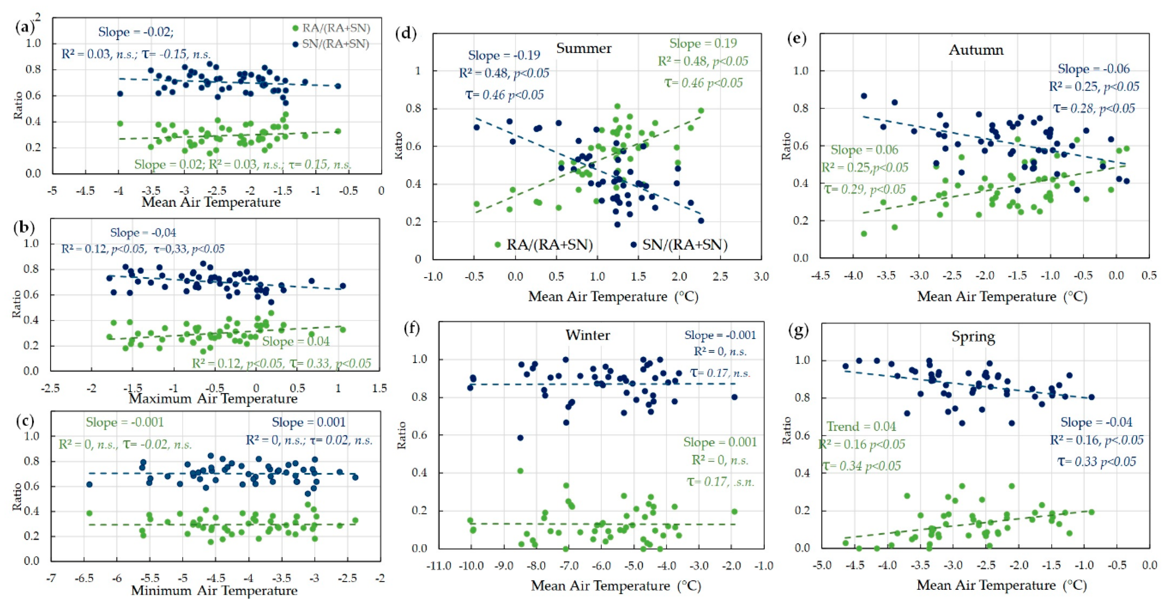
Figure 8 shows the annual and seasonal ratio between the rain (RA) and snow (SN) events with respect to the total (RA + SN). Overall, there is a significant correlation between the annual mean air temperatures and the RA/(RA + SN) and the SN/(RA + SN) ratios, being weaker for minimum temperatures and during the winter season. As air temperature increases (decreases), RA/(RA + SN) (SN/(RA + SN)) ratio increases (decreases). Annual analysis indicates that the changes in annual mean temperatures at Frei were able to explain up to 15% of the observed variability in the RA/(RA+SN) and SN/(RA + SN) ratios. Based on the trendline slopes, 1 °C increase (decrease) in the annual mean temperatures implies a ~2% increase (decrease) of the total percentage of precipitation that falls as rain (snow) with respect to the total precipitation events (RA + SN) (
Figure 8a). Changes in the average annual mean maximum temperatures at Frei were able to explain ~12–33% of the observed variability in the Ra/(RA + SN) and SN/(RA + SN) ratios, while the trendline slopes indicate that 1 °C increase (decrease) in the mean annual maximum temperatures was associated with ~4% increase (decrease) in the total percentage of precipitation that falls as rain (snow) with respect to the total precipitation events (RA + SN) (
Figure 8b). No changes occur associated with the observed variability in the RA/(RA + SN) and SN/(RA + SN) ratios and the average annual mean minimum temperatures (
Figure 8c).
The seasonal analysis indicates that in summer, the changes in the annual mean temperatures at Frei station can explain 46–48% of the observed variability of the RA/(RA + SN) and SN/(RA + SN) ratios. The trendline slopes, resolve that an increase (decrease) of 1 °C in the annual mean temperature was associated with ~19% of the increase (decrease) of the total percentage of precipitation that falls as rain (snow) to the total precipitation events (RA + SN) (
Figure 8d). In autumn, the changes in the average annual temperatures were able to explain ~25–29% of the observed variability in the RA/(RA + SN) and SN/(RA + SN) ratios. The trendline slopes indicate that 1 °C increase (decrease) in annual mean temperatures was associated with a ~6% of the increase (decrease) in the total percentage of precipitation that falls as rain (snow) to total precipitation events (RA + SN) (
Figure 8e). In winter, the changes in annual mean temperatures were able to explain up to ~17% of the observed variability in the SN/(RA + SN) ratio. The trendline slope resolved that decrease in annual mean temperatures was associated with a nonsignificant decrease in the percentage of total precipitation, which falls as snow to the percentage of total precipitation events (RA + SN) (
Figure 8f). Finally, in spring, changes in average annual temperatures explain ~16–34% of the observed variability in the RA/(RA + SN) and SN/(RA + SN) ratios, and the trendline slopes indicate that 1 °C increase (decrease) in annual mean temperatures was associated with a 4% of the increase (decrease) in the percentage of total precipitation that falls as rain (snow) with respect to the percentage of total precipitation events (RA + SN) (
Figure 8g).
4. Discussion
Precipitation analysis in windy and cold regions like in the AP is always accompanied by uncertainty due to blowing and drifting snow [
12]. Despite this restrained, available precipitation measurements can give some insides about changes that have been occurring in the northern tip of the AP. In this study, the overall annual behavior given by the linear trends of precipitation accumulation, precipitation days, and type of precipitation events were separated in periods of increasing and decreasing trends (decadal-like behavior) as revealed by applying the exponential filter (Equation (13)). Thus, increasing trends were found from 1970 to 1991 and from the mid-2000s to 2019, and a decreasing trend in between. This behavior of increasing and decreasing precipitation trends for 1970–1991 and early 1990-mid-2000 periods, respectively, concurs with the decadal snow accumulation (mm year
−1 w.eq. (water equivalent)) changes analyzed by Monaghan et al. [
9] and Monagham and Bromwich [
20], in the northern tip of the AP (see their
Figure 2,
Figure 3 and
Figure 4, respectively). Previous to 1970, precipitation in the northern AP has already been increasing as resolved by Turner et al. [
18] analyzing precipitation data from Faraday/Vernadsky station from 1958 to 2001 and by Monaghan et al. [
9] who derived snow accumulation by combining model simulation and observations from ice cores for Antarctica from mid-1950 to 2004. The seasonal analysis indicated that winter shows the larger significant increasing trend (
p < 0.05) followed by summer, but winter shows the same decadal-like changes than the one observed in the annual analysis.
The precipitation accumulation and precipitation days distribution revealed the annual and semiannual cycles of the precipitation with maximum (minimum) in autumn and spring (summer and winter) seasons This annual/semiannual cycle is associated with the annual/semiannual oscillation of the circumpolar trough that surrounds the Antarctic continent [
21,
22] and annual/semiannual and precipitation behavior in AP [
22]. This trough is deeper and closer to the continent in early autumn (March) and spring (September), indicating maximum cyclonic activity during these seasons. In addition, the meridional pressure differences between 50° and 70° S reach maximum during the autumn and spring seasons, being these changes related to the Southern Annular Mode (SAM, or Antarctic Annular Oscillation AAO) and therefore with the semiannual oscillation of the geostrophic winds of the lower troposphere [
23]. In other words, the strength of the westerly airflow, that prevails to the north of the circumpolar trough, is largely forced by the intensity of the trough [
22], resulting in more cyclonic activity during these seasons in the northern tip of the AP.
To get more insides of the precipitation changes, the datalog containing the type of precipitation was used. This gives us information about precipitation day and the type of precipitation at the time of the observation. The main results of this analysis are (1) the increasing and decreasing trends (statistically significant at
p < 0.05) in snow and rain events, respectively. Ding et al. [
19] (2020) have already indicated a clear shift in the type of precipitation days, with a significant decrease of total rain days and an increase of total snow days from 2001 until 2014 for the 1985–2014 period at the Great Wall station. This decadal-like behavior is similar to the one described here, although the amount of the average number of summer precipitation days, rain days, and snow days were around 22% larger than the ones computed here. This difference can be related to the high spatial variability and uncertainty in precipitation measurements in Antarctica, even in registering and categorizing the type of precipitation. At Frei station, e.g., snow depth less than 0.5 cm and light rain and drizzly with less than 0.1 mm are registered as trace (0.0), and in this study, only measurements ≥ 0.1 mm were considered. (2) Prevailing snow events were found during winter and spring, with significant decadal-like increasing (
p < 0.05) trend from 1970 to 1991 and a decreasing trend (
p < 0.05) from 1992 onward. Kirchgäßner [
24] analyzed the precipitation days at Faraday/Vernadsky station for the 1960–1999 period and found an annual increase in the number of precipitation days with the highest increase rates in winter and autumn, and she also found a significant positive trend (
p < 0.05) of precipitation events during winter. Here, for the 1970–1999 period at Frei station, the total number of precipitation events/day resulted in significant increasing trends in summer: 4 ± 2 days (10 year)
−1 p < 0.05, winter: 4 ± 2 days (10 year)
−1 p < 0.05, and spring: 2 ± 2 days (10 year)
−1 p < 0.05), whereas a decreasing trend in autumn (−2 ± 1 day (10 year)
−1 p < 0.05).
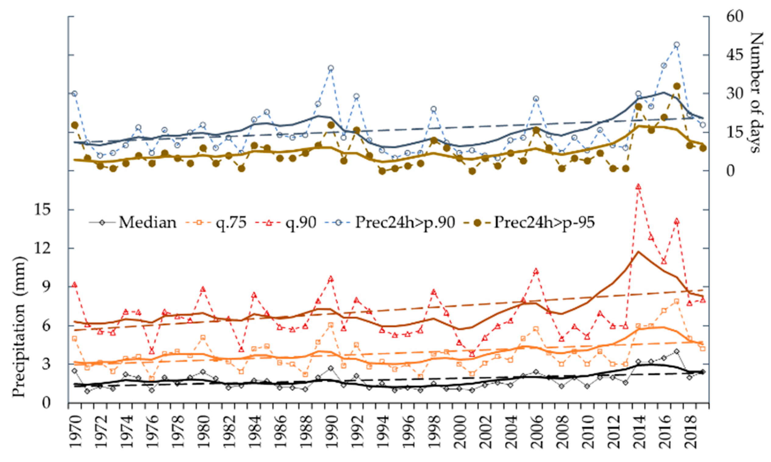
Even though using precipitation quantity needs to be interpreted with caution, the fact that the annual accumulation shows positive significant trends during the 1970–1991 and 2000–2019 periods, while the annual total number of precipitation event RA + SN that shows an overall decline from the early-1990s onward, need to be examined. For that, the median, the third quartile (about the first positive standard deviation), and the 0.9 percentile (considered the threshold for extreme events) were calculated for each year. In addition, the number of precipitation days (as given by the amount of precipitation accumulated in 24 h) above the 0.9 and 0.95 percentiles were computed. The results are depicted in
Figure 9. The overall significant positive trends (
p < 0.05) over the 1970–2019 period can be seen, but the exponential filter analysis reveals significant increasing trends (
p < 0.05) that occurred from 1970 to 1990 and from the late-1990s onward and a decreasing period between them (
n.s.). The increasing trend of these statistic parameters suggests that the reversal behavior between precipitation accumulation and the number of total precipitation events during the last period is associated with increasing extreme events.
The seasonal correlations between air temperature and the ratio of rain (RA) and snow (SN) event to total events (RA + SN) indicate that the largest changes in precipitation, as an increase (or decrease) in air temperature occurs during summer, whereas during winter, it can be considered nonsignificant (only 1% of the total precipitation events (RA + SN) (
Figure 8f).
Large-scale forcing factors that can influence precipitation in AP are the El Niño Southern Oscillation (ENSO), the Southern Antarctic Mode (SAM, or Antarctic Annular Mode (AAO), and the Amundsen Low Sea (ASL). The ASL is one of the climatological low-pressure centers located in the circumpolar trough in the southern Pacific Ocean centered around the Amundsen Sea and develops because of the large number of cyclonic depressions that moved southeastward from midlatitudes or developed in the baroclinic zone of the circumpolar trough [
25]. Guo et al. [
26] found an overall anticorrelation between the Southern Oscillation Index (SOI,
https://www.cpc.ncep.noaa.gov/data/indices/soi) and the precipitation in Marie Byrd Land, West Antarctica, and a positive correlation over the south Atlantic sector and in the northern tip of the AP (both statistically significant). This means that the negative ENSO phase (La Niña) can favor precipitation in the AP regions, while the positive phase (El Niño) can preclude it. On the other hand, the positive phase of SAM is associated with the strong polar vortex and southward displacement of the westerlies favoring precipitation in the AP [
27] and across much of West Antarctica and reduce the relatively small amount of precipitation over the Plateau [
28], while for the negative phase, the westerlies are displaced northward precluding precipitation. Additionally, studies have shown that the depth of the ASL is strongly influenced by SAM and ENSO modes [
27]. Thus, the positive SAM phase can favor the deepening of the ASL and the negative SAM phase its weakening [
27], while the ASL is weaker and displaced eastward during El Niño and deeper and displaced westward during La Niña [
27]. However, the difference between the actual values of the ASL pressure center and the area-average sea level pressure enclosing the ASL (over the sector 170–298° E and 60–80° S) [
29] gives the pressure gradient of the ASL, and therefore, its intensity. Nonstatistically significant tendencies were found in the annual and seasonal pressure gradient of the ASL, implying that nonintensification changes have occurred in the atmospheric circulation associated with the ASL during the 1979–2019 period. This concurs with Hosking et al. [
29] who stated that the SAM does not necessarily influence the strengthens of the ASL, but its longitudinal position does play an important role in defining the surface climate of West Antarctica and surrounding ocean areas. The overall annual longitudinal position of the ASL does not reveal any displacement during the 1979–2019 period. However, by analyzing the seasonal behavior, a westward displacement of about 6 ± 5 degrees (10 year)
−1 (
p < 0.05) was found during summer, an eastward displacement in winter of 4 ± 5 degrees (10 year)
−1 (
p < 0.05), slight significant westward displacements (less than 1 degree (10 year)−1) were found for autumn and spring.
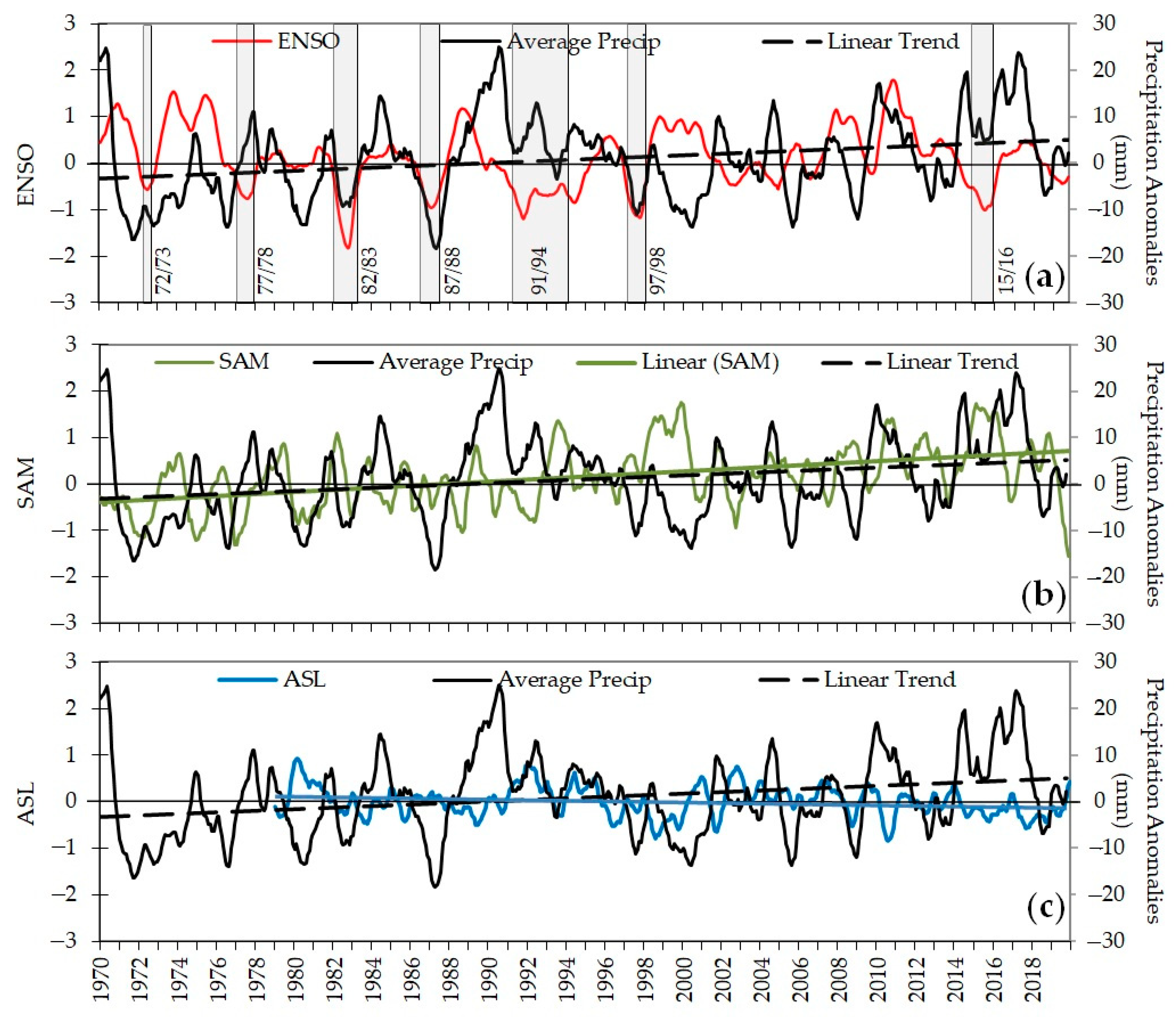
Figure 10 displays the monthly anomalies of the areal-average precipitation from the Chilean stations, along with the ENSO, SAM [
30,
31], and ASL indices [
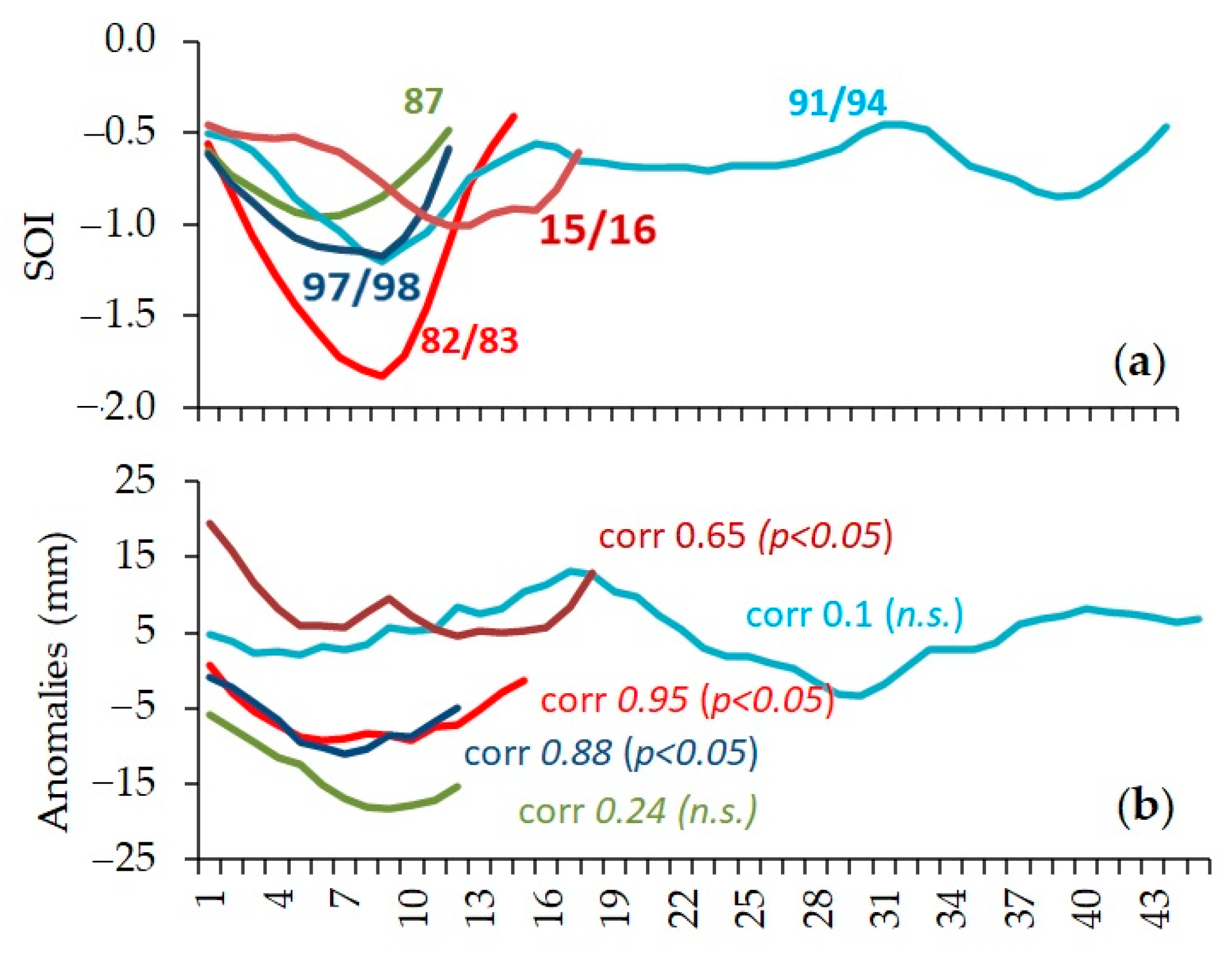
29]. All data were smoothed applying Equation (13) to filter out the high monthly variability. Nonstatistical correlations were found between monthly precipitation and each of the forcing factors. By examining each atmospheric index, only for moderate and strong El Niño events (1982/1983, 1987/1988, 1997/1998), the precipitation showed negative anomalies, and even for El Niño 2015/2016, a decreasing period occurred within the overall positive anomalies prevailing between 2014 and 2018 (
Figure 11). No correlation was found between individual La Niña events and precipitation [
32].
5. Conclusions
The available precipitation data from the Chilean weather stations located in the northern tip of the AP were used to analyze decadal-like changes during the 1970–2019 period. Moreover, at Frei station, where trained personal carry out weather observations, the precipitation type is registered at the time of the observation and now the data are available for analyzing precipitation phase (rain versus snow) year round. The exponential filter applied to the annual and seasonal precipitation data and on the forcing factors allows us to conduct a decadal-like analysis. Thus, the decadal-like changes in precipitation amount show a significant increasing trend (
p < 0.05) from 1970 to 1991, followed by a decreasing period (
p < 0.05) from the early-1990s to the early-2000s and an increasing trend hereafter (
p < 0.05). In addition, the annual precipitation events/days (RA + SN) depict the same behavior from 1970 to early-2000s but no increasing trend is resolved during the last decade, in fact, overall decreases were found for winter and spring seasons. This suggests that during the 2010s, an increase in extreme precipitation events has occurred, which is confirmed by the analysis of extreme events presented here (
Figure 10).
The overall positive trend of the SAM (
Figure 12) suggests the deepening of the ASL and therefore, more frequent synoptic-scale low-pressure systems moving southeastward that can favor the precipitation events in the northern tip of the AP. However, the increasing trend in precipitation was interrupted by a decreasing trend from the early-1990s to the early 2000s. The ENSO index (SOI) reveals that during the 1980s and 1990s, prevailed El Niño episodes, which implies a decrease in precipitation, although it also implies an eastward displacement of the ASL, favoring precipitation near the AP. The decreasing precipitation trend during the 1990s concurs with the extended El Niño 1991–1994 and the strong El Niño 1997/1998. The positive precipitation trend was resumed in the early-2000s. La Niña episodes have been prevailing from the early-2000s to mid-2010s implying overall increasing precipitation. However, also, it implies a westward displacement of the ASL, which can be related to the fact that the total annual number of precipitation days (events) did not increase during this period. This indicates that an increase in extreme events has been taking place, mainly during the last decade, as revealed by the 0.90 percentile analysis (
Figure 9), and with the overall intensification of the ASL of −0.28 hPa (10 year)
−1, (
p < 0.05), driving mainly by autumn (−0.71 hPa (10 year)
−1,
p < 0.05) and summer (−0.61 hPa (10 year)
−1,
p < 0.05) and then by winter (−0.31 hPa (10 year)
−1,
p < 0.05), but not during spring (+0.16 hPa (10 year)
−1,
p < 0.10).
During the summer season, the precipitation shows an increase in snow events along with a decrease in rain events from around the mid-1990s to mid-2010s. This opposite trend was attributed to the summer location of the ASL which, on average, was displaced eastward before 2001 and westward afterward. This westward drift could allow cold southerly wind over the western side of the AP [
33] favoring snow events. In fact, a cooling period has been reported from 1999 to mid-2010s [
34,
35,
36], indicating an overall cold environment affecting the AP region supporting snow events, in particular, a cooling period has been taking place during the summer as revealed by the annual mean temperature described by Carrasco et al. [
37].
Further analysis is required for a better understanding of the complex behavior of the precipitation in the AP region, mainly for getting insights to improve modeling simulations in the context of operational forecasting and climate change studies in polar regions.


