Physics-Based Simulations of Flow and Fire Development Downstream of a Canopy

Abstract

The behavior of a grassland fire propagating downstream of a forest canopy has been simulated numerically using the fully physics-based wildfire model FIRESTAR3D. This configuration reproduces quite accurately the situation encountered when a wildfire spreads from a forest to an open grassland, as can be the case in a fuel break or a clearing, or during a prescribed burning operation. One of the objectives of this study was to evaluate the impact of the presence of a canopy upstream of a grassfire, especially the modifications of the local wind conditions before and inside a clearing or a fuel break. The knowledge of this kind of information constitutes a major element in improving the safety conditions of forest managers and firefighters in charge of firefighting or prescribed burning operations in such configurations. Another objective was to study the behavior of the fire under realistic turbulent flow conditions, i.e., flow resulting from the interaction between an atmospheric boundary layer (ABL) with a surrounding canopy. Therefore, the study was divided into two phases. The first phase consisted of generating an ABL/canopy turbulent flow above a pine forest (10 m high, 200 m long) using periodic boundary conditions along the streamwise direction. Large Eddy Simulations (LES) were carried out for a sufficiently long time to achieve a quasi-fully developed turbulence. The second phase consisted of simulating the propagation of a surface fire through a grassland, bordered upstream by a forest section (having the same characteristics used for the first step), while imposing the turbulent flow obtained from the first step as a dynamic inlet condition to the domain. The simulations were carried out for a wind speed that ranged between 1 and 12 m/s; these values have allowed the simulations to cover the two regimes of propagation of surfaces fires, namely plume-dominated and wind-driven fires.

1. Introduction

Every summer wildfire-prone countries brace for another devastating fire season. In recent years, the frequency of mega-fires has increased. For example, within a decade of the 2009 Black Saturday wildfire in Australia, the world witnessed the Black Summer of 2019–2020 in Australia. While there is debate on whether climate change or forest management is the more important contributing factor, the economic, ecological, and health consequences of these wildfires are huge [1]. Climate change and weather patterns occur at global scale and over a long period of time, resulting in protracted periods of drought, fuel dryness, and atmospheric conditions conducive to large fires. Whereas fire agencies can often manage forest growth or fuel abundance at local or regional settings, especially in wildland urban interfaces or near transitions from forest to grassland. Therefore, it is important to study the effect of forest structure on surface fires as a potential trigger to fires transitioning to an intense and fast-moving crown fire.

Additionally, as observed in many dramatic fire events, crown fires, generally characterized by a high intensity and therefore a strong convective plume, contribute to the increased emission rate of burning particles (brands), such as leaves or small piece of bark. Due to the mechanical action of the strong convective plume observed in these conditions, these burning particles (spots) can be transported over long distances (few kilometers) and can ignite many secondary fires ahead of the main fire front. This mode of propagation, called fire spotting, is considered to be a major source of fire hazard in the wildland urban interface (WUI). Because a clearing or a fuel break contributes in reducing the fire intensity, it also constitutes a means of reducing brands emission, which justifies the interest to study such configurations.

The driving wind velocity is an important parameter for the spread rate of a wildfire. The wind may be in an open grass field or through a forest canopy. Wind velocity profiles are changed within the forest canopy and also at the interface of forest and open-field, and consequently, affect the rate of spread (RoS). A forest-canopy exerts an aerodynamic drag force, and as a result, the wind speed is reduced. The shape of the canopy leaf-area-density (LAD) profile (which changes with height inside the canopy) determines the shape of the sub-canopy wind profile. In turn, the surface fire is somewhat sheltered within the forest canopy and exposed to slower winds [2]. Fire behavior analysts operationally model the effect of the sub-canopy wind-profile by using a Wind Reduction Factor (WRF), as exemplified by the McArthur model used in Australia [3]. Similarly, in the United States, a Wind Adjustment Factor (WAF) is used [4].

Natural plants often display regularities in their shapes. For example, the diameters of branches of a tree follow a well-defined distribution, which means that we are able to define the geometry of a tree. This enables researchers to estimate the drag coefficients, and as a result, it is possible to numerically predict the velocity profiles of the wind through some types of vegetation. There have been experimental and numerical studies to understand sub-canopy wind behavior [2,5,6,7,8,9,10] both deep within a canopy and near canopy edges. Cassiani et al. [5] explored the flow characteristics of the downstream edge region in detail and found that for dense canopies, a mean recirculation region was established similar to flow over a backward-facing step. Far away from the canopy, the flow can become similar to an open field wind profile. However, studies of fire propagation through forest canopies or downstream of the edges of a forest canopy are rare—the only known study is Sutherland et al. [11]. Without such studies, it is difficult to quantify the actual effect of the presence of forest canopy on the RoS. Experimental studies of this effect involving fire are often prohibitive due to safety concerns, expense and uncontrolled interaction of multiple physical and chemical phenomena. However, this configuration is particularly interesting from a practical point of view, because it can be encountered quite frequently during prescribed burning operations.

Physics-based models are able to conduct controlled numerical experiments with a good degree of fidelity. The information gleaned from the simulations can then be used to obtain insight into the mechanisms of fire spread. In the last decade or so, due to dramatic improvement in computational power, three-dimensional physics-based simulations with LES-based turbulence model have become a frequently used model of fire spread. FIRESTAR is one such model, which emerged from a two-dimensional model [12] and evolved into a three-dimensional one [13]. FIRESTAR3D is based on a multi-phase formulation and solves the conservation equations of the coupled system formed by the vegetation and the surrounding gaseous medium. The model takes into account the vegetation degradation processes (drying, pyrolysis, and combustion), the interaction between the atmospheric boundary layer and vegetation (aerodynamic drag, heat transfer by convection and radiation, and mass transfer), and the transport in the gaseous phase (convection, turbulence, and combustion). In this study, FIRESTAR3D is first used to conduct large eddy simulations of the flow through and over a plant canopy with different wind speeds and canopy densities. This phase was carried out as a precursor step in order to recover the flow conditions upstream of the grassfire considered in the second phase. For grassfire propagation, one canopy density with different driving wind velocities was studied. The objectives of this paper are (1) to study the flow redevelopment downstream of a tree canopy, (2) to characterize the RoS and the fire intensity of an idealized surface fire downstream of a canopy, and (3) to quantify the effect of the canopy on the RoS and the fire intensity.

2. Problem Description and Methodology

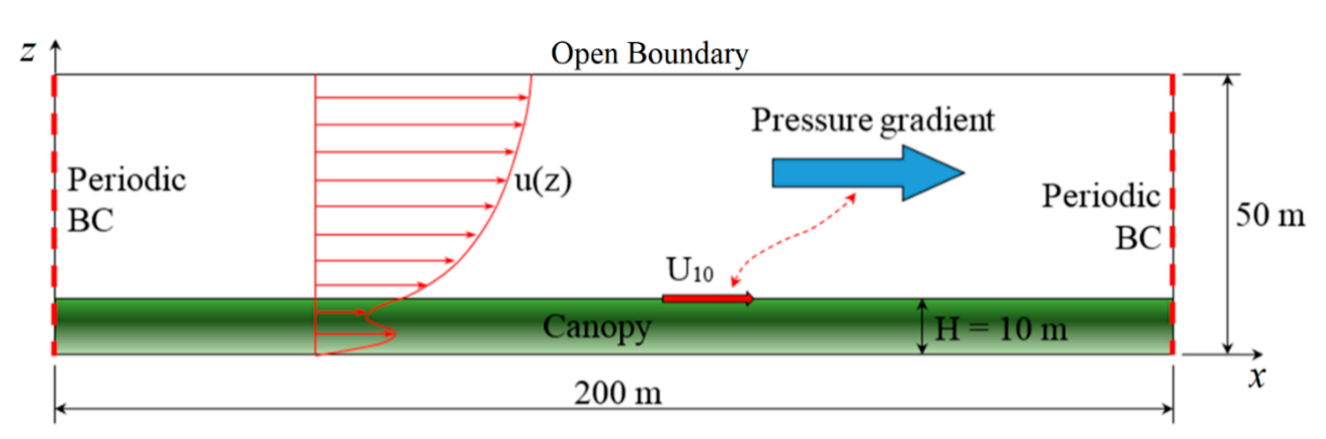
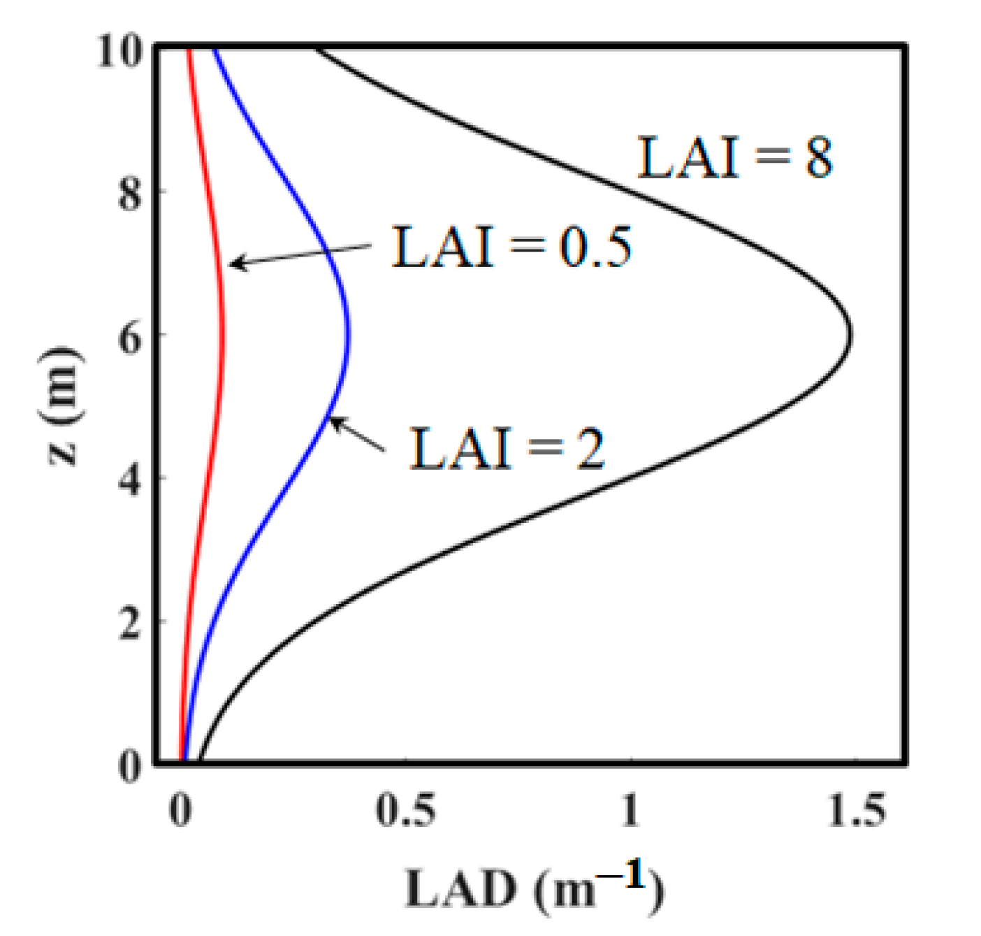
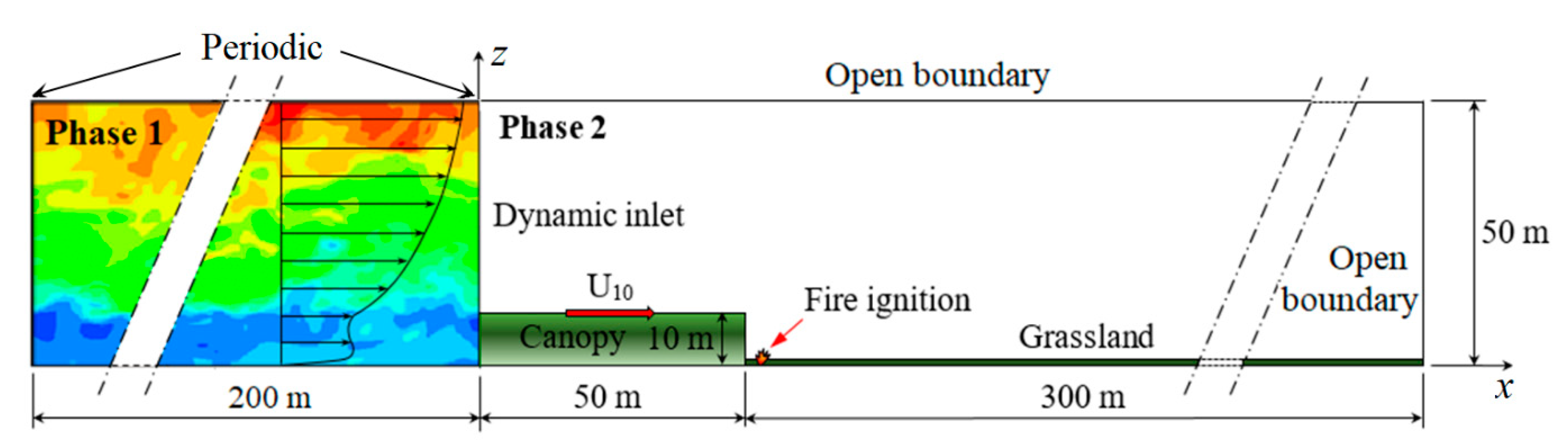
2.1. Problem Description and Approach

To study grassland fire-spread downstream of a canopy, we assumed that the canopy was sufficiently long that a well-developed sub canopy flow existed within the canopy, before the canopy exit. Flow development within a canopy typically requires a development length of 15 times the canopy height [7,8]. If a long distance downstream of the canopy is also required to simulate fire development, the computational domain may become prohibitively large. Therefore, to mitigate these computational difficulties, a short canopy was adopted for the fire simulations, and the inlet condition were chosen to be a well-developed canopy flow obtained from a precursor simulation. The precursor simulation is referred to as “phase 1” and the fire simulation is referred to as “phase 2.” The simulations in phase 1 aimed to produce a statistically-stationary canopy flow free from any edge effects, which is achieved by simulating the flow over the modeled tree canopy with periodic boundary conditions in the streamwise and spanwise directions as in [14]. The flow obtained from this precursor phase was then applied at the inlet of the computational domain upstream the grassland fire, considered in phase 2.

As shown by Figure 1, the computational domain used to perform the simulations in the first phase was 200 m long, 50 m wide, and 50 m high, with periodic boundary conditions applied in the lateral directions. Neumann conditions were imposed at the top of the computational domain, while the bottom boundary was considered to be a solid wall. The canopy was 10 m high, with an LAD that varies in the z-direction. The LAD defines the ratio of the total leaf area to the occupied foliage volume. The LAD can be evaluated from product α_Sσ_S, where α_S is the volume fraction of the solid particles and σ_S is their surface-to-volume ratio. σ_S was set to 4000 m⁻¹ and the required distribution of the LAD was obtained from a variable space-distribution of α_S. The distribution of the LAD in the vertical z-direction is given by Equation (1), which is representative of Australian pine canopies [5]:

$$\mathrm{LAD}={\mathrm{LAD}}_{\max }{e}^{-0.1{\left(z-6\right)}^2}$$

(1)

The maximum of LAD occurs at z = 6 m and its value LAD_max was determined in order to obtain the desired leaf-area-index (LAI), equal to the integral of LAD with respect to z over the canopy height H [15]. As shown by Figure 2, three values of LAI (0.5, 2, and 8) were considered in the first phase of the study. These values of LAI were chosen because they cover the transition of the flow over a canopy from a boundary-layer-like flow to a mixing-layer-like one, as shown by Nepf et al. [16]. This transition occurs for C_D × LAI ≈ 0.1 [16], where C_D is the drag coefficient of the canopy, equal to 0.15 [5] in this case.

The initial vertical distribution of the streamwise velocity used to start the simulations, corresponded to the steady-state velocity field obtained in the case of a constant-LAD plant canopy [17]. A random perturbation of 0.1 m/s amplitude was added to the initial velocity profile to accelerate turbulence development. A pressure gradient in the streamwise direction was applied to the x-momentum equation, and was dynamically modulated in order to reach the desired value of the average wind speed U₁₀ at the top of the canopy. The value of the pressure gradient tends asymptotically to zero once a statistically-steady flow is obtained. For each of the three values of the LAI reported in this study, five different values of U₁₀ were considered: 1, 3, 5, 8, and 12 m/s. Thus, a total of 15 simulations were carried out until a statistically-steady flow was obtained in each case. The development of the turbulent flow during this precursory phase was examined by considering the average profiles of turbulence statistics [14]. The steady state was considered to be reached when the average profiles of turbulence statistics and the mean stream-wise velocity at the top of the canopy were constant in time.

The turbulent flow obtained from this first precursor phase was used in the second phase to study the grassland fire-spread downstream of a plant canopy. As shown by Figure 3, the computational domain used to perform the simulations of the second phase was 350 m long, 50 m wide, and 50 m high. This domain consists of a 50-m-long canopy section that had the same characteristics as in phase 1. Periodic conditions were applied on the vertical-lateral boundaries to simulate a quasi-infinite fire-front [18,19]. The flow properties (velocity components, pressure, sub-grid kinetic energy) obtained at the statistically-steady state in phase 1 were applied as dynamic inlet (Dirichlet) conditions at the computational domain entrance. The use of such a time-dependent inlet boundary-condition was the only way to inject at the domain entrance the coherent structures resulting from an ABL flow through a quasi-infinite plant canopy (obtained from phase 1). The grassland downstream of the canopy was 300 m long, 50 m wide, and had the following main properties [13,20]: vegetation height h = 0.7 m, fuel volume-fraction α_S = 0.002, surface-to-volume ratio σ_S = 4000 m⁻¹, dry-material density ρ_S = 500 kg/m³, moisture content M = 5%, solid-fuel particles were assumed to have cylindrical shape and to behave as a black body. The second-phase simulations were carried out for a canopy LAI = 2 only (for reasons explained in the result section) and for the five values of U₁₀ considered in phase 1, i.e., U₁₀ = 1, 3, 5, 8, and 12 m/s.

The average-vertical profiles of the streamwise velocity and of the sub-grid kinetic energy obtained at statistically-steady state in phase 1 were used to initialize the simulations in phase 2. As in phase 1, the hydrodynamic module of FIRESTAR3D was run long enough in phase 2 for the flow to reach a statistically-steady turbulent flow downstream the canopy (again, this step is detailed in the results section). Once the flow had reached a statistically-steady state, the burner was activated uniformly between x = 53 m and x = 55 m along the entire domain width. Ignition was obtained by injecting CO gas at 1600 K in the burning zone (53 m < x < 55 m) from the bottom boundary of the domain. The burner was activated for 20 s (at most) or until the consumption of a solid-fuel mass equal to that available above the burning area (i.e., contained in a volume of 2 × 50 × h m³). When the burner was activated, the average velocity of CO injection was at its maximum (equal to 0.1 m/s), and then it was decreased linearly with the consumed mass of solid-fuel. This procedure avoids destabilizing the flame front by abruptly ceasing the CO injection and avoids any excessive external energy input. More details about the ignition procedure are given in [18,20].

Before fire ignition, the flow redevelopment distance downstream of the canopy was examined for the different wind speeds. After fire ignition, the fire regime, the RoS, and the fire intensity were reported at different positions downstream of the canopy. Finally, the effect of the canopy was examined by comparing the values of RoS and of the fireline intensity obtained, with and without canopy, for the same grassland properties. For this purpose, all the simulations (both phase 1 and phase 2) were exactly repeated while setting the canopy LAI to zero. The numerical simulations have been conducted using implemented FIRESTAR3D model.

2.2. Mathematical Model

FIRESTAR3D is a fully physics-based wildfire model [21] based on a multiphase formulation approach [22]. The details of the model have been widely presented in previous publications [12,20,21,23,24], and the most detailed description of FIRESTAR3D model can be found in [21]. The model consists of two parts that are solved on two distinct grids. The first part consists of the equations of a reacting-turbulent flow in the gaseous phase composed as a mixture of fresh air with the gaseous products resulting from the degradation of the solid phase (by drying, pyrolysis, and heterogeneous combustion) and the homogeneous combustion in the flaming zone. The second part consists of the equations governing the state and the composition of the solid phase subjected to an intense heat flux coming from the flaming zone.

Solving the gaseous-phase model consists in the resolution of conservation equations of mass, momentum, energy (in enthalpy formulation), and chemical species (O₂, N₂, CO, CO₂, and H₂O) filtered in space using a LES approach, with a Favre-average formulation [25]. The closure of the filtered conservation equations is based on the eddy viscosity concept [26]. An LES high-order sub-grid scale stresses model was used [27]. The temperature dependence of the gas-mixture enthalpy is based on CHEMKIN thermodynamic tables [28]. A combustion model based on the Eddy Dissipation Concept (EDC) was used to evaluate the combustion rate occurring in the gaseous phase [26,29]. The soot volume-fraction in the gas mixture is calculated by solving a transport equation including a thermophoretic contribution in the convective term and taking into consideration soot oxidation [30,31,32].

Concerning the solid-phase model, during the thermal degradation, the solid fuel particles are represented as a mixture of dry material (generic term for a mixing of cellulose, hemicellulose, and lignin), charcoal, moisture, and residual ashes. For each solid particle, the model consists in solving the equations governing the time evolutions of the mass fractions of water, of dry material, and of charcoal, as well as of the total mass of the solid particle, its volume fraction, and its temperature. The degradation of the vegetation is governed by three temperature-dependent mechanisms: drying, pyrolysis, and charcoal combustion [21]. The constants of the model associated with the charcoal combustion are evaluated empirically from a thermal analysis conducted on various solid fuels samples [22,33].

The interaction between the gaseous phase and the solid phase is taken into account through coupling terms that appear in both parts of the model. These terms are linearly interpolated between the fluid-phase and solid-phase grids. The coupling in the momentum and turbulence equations is obtained by adding aerodynamic drag terms [24]. Heat transfer between the gas mixture and the solid fuel is based on empirical correlations for convective-transfer coefficient [33], and on the resolution of the radiative-transfer equation [34] that accounts for the presence of soot in the flaming zone and for the presence of hot particles in the vegetation layer (embers) [22]. Finally, mass transfer from the solid phase to the gaseous phase is represented by adding source/sink terms in the mass conservation equations of both phases.

2.3. Numerical Method

The balance equations in the gaseous phase are solved numerically using a fully-implicit finite volume method in a segregated formulation [35,36]. FIRESTAR3D model predicts turbulent-reacting flows in rectangular domains using a structured but non-uniform staggered mesh. Time discretization relies on a third-order Euler scheme with variable time-stepping strategy. Space discretization is based on second-order schemes with flux limiters (QUICK scheme [36,37]) for convective terms, while diffusion terms are approached with a central difference approximation with deferred corrections [38]. The Radiative Transport Equation (RTE) is solved using a Discrete Ordinate Method (S8 approximation is often used) [39]. The RTE accounts for gas-soot mixture absorption of radiative intensity depending on the amounts of combustion products (CO₂ and H₂O), on the gas mixture temperature, and of the soot volume fraction [40]. The set of ordinary differential equations describing the time evolution of solid-fuel state (mass, temperature, and composition) are solved separately using a fourth order Runge–Kutta method. From an implementation point of view, the computation code is parallelized using OpenMP directives [41] and optimized [42,43]. Finally, the hydrodynamic module of the code has been extensively validated on several benchmarks of laminar and turbulent natural-convection, forced convection, and neutrally-stratified flow within and above a sparse forest-canopy [14,15,44,45]. The predictive potential of FIRESTAR3D model has been estimated at small scale in the case of litter fires in well-controlled experimental conditions (fire propagation through a homogeneous fuel-bed in a wind tunnel) [18,21] and at a larger scale for grassland fires (experimental campaign carried out in Australia) [13].

All simulations presented in this study were obtained using a variable time-step strategy based on the truncation-error control, with time step values varying between 0.001 s and 0.05 s. At each time step, the solution was assumed to be obtained when the residuals of all conservation equations had reached 10⁻⁴ in normalized form [21]. As a rough estimation of the computational cost in phase 2 (much higher than in phase 1), the simulation of 1s of fire propagation required about 7 h of CPU time on a 24-core node.

3. Results and Discussion

As detailed in Section 2, the study grassland fire-spread downstream of a canopy requires a precursor phase whose objective is to generate an ABL/canopy turbulent flow above a canopy using periodic boundary conditions along the streamwise direction. The simulations of this phase were carried out for a sufficiently long time to achieve a quasi-fully developed turbulence. The flow obtained from this precursor phase was then applied as a dynamic inlet condition at the entrance of the computational domain upstream the grassland in the simulations carried out in phase 2. Additionally, the same simulations were carried out without a canopy, in order to evaluate the effect of the canopy on the RoS and on the fire intensity.

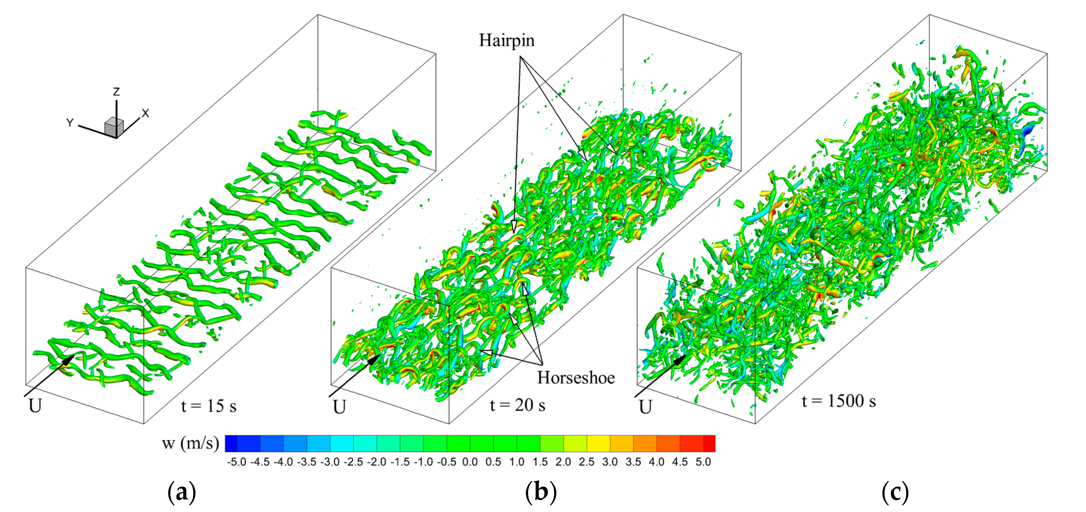
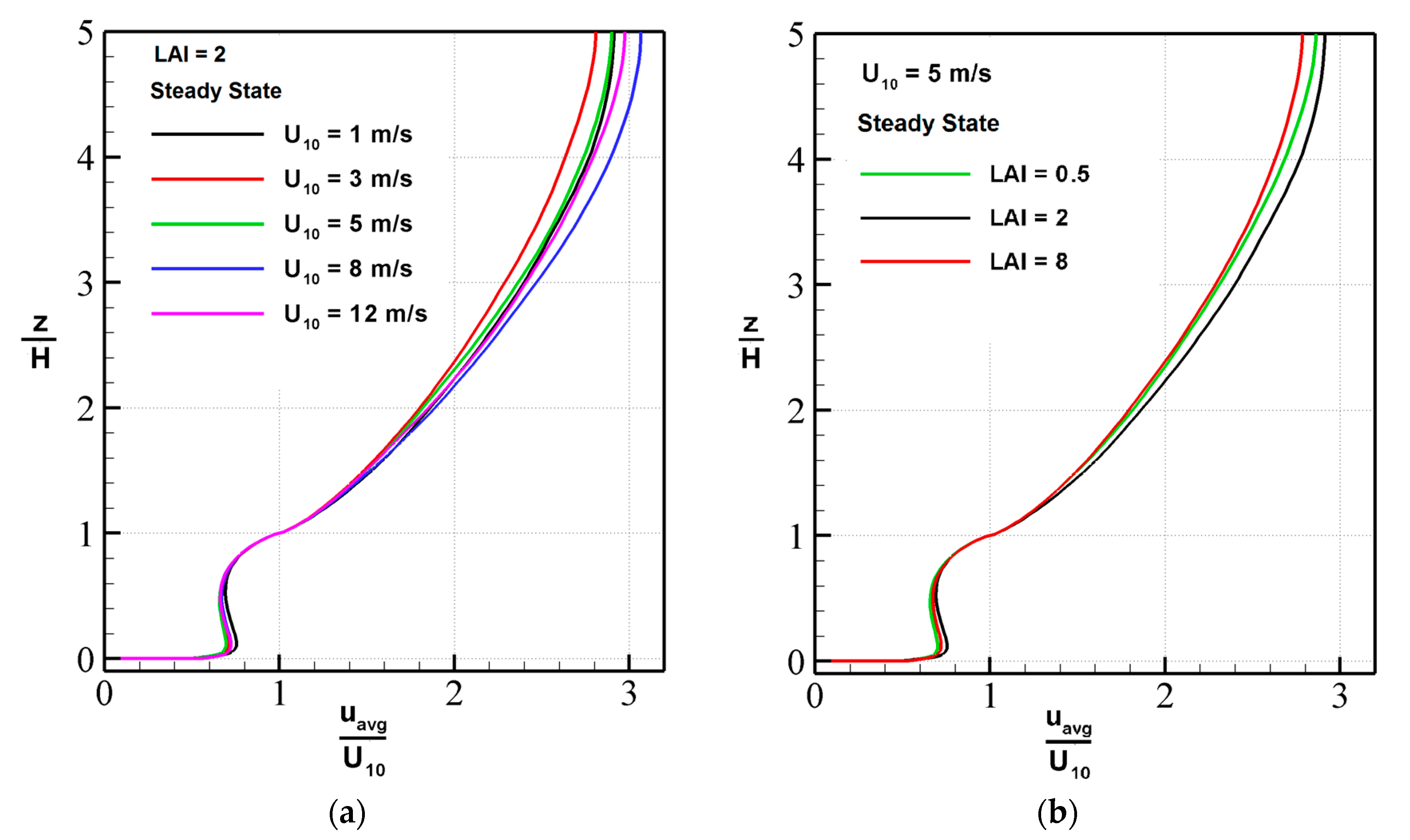
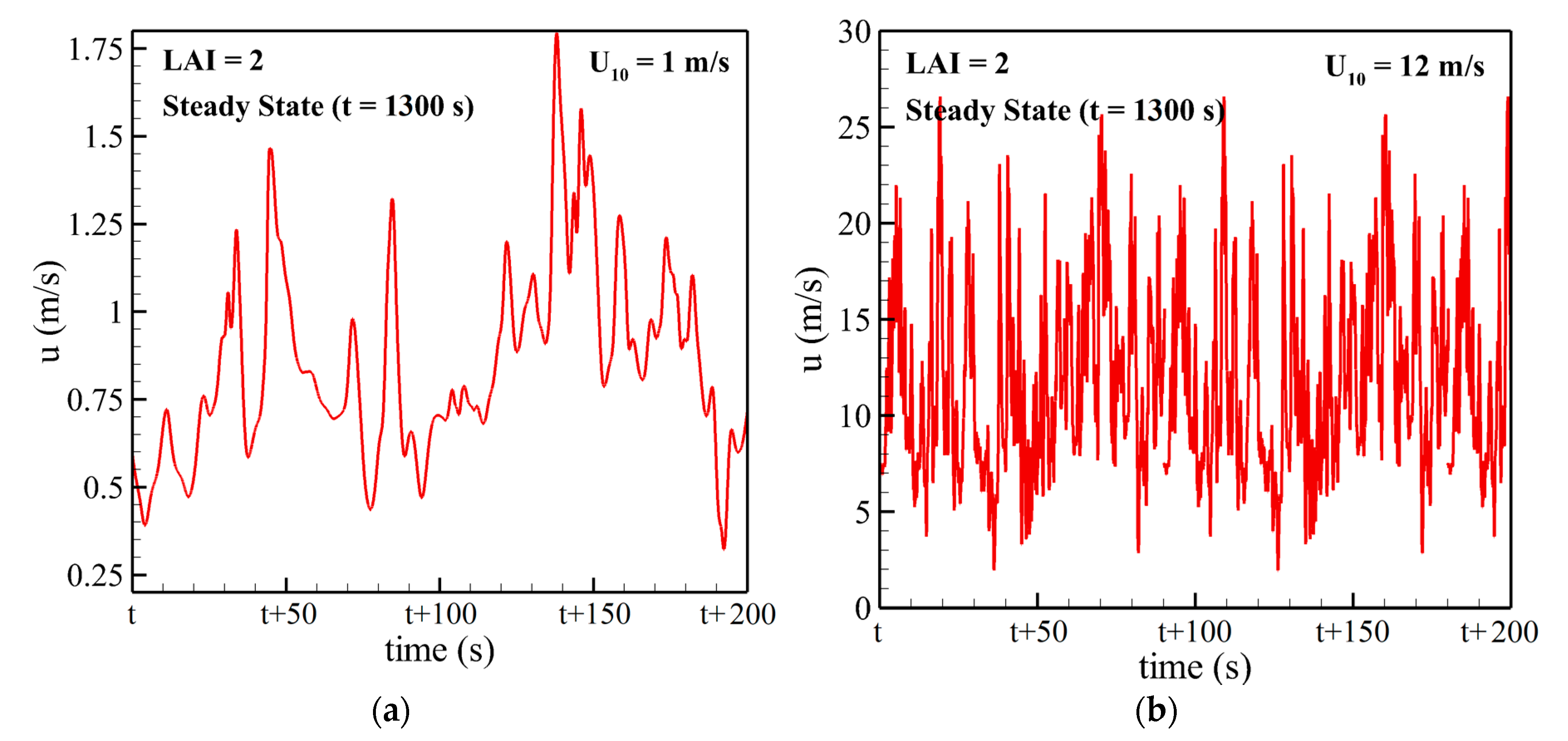
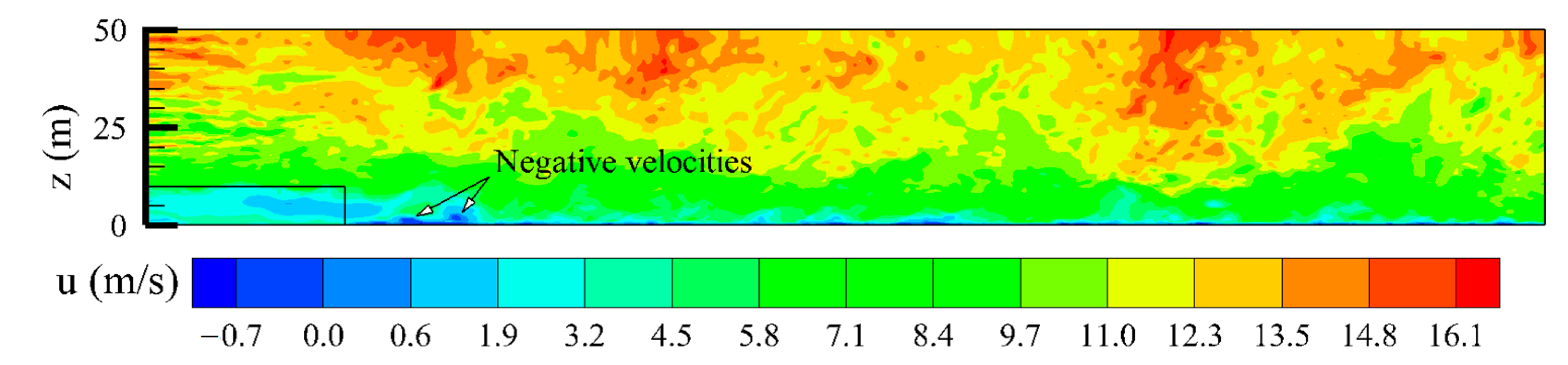
3.1. Phase 1: ABL Flow Over a Tree Canopy

The flow over a tree canopy has been extensively studied theoretically [9,46] and numerically [5,6,7,8,10,14]. We investigate the development of the turbulent the sub-canopy and above-canopy flow to confirm that our model correctly reproduces a well-developed canopy flow. The pathway to a fully turbulent over a tree canopy was described by Finnigan (2000) [46]. The first stage is the development of a Kelvin-Helmholtz instability and the formation of large-scale roller structures above the canopy. To visualize the vortex structures, we plot isosurfaces of the Q-criterion introduced by Hunt et al. [47]. The Q-criterion is the second invariant of the velocity-tensor gradient; however, the Q-criterion is more easily thought of as a difference between the squares of local vorticity and strain rate. A positive Q-criterion then indicates local dominance of the rotation component over the stretching component. The large-scale Kelvin-Helmholtz rolls are clearly visualized by the iso-surfaces of the Q-criterion in Figure 4a obtained for U₁₀ = 5 m/s and LAI = 2. The Kelvin-Helmholtz rolls come in pair in shear flows, where the vortices rotate around each other and eventually merge, due to the velocity induction mechanism: each vortex tends to lead the other non-rotational motions, causing the vortices to roll up around each other as shown in Figure 4b. Consequently, the outer part of each vortex turns more slowly than the inner part, and each vortex develops a tail leading to the development of so-called horseshoe vortices; some of these structures can be seen in Figure 4b. Then, longitudinal-hairpin vortices form by the stretching, by the ambient deformation field at the canopy-top level, of the weak vorticity that exists initially in the stagnation region between the Kelvin–Helmholtz rolls; the hairpin structures are also visible in Figure 4b. Finally, the fully-developed turbulent flow shown in Figure 4c is characterized by a dominance of streamwise vortices that are located at the top of the canopy. The progression shown in Figure 4 is in qualitative agreement with the mechanisms discussed by Finnigan [46]. Notice that in the case of Figure 4, C_D × LAI = 0.3 is three times the threshold value of 0.1 characterizing the transition of the flow over a canopy from a boundary-layer-like flow to a mixing-layer-like one [16]. Even though the explored flow contains characteristics of both flow types [14], the analogy with the mixing-layer flow is stronger: the presence of Kelvin–Helmholtz rolls pairing, three-dimensional helical pairing, and hairpin vortices suggests more similarity with a mixing-layer flow transition.

Primarily, the RoS is related to the mean u-velocity, and most empirical models (e.g., [3,4]) rely on estimates of mean u-velocity as an independent variable. To investigate the modification of the u-velocity as a function of height with the imposed canopy-top velocity and LAI, normalized profiles are plotted in Figure 5. These profiles, averaged between 1200 s and 1500 s (i.e., after the flow has achieved a statistically-stationary state) and in the streamwise and spanwise directions, are normalized by the canopy-top velocity. The normalized sub-canopy profiles show almost no variation with canopy-top u-velocity and LAI when the average wind speed is imposed on the canopy surface. However, a stronger streamwise pressure gradient is required of course to maintain the desired flow speed as the canopy LAI and canopy-top u-velocity are increased.

The variation of the u-velocity at the canopy surface over time is shown in Figure 6 for U₁₀ = 1 m/s and 12 m/s velocity cases. The u-velocity oscillates around a constant mean, showing the flow is well developed, and we noticed that the wind speed increases the frequency of fluctuation of the velocity. Interesting analyses may be conducted for the ABL flow over a tree canopy, such as characterizing the wavelength and the frequency contents of the velocity field, but this would be tangential to the main objective of the paper, which is to study the spread of a grassland fire downstream of a canopy.

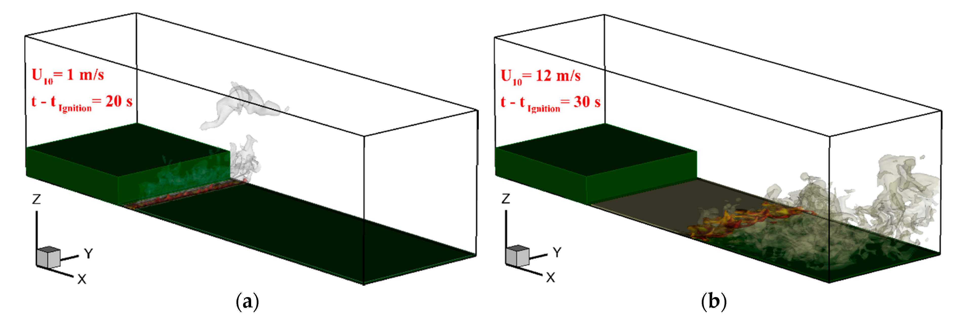
3.2. Phase 2: Grassland Fire Spread Downstream of a Tree Canopy

For phase 2, the phase 1 simulations were applied as a dynamic inlet condition on the upstream boundary. The flow was then allowed to evolve to a statistically-stationary state, where the mean flow is constant in time. Allowing the flow to evolve for 1000 s of simulated time was found to be sufficient for all considered wind speeds to give a well-developed velocity field downstream of the canopy before fire ignition. We chose to simulate fire spread for only LAI = 2. Firstly, the canopy LAI has no significant effect on the normalized average sub-canopy velocity profile (as shown by Figure 5) when the wind speed is imposed on the canopy surface; thus, this LAI is representative of a wide range of flows. In addition, this LAI value and LAD profile adopted are also representative of a reasonable range of forests prone to bushfires, see for example measurements in Amiro [48] and Moon et al. [2].

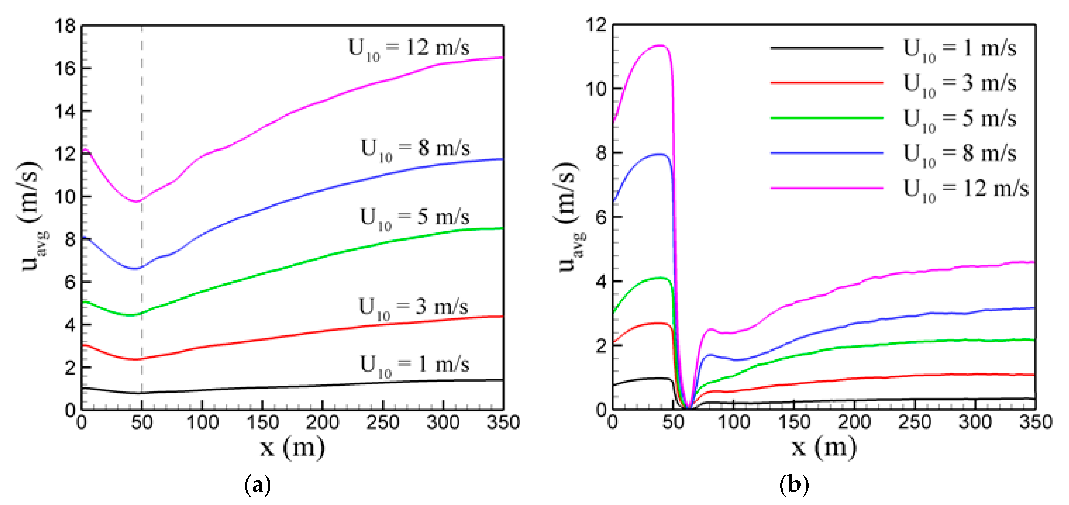
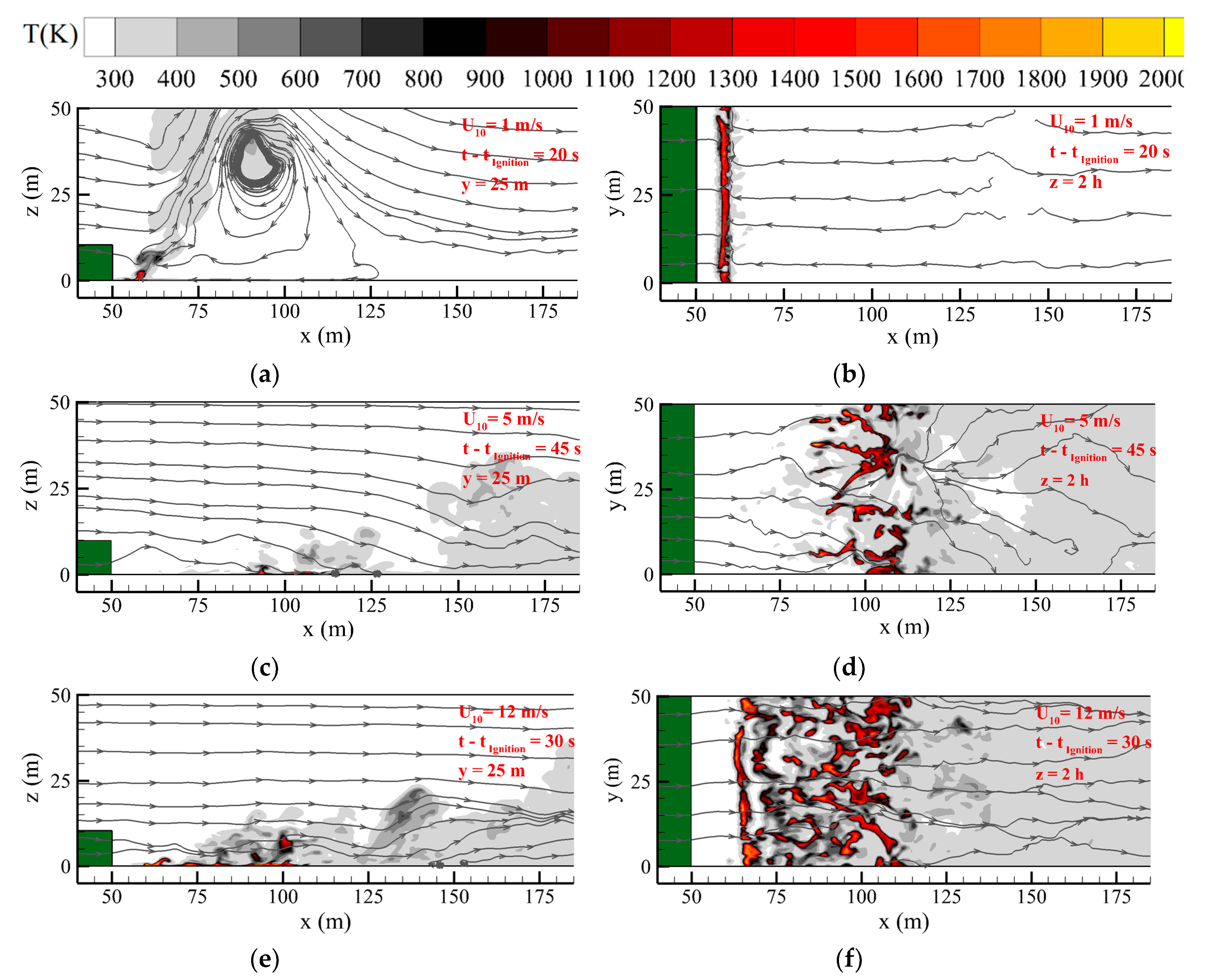
3.2.1. Flow Redevelopment

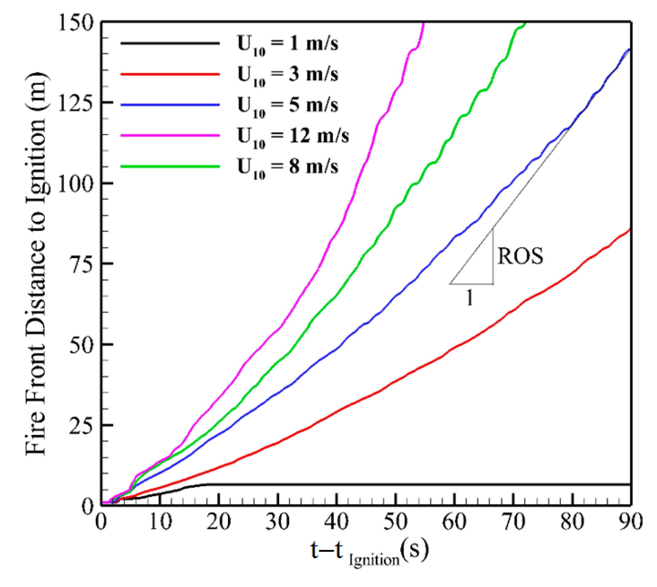
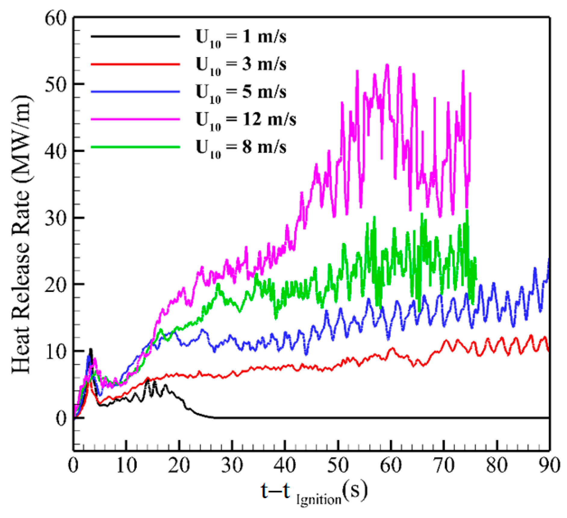
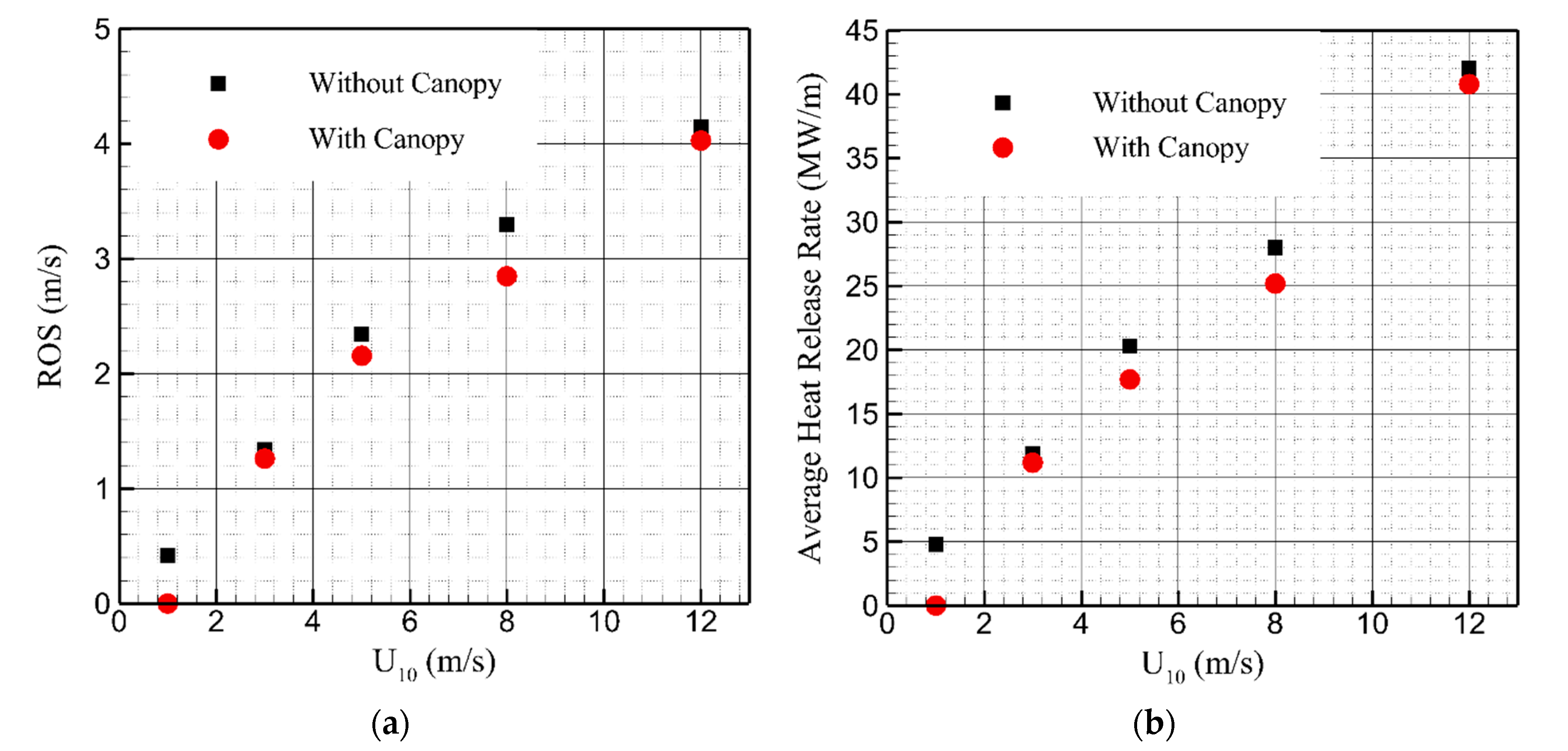
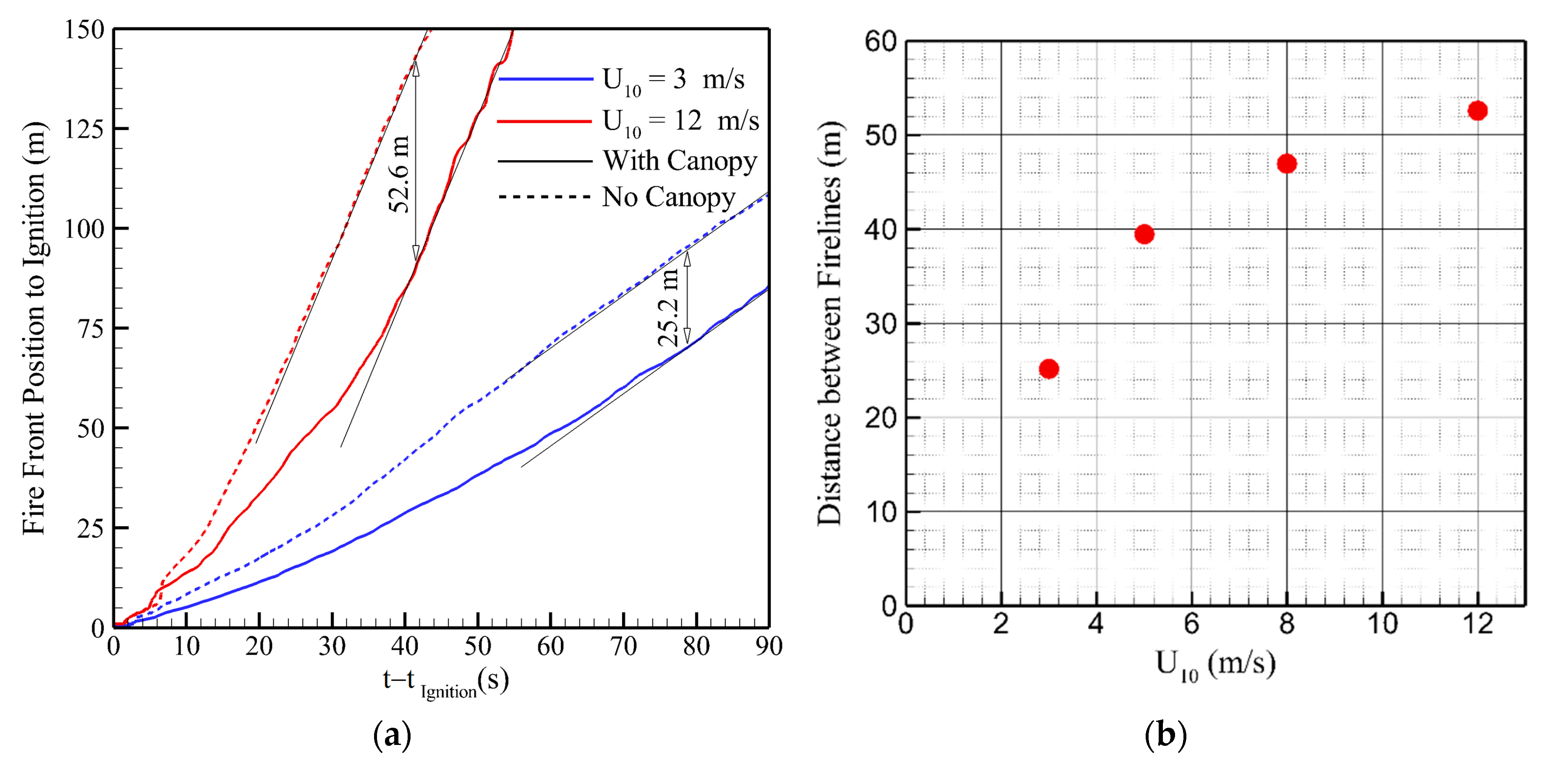
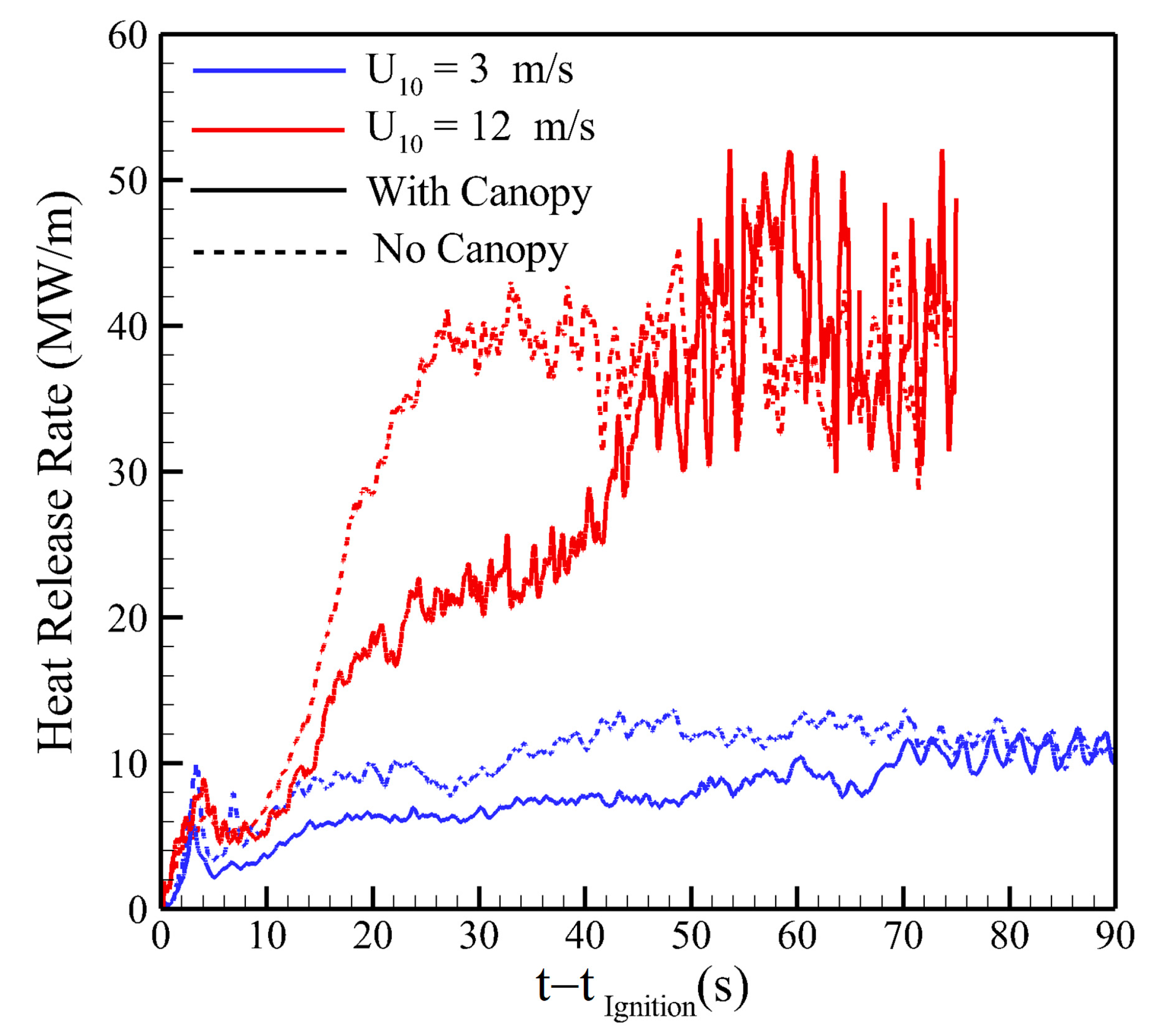
No persistent recirculation region was clearly observed downstream of the canopy for the average flow despite small transient regions of negative u-velocity as shown in the example flow in Figure 7. Sections at z = h through time-averaged flow fields, shown by Figure 8b, do not exhibit negative u-velocity values. There is a rapid decrease in velocity at x = 50 m and the u-velocity at x = 60 m is approximately zero in all cases, but the u-velocity rapidly increases at approximately x = 75 m. The transient regions of negative velocity in Figure 7 do not extend from the ground to the canopy top, and thus, we do not see recirculation regions as observed by Cassiani et al. [5], for example. The simulations of Cassiani et al. [5] with similar canopy density (LAI = 2) did not yield downstream of recirculation regions in agreement with our simulations. However, Cassiani et al. [5] found persistent recirculation regions in simulations with larger LAI values. The absence of a persistent recirculation zone downstream of the canopy can be explained by the fact that in our simulations the distribution of canopy LAD was not uniform along the vertical direction z (see Figure 2); therefore, the free space between the ground and the crown base (the Crown Base Height) promoted the development of a sub-canopy wind-jet near the ground (as shown in Figure 5), and this mechanism prevented the formation of a recirculation zone [49].

Figure 8 shows that the average-streamwise velocity does not reach a constant value 300 m downstream of the canopy for all wind speeds and therefore the redevelopment distance for the wind is greater than 300 m. An interesting feature of the 10 m high wind speeds is that the redeveloping wind speed exceeds the inlet wind speed in all cases. While no recirculation regions are observed, the fuel-height u-velocity immediately downstream of the canopy is approximately zero and is followed by a sharp rise between about x = 60 and 70 m (Figure 8b). Therefore, upon ignition, the fire will feel an initially very low driving velocity. This suggests that the rough-to-smooth transition (forest/grass transition) promotes an incoming flow from the upper boundary. This acceleration of the longitudinal flow near the ground in the clearing, noticed in the simulations and the downward incoming flow from the upper boundary, have also been clearly observed experimentally [50]. These two coupled phenomena are respectively due to the reduction of the drag force in the clearing and to the resulting mass conservation in the atmospheric boundary-layer.

3.2.2. Fire Spread

Fire-management analysts typically require estimates of quasi-equilibrium RoS and fire intensity. Because the wind field redevelops behind a tree canopy, it is reasonable to expect that the fire behavior behind a canopy will be dynamic and the fire should intensify downstream of the canopy. However, if the wind speed in the wake of the canopy grows very slowly, it is possible that the fire may equilibrate at some lower rate-of-spread and intensity than could be expected in open, i.e., no-canopy, conditions. Empirical models [3] use WRF to model the effect of the canopy on the rate-of-spread and intensity of the fire [51]. However, WRF are only applied within canopies. It may be necessary to extend WRF models to include regions in the canopy wake. This requires quantifying the fire rate-of-spread and the length of fire-canopy wake development region.

Fire propagation is often characterized by two distinct modes: the buoyancy-dominated (sometimes called plume) mode and the wind-driven (occasionally called the boundary-layer) mode. The mode of an individual fire is distinguished by the Byram convection number, $Nc$, a non-dimensional ratio of buoyancy and wind kinetic energy [21,52]. Wind-driven fires are characterized by small values of Nc, while large values are encountered in plume-dominated fires. According to the literature [53], the transition between the two regimes of propagation occurs for 2 < Nc < 10. In the buoyancy-dominated mode, the flame is largely vertical and the fire is thought to spread largely by radiative heating of the fuel. In the wind-driven mode, the flame is more horizontal and convective heating is thought to be the dominant mechanism of heat transfer. For an idealized line fire, these modes are easily distinguished from the streamlines of the flow around the flame. In the buoyancy-driven mode the flame will entrain fresh air from both sides of the flame so the streamlines of the flow will converge onto the flame from both sides. In contrast, because the flame is more horizontal in the wind-driven mode, the flame will only entrain fresh air from the upstream side and the streamlines will only converge onto the flame from upstream of the flame. An intermediate regime, where the fire is neither truly buoyancy- nor wind-dominated, also exists. It is unclear if the fire oscillates between the buoyancy- and wind-dominated modes or if the fire persists in the intermediate state. Fires in the intermediate regime will likely have an inclined frame but two-sided entrainment. For these fires, the values of Nc, computed following [21] using the quasi-steady intensity and RoS, are (to the nearest integer): 114, 41, 11, and 4, respectively, for the cases U₁₀ = 3, 5, 8, and 12 m/s with a canopy, and 139, 58, 14, and 5, respectively, for the cases without a canopy. The Nc was evaluated after the fire reached a quasi-equilibrium spread rate using averaged RoS and intensity.

Isosurfaces of soot value, representative of the flame for U₁₀ = 1 m/s and U₁₀ = 12 m/s are shown in Figure 9. The U₁₀ = 1 m/s case is likely buoyancy dominated with a characteristically vertical flame, whereas the U₁₀ = 12 m/s case is likely wind dominated with a horizontal and attached flame. Figure 10 shows streamlines in vertical median and xy (z = 2h) planes around the flame for three cases: U₁₀ = 1, 3, and 12 m/s. The U₁₀ = 1 m/s case shows the flame entraining fluid from both sides and the U₁₀ = 12 m/s case shows the flame entraining from only upstream, confirming that these cases are buoyancy and wind dominated, respectively, despite the low intermediate N_c values. The U₁₀ = 5 m/s is more complicated and can be considered as a hybrid between these two regimes. The flame appears be attached but there is a complicated flow structure in front of the flame. The streamlines in the horizontal plane suggest that the flow is predominantly from left to the right of the domain, even though there is a plume present. The entrainment of fresh air into the plume is therefore on the upstream side only. This suggests that this fire is a more wind-dominated fire than a buoyancy-dominated fire. The U₁₀ = 5 m/s case streamlines can be contrasted with those of the U₁₀ = 1 m/s case, which clearly shows entrainment on both sides of the flame. In the U₁₀ = 1 m/s case there is a large vortex structure generated by the plume; however, it is not a canopy-induced recirculation region as observed by Cassiani et al. [5]. Canopy induced recirculation regions occur directly behind the canopy and extend from the ground to the canopy top. The horizontal plane z = 2h images in Figure 10 also show differences in the flame structure. For the U₁₀ = 1 m/s case, the flame depth (the distance in the x-direction between the two edges of the burning region) is very small and the burning region is largely continuous in the spanwise directions. However, small interruptions to the flaming zone are present at the edges and center of the domain. Small vortex-pair structures can be seen at the edges of the individual flaming regions (e.g., at approximately (x,y) = (65,10) m). In the U₁₀ = 5 m/s case, the flame structure is considerably different: long streak-like structures are visible and the flame depth is approximately 25 m (at z = 2h). In the U₁₀ = 12 m/s case, the flame structure at z = 2h is patchier. The front is considerably deeper, approximately 50 m than the other two cases. Both of these observations are consistent with a more inclined and attached flame.

The fire-front location (relative to the ignition line) was determined by finding, at each time step, the average position of the most remote points at the grassland surface downstream the ignition line that are characterized by zero dry-material mass fraction (i.e., pyrolysis front at the grassland surface). An example contour diagram showing the fuel composition is presented in Figure 11. The front location (average of the pyrolysis front position in the y-direction at the grassland surface) is shown in Figure 12 as a function of time. The U₁₀ = 1 m/s case extinguishes at approximately 15 m downstream of the ignition location. The wind velocity at flame height is very low (see Figure 8b) and is likely insufficient to sustain a propagating fire in this particular fuel bed. All other cases propagate to the end of the domain in an approximately quasi-equilibrium manner, as indicated by the approximately-linear behavior of frontal location with time. All of the average-frontal positions as a function of time shown in Figure 12 are slightly nonlinear, indicating that the fires are slowly accelerating.

The fireline intensity, shown in Figure 13 per unit of fireline length (i.e., the domain width), was estimated from the total heat release rate (HRR) and the domain width. The HRR is given by Equation (2), where ω_vap, ω_pyr, ω_char, ω_CO, and ω_soot are, respectively, the total mass rates of water evaporation, pyrolysis, char combustion, combustion of CO in the gas mixture, and soot combustion, and ΔH_vap, ΔH_pyr, ΔH_char, ΔH_CO, and ΔH_soot are the corresponding specific heats. Note that ΔH_char is not constant; it depends on the proportion of CO to CO₂ produced during charcoal combustion [21], and it varies between 9 MJ/kg (for incomplete combustion) and 30 MJ/kg (for complete combustion).

$$HRR=-{\omega }_{vap}·\Delta H_{vap}-{\omega }_{pyr}·\Delta H_{pyr}+{\omega }_{char}·\Delta H_{char}+{\omega }_{CO}·\Delta H_{CO}+{\omega }_{soot}·\Delta H_{soot}$$

(2)

All fires follow roughly similar trends with a spike in intensity at ignition. The U₁₀ = 1 m/s case shows a brief period (between approximately 10 and 20 s) of quasi-equilibrium intensity, consistent with the period of linear growth in frontal location (Figure 12), before the intensity decays to zero as the fire extinguishes. The other cases grow towards a quasi-equilibrium intensity; however, with the exception of the U₁₀ = 12 m/s case, the intensity still grows very slowly throughout the simulation. The U₁₀ = 3, 5, and 8 m/s cases tend towards intensities of 8, 14, and 20 MW/m, respectively. The amplitude of the variance in intensity also increases with time. The U₁₀ = 12 m/s behaves differently; the intensity peaks at around 60 s before decaying and re-intensifying between 60–80 s. This is suggestive of surge-stall behavior [54], which is consistent with the step-like changes in the frontal location that emerge at approximately 50 s after ignition. The variation of the intensity also increases with wind speed across all cases. The U₁₀ = 10 m/s case also exhibits step-like behavior in the frontal location, and some regular bursting in the intensity occurs at 55, 65, and 75 s after ignition. However, further investigation is required to completely characterize the fire behavior over this regime.

The average quasi-equilibrium RoS was determined from the gradient of the most linear section of the fire location as a function of time [55]. The average RoS and intensities of the fires in open grassland (without the canopy) and downstream of the canopy are compared in Figure 14. Firstly, the open U₁₀ = 1 m/s case does not extinguish, suggesting that the sheltered wind speed downstream of the canopy is insufficient to sustain the fire when a canopy is present. The canopy does reduce the average RoS; however, the effect is minor. The largest difference of approximately 15% occurs in the U₁₀ = 8 m/s case (Figure 14a). The average intensity is also systematically lower downstream of a canopy than in the open by approximately 10% (Figure 14b). On the other hand, the average RoS and fire intensity obtained at steady state of fire spread are in agreement with experimental data [56] and with predictions of other numerical studies [18,57] and empirical models [3,58].

To quantify the implications of these differences, the average distances between fire fronts in the open and canopy cases are shown in Figure 15. To illustrate the differences, Figure 15a compares the frontal locations of the open (without canopy) and canopy cases with U₁₀ = 3 m/s and U₁₀ = 12 m/s. The fires in open grassland are significantly further, approximately 50 m for t > 30 s in the U₁₀ = 12 m/s case, ahead of the fires where a canopy is present. The distance systematically increases with wind speed, as shown in Figure 15b, although the rate of growth decreases with increasing wind speed. The U₁₀ = 12 m/s case frontal locations differ by 52 m. The intensity development shown in Figure 16 exhibits a similar delay. The U₁₀ = 3 m/s case recovers to the open intensity at approximately 70 s after ignition, and the U₁₀ = 12 m/s case recovers after approximately 50 s after ignition. The critical point between the two parts of the curve (sharp at the beginning and flatter at the end) seems to occur at U₁₀ = 8 m/s, which also corresponds to the beginning of the fully wind-driven regime for the fire propagating through the canopy free region. In fact, it is for this value of the wind speed that the Byram convective number reaches a value nearly equal to 11 (> 10 i.e., the beginning of the fully wind-driven fire regime). In analyzing the fire intensity history in Figure 13 and in considering the sudden increase of fluctuations highlighted for U₁₀ = 8 and 12 m/s, compared to the results obtained for lower values of the wind speed, we could conclude that for safety reasons, prescribed burning would be more suitable (in this configuration) for wind speed at least smaller than 5 m/s.

Because the fires downstream of a canopy recover to the open RoS and intensity after maximum of approximately 50 m, the use of modified fire-spread models in the wake of a canopy may be unnecessary. However, the recovery distance will likely depend on canopy height and LAI, which were constant throughout these simulations. Therefore, a more extensive parameter space investigation is required for some operationally useful criteria for fire redevelopment can be quantified. Interestingly, while the fire RoS and intensities largely recovered after 50 m downstream of, the fuel height u-velocity shown in Figure 8 requires about three times the distance to recover to an equilibrium value. Further investigation is required to understand the link between wind speed variation and fire behavior.

4. Conclusions

LES of grassland fires propagating downstream of a forest canopy were carried out to model a situation similar to that encountered in a fuel break or a clearing. To accurately reproduce the flow conditions observed on the field in such a situation, a two-phase approach was used in order to reproduce correctly, at the inlet of the computational domain, the turbulent flow resulting from the interaction between an ABL flow and a homogeneous canopy (reproducing a pine forest).

The first phase of the study (ABL/canopy turbulent flow with periodic lateral boundary conditions), correctly reproduced the pathway between the initial development of a quasi-twotwo-dimensional (2D) Kelvin-Helmholtz instability, characterized by the formation of spanwise vortices, to a fully three-dimensional (3D) fully-turbulent flow. The simulations showed that, provided that the calculations were performed during a sufficiently long time (about 1500 s), a statistically-stationary turbulent flow can be achieved. All the results obtained in this preliminary part were in agreement with the data published in the literature on this subject.

The second phase simulated fire propagation through a grassland, downstream of the canopy, which constituted the heart of this study. This phase started by a flow-redevelopment step that was carried out for about 1000 s to make sure that a fully-developed turbulent flow exists downstream of the canopy before fire ignition. The numerical results clearly showed that the range of the wind speed (from 1 to 12 m/s) covered both buoyancy-dominated and wind-driven fire regimes of propagation. For the smallest value of the wind speed (1 m/s), the sheltering effect due to the location of the ignition line near the forest prevented the propagation of the fire beyond 25 s. In all other cases, the fire was able to propagate without any interruption, which is the objective during a prescribed burning operation.

In these simulations, we did not find recirculation regions downstream of the canopy, because the canopy we considered was relatively sparse. We found that the fire width and flame structure changed with wind speed. At low wind speeds, we found narrower vertical flames, which would be expected for buoyancy-dominated fires, while at higher wind speeds, we found elongated flames with a streaky-structure characteristic of a wind-dominated fire. The rate of fire spread and heat release rate for fires downstream of a canopy were only slightly lower than for fires in open grassland (without a canopy). However, the presence of a canopy made significant differences to the overall fire development: the heat release rate takes significantly-longer time to reach the equilibrium value when a canopy is present, and the fire downstream of a canopy lagged the fire in open grassland by 50 m in the 12 m/s wind speed case.

The curves representing the time evolution of the fire intensity allowed to define some suitable conditions for the implementation of prescribed burning operations. These preliminary results demonstrated the interest of using this kind of physical fire model, even to study practical operational configurations, at least to highlight the global trend of some parameters. However, we cannot consider that we have fully understood the impact of even simple parameters, such as the wind, the slope, the fuel moisture content, or the coupling between these various physical parameters on the behavior of wildfires, especially in three dimensions. Therefore, a considerable amount of additional work is required to progress in the understanding of the fire behavior, in order to improvement fire-safety engineering.

References

1. The Guardian. Explainer: How Effective Is Bushfire Hazard Reduction on Australia’s Fires? Available online: https://www.theguardian.com/australia-news/2020/jan/05/explainer-how-effective-is-bushfire-hazard-reduction-on-australias-fires (accessed on 5 June 2020).
2. Moon, K.; Duff, T.J.; Tolhurst, K.G. Sub-canopy forest winds: Understanding wind profiles for fire behaviour simulation. Fire Saf. J. 2019, 105, 320–329. [Google Scholar] [CrossRef]
3. McArthur, A.G. Fire Behaviour in Eucalypt Forests; Leaflet No. 107; Forestry and Timber Bureau: Canberra, Australia, 1967. [Google Scholar]
4. Andrews, P.L. Modeling Wind Adjustment Factor and Midflame Wind Speed for Rothermel’s Surface Fire Spread Model; Contract N° RMRS-GTR-266; Rocky Mountain Research Station, Department of Agriculture/Forest Service: Fort Collins, CO, USA, 2012.
5. Cassiani, M.; Katul, G.G.; Albertson, J.D. The effects of canopy leaf area index on airflow across forest edges: Large-eddy simulation and analytical results. Bound. Layer Meteorol. 2008, 126, 433–460. [Google Scholar] [CrossRef] [Green Version]
6. Bohrer, G.; Katul, G.G.; Walko, R.L.; Avissar, R. Exploring the effects of microscale structural heterogeneity of forest canopies using large-eddy simulations. Bound. Layer Meteorol. 2009, 132, 351–382. [Google Scholar] [CrossRef]
7. Dupont, S.; Bonnefond, J.-M.; Irvine, M.R.; Lamaud, E.; Brunet, Y. Long-distance edge effects in a pine forest with a deep and sparse trunk space: In situ and numerical experiments. Agric. For. Meteorol. 2011, 151, 328–344. [Google Scholar] [CrossRef]
8. Dupont, S.; Irvine, M.; Bonnefond, J.-M.; Lamaud, E.; Brunet, Y. Turbulent structures in a pine forest with a deep and sparse trunk space: Stand and edge regions. Bound. Layer Meteorol. 2012, 143, 309–336. [Google Scholar] [CrossRef]
9. Belcher, S.E.; Harman, I.N.; Finnigan, J.J. The wind in the willows: Flows in forest canopies in complex terrain. Annu. Rev. Fluid Mech. 2012, 44, 479–504. [Google Scholar] [CrossRef]
10. Schlegel, F.; Stiller, J.; Bienert, A.; Maas, H.G.; Queck, R.; Bernhofer, C. Large-eddy simulation study of the effects on flow of a heterogeneous forest at sub-tree resolution. Bound. Layer Meteorol. 2015, 154, 27–56. [Google Scholar] [CrossRef]
11. Sutherland, D.; Philip, J.; Ooi, A.; Moinuddin, K. Simulations of surface fire propagating under a canopy: Flame angle and intermittency. In Proceedings of the 8th ICFFR, Advances in Forest Fire Research 2018, Coimbra, Portugal, 9–16 November 2018; Viegas, D.X., Ed.; Imprensa da Universidade de Coimbra: Coimbra, Portugal, 2018; pp. 1303–1307. [Google Scholar] [CrossRef] [Green Version]
12. Morvan, D.; Dupuy, J.L. Modeling the propagation of a wildfire through a Mediterranean shrub using a multiphase formulation. Combust. Flame 2004, 138, 199–210. [Google Scholar] [CrossRef]
13. Frangieh, N.; Morvan, D.; Meradji, S.; Accary, G.; Bessonov, O. Numerical simulation of grassland fires behavior using an implicit physical multiphase model. Fire Saf. J. 2018, 102, 37–47. [Google Scholar] [CrossRef] [Green Version]
14. Gavrilov, K.; Morvan, D.; Accary, G.; Lyubimov, D.; Meradji, S. Numerical simulation of coherent turbulent structures and of passive scalar dispersion in a canopy sub-layer. Comput. Fluids 2013, 78, 54–62. [Google Scholar] [CrossRef]
15. Gavrilov, K.; Accary, G.; Morvan, D.; Dmitry, L.; Meradji, S.; Bessonov, O. Numerical simulation of coherent structures over plant canopy. Flow Turb. Comb. 2011, 86, 89–111. [Google Scholar] [CrossRef]
16. Nepf, H.; Ghisalberti, M.; White, B.; Murphy, E. Retention time and dispersion associated with submerged aquatic canopies. Water Resour. Res. 2007, 43, 4. [Google Scholar] [CrossRef]
17. Hu, X.; Lee, X.; Stevens, D.E.; Smith, R.B. A numerical study of nocturnal wavelike motion in forests. Bound. Meteorol. 2002, 102, 199–223. [Google Scholar] [CrossRef]
18. Frangieh, N.; Accary, G.; Morvan, D.; Meradji, S.; Bessonov, O. Wildfires front dynamics: 3D structures and intensity at small and large scales. Combust. Flame 2020, 211, 54–67. [Google Scholar] [CrossRef]
19. Frangieh, N.; Morvan, D.; Accary, G.; Meradji, S. Front’s dynamics of quasi-infinite grassland fires. In Proceedings of the 8th ICFFR, Advances in Forest Fire Research 2018, Coimbra, Portugal, 9–16 November 2018; Viegas, D.X., Ed.; Imprensa da Universidade de Coimbra: Coimbra, Portugal, 2018; pp. 1024–1034. [Google Scholar] [CrossRef]
20. Morvan, D.; Meradji, S.; Accary, G. Physical modelling of fire spread in Grasslands. Fire Saf. J. 2009, 44, 50–61. [Google Scholar] [CrossRef]
21. Morvan, D.; Accary, G.; Meradji, S.; Frangieh, N.; Bessonov, O. A 3D physical model to study the behavior of vegetation fires at laboratory scale. Fire Saf. J. 2018, 101, 39–52. [Google Scholar] [CrossRef] [Green Version]
22. Grishin, A.M. Mathematical Modeling of Forest Fires and New Methods for Fighting Them; Albini, F., Ed.; Publishing House of the Tomsk University: Tomsk, Russia, 1997. [Google Scholar]
23. Morvan, D.; Dupuy, J.L. Modeling of fire spread through a forest fuel bed using a multiphase formulation. Combust. Flame 2001, 127, 1981–1994. [Google Scholar] [CrossRef]
24. Morvan, D.; Meradji, S.; Accary, G. Wildfire behavior study in a Mediterranean pine stand using a physically based model. Combust. Sci. Technol. 2008, 180, 230–248. [Google Scholar] [CrossRef]
25. Favre, A.; Kovasznay, L.S.G.; Dumas, R.; Gaviglio, J.; Coantic, M. La Turbulence en Mécanique des Fluides; Gauthier-Villars: Paris, France, 1976. [Google Scholar]
26. Cox, G. Combustion Fundamentals of Fire; Academic Press: Cambridge, MA, USA, 1995. [Google Scholar]
27. Gavrilov, K. Numerical Modeling of Atmospheric Flow over Forest Canopy. Ph.D. Thesis, Aix-Marseille University, Marseille, France, 2001. [Google Scholar]
28. Kee, R.J.; Rupley, F.M.; Miller, J.A. The Chemkin Thermodynamic Data Base; Technical Report SAND87-8215B; Sandia National Laboratories: Albuquerque, NM, USA, 1990. [Google Scholar]
29. Magnussen, B.F.; Mjertager, B.H. On mathematical modeling of turbulent combustion. Combust. Sci. Technol. 1998, 140, 93–122. [Google Scholar]
30. Syed, K.J.; Stewart, C.D.; Moss, J.B. Modelling soot formation and thermal radiation in buoyant turbulent diffusion flames. Symp. (Int.) Combust. 1991, 23, 1533–1541. [Google Scholar] [CrossRef]
31. Moss, J.B. Turbulent diffusion flames. In Forest Fire Control and Use; Cox, G., Ed.; Academic Press: London, UK, 1990. [Google Scholar]
32. Nagle, J.; Strickland-Constable, R.F. Oxidation of carbon between 1000–2000 °C. In Proceedings of the 5th Conference on Carbon, State College, PA, USA, 19–23 June 1961; Pergamon Press: Oxford, UK, 1962; pp. 154–164. [Google Scholar] [CrossRef]
33. Incropera, F.P.; DeWitt, D.P. Fundamentals of Heat and Mass Transfer; John Wiley and Sons: Hoboken, NJ, USA, 1996. [Google Scholar]
34. Siegel, R.; Howell, J.R. Thermal Radiation Heat Transfer, 3rd ed.; Hemisphere Publishing Corporation: Washington, DC, USA, 1992. [Google Scholar]
35. Patankar, S.V. Numerical Heat Transfer and Fluid Flow; Hemisphere Publishing: New York, NY, USA, 1980. [Google Scholar]
36. Versteeg, H.K.; Malalasekera, W. An Introduction to Computational Fluid Dynamics, the Finite Volume Method; Prentice Hall: Upper Saddle River, NJ, USA, 2007. [Google Scholar]
37. Li, Y.; Rudman, M. Assessment of higher-order upwind schemes incorporating FCT for convection-dominated problems. Numer. Heat Transf. Part B Fundam. 1995, 27, 1–21. [Google Scholar] [CrossRef]
38. Ferziger, J.H.; Peric, M.; Leonard, A. Computational Methods for Fluid Dynamics; Springer: New York, NY, USA, 2002. [Google Scholar] [CrossRef]
39. Modest, M.F. Radiative Heat Transfer; Academic Press: Cambridge, MA, USA, 2003. [Google Scholar]
40. Kaplan, C.R.; Baek, S.W.; Oran, E.S.; Ellzey, J.L. Dynamics of a strongly radiating unsteady ethylene jet diffusion flame. Combust. Flame 1994, 96, 1–21. [Google Scholar] [CrossRef]
41. Accary, G.; Bessonov, O.; Fougere, D.; Meradji, S.; Morvan, D. Optimized parallel approach for 3D modelling of forest fires behaviour. In LNCS; Malyshkin, V., Ed.; Parallel Computing Technologies; Springer: Berlin/Heidelberg, Germany, 2007; Volume 4671, pp. 96–102. [Google Scholar] [CrossRef]
42. Accary, G.; Bessonov, O.; Fougere, D.; Gavrilov, K.; Meradji, S.; Morvan, D. Efficient parallelization of the preconditioned conjugate gradient method. In LNCS; Malyshkin, V., Ed.; Parallel Computing Technologies; Springer: Berlin/Heidelberg, Germany, 2009; Volume 5968, pp. 60–72. [Google Scholar] [CrossRef]
43. Bessonov, O.; Meradji, S. Efficient Parallel Solvers for the FireStar3D Wildfire Numerical Simulation Model. In LNCS; Malyshkin, V., Ed.; Parallel Computing Technologies; Springer: Berlin/Heidelberg, Germany, 2019; Volume 11657, pp. 140–150. [Google Scholar] [CrossRef]
44. Khalifah, A.; Accary, G.; Meradji, S.; Scarella, G.; Morvan, D.; Kahine, K. Three-dimensional numerical simulation of the interaction between natural convection and radiation in a differentially heated cavity in the low Mach number approximation using the discrete ordinates method. In Proceedings of the 4th Int. Conf. on Thermal Engineering: Theory and Application, Abu Dhabi, UAE, 12–14 January 2009. [Google Scholar]
45. Accary, G.; Meradji, S.; Fougere, D.; Morvan, D. Towards a numerical benchmark for 3D mixed-convection low Mach number flows in a rectangular channel heated from below. J. Fluid Dyn. Mater. Sci. 2008, 141, 1–7. [Google Scholar]
46. Finnigan, J. Turbulence in plant canopies. Annu. Rev. Fluid Mech. 2000, 32, 519–571. [Google Scholar] [CrossRef]
47. Hunt, J.C.; Wray, A.A.; Moin, P. Eddies, streams, and convergence zones in turbulent flows. In Proceedings of the Summer Program 1988; Center for Turbulence Research: Stanford, CA, USA, 1988; pp. 193–208. [Google Scholar]
48. Amiro, B.D. Drag coefficients and turbulence spectra within three boreal forest canopies. Bound. Layer Meteorol. 1990, 52, 227–246. [Google Scholar] [CrossRef]
49. Dupont, S.; Brunet, Y. Edge flow and canopy structure: A large-eddy simulation study. Bound. Layer Meteorol. 2008, 126, 51–71. [Google Scholar] [CrossRef]
50. Raupach, M.R.; Bradley, E.F.; Ghadiri, H. A Wind Tunnel Investigation into the Aerodynamics Effect of Clearings on the Nesting of Abbott’s Boody on Christmas Island; Internal Report; CSIRO, Centre for Environmental Mechanics: Canberra, Australia, 1987. [Google Scholar]
51. Massman, W.J.; Forthofer, J.M.; Finney, M.A. An improved canopy wind model for predicting wind adjustment factors and wildland fire behavior. Canad. J. For. Res. 2017, 47, 594–603. [Google Scholar] [CrossRef] [Green Version]
52. Byram, G.M. Combustion of forest fuels. In Forest Fire: Control and Use; Davis, K.P., Ed.; McGraw Hill: New York, NY, USA, 1959; pp. 61–89. [Google Scholar]
53. Morvan, D.; Frangieh, N. Wildland fires behaviour: Wind effect versus Byram’s convective number and consequences upon the regime of propagation. Int. J. Wildland Fire 2018, 27, 636–641. [Google Scholar] [CrossRef]
54. Dold, J.W.; Zinoviev, A. Fire eruption through intensity and spread rate interaction mediated by flow attachment. Combust. Theor. Model. 2009, 13, 763–793. [Google Scholar] [CrossRef]
55. Moinuddin, K.A.M.; Sutherland, D.; Mell, W. Simulation study of grass fire using a physics-based model: Striving towards numerical rigour and the effect of grass height on the rate of spread. Int. J. Wildland Fire 2018, 27, 800–814. [Google Scholar] [CrossRef]
56. Cheney, N.P.; Gould, J.S.; Catchpole, W.R. Prediction of fire spread in grasslands. Int. J. Wildland Fire 1998, 8, 1–13. [Google Scholar] [CrossRef]
57. Linn, R.R.; Cunningham, P. Numerical simulations of grass fires using a coupled atmosphere-fire model: Basic fire behavior and dependence on wind speed. J. Geophys. Res. Atmos. 2005, 110, 110. [Google Scholar] [CrossRef]
58. Rothermel, R.C. A Mathematical Model for Predicting Fire Spread in Wildland Fuels; Research Paper INT-115; USDA Forest Service: Washington, DC, USA, 1972.
Figure 1. Two-dimensional (2D) view of the computational domain and boundary conditions used for phase 1. Domain width was 50 m in the y-direction with periodic boundary conditions.
Atmosphere 11 00683 g001
Figure 2. Distribution of the canopy leaf-area-density (LAD) in the vertical z-direction obtained from Equation (1), corresponding to a leaf-area-index (LAI) = 0.5, 2, and 8.
Atmosphere 11 00683 g002
Figure 3. 2D view of the computational domain and boundary conditions used for phase 2. Domain width is 50 m in the y-direction with periodic boundary conditions.
Atmosphere 11 00683 g003
Figure 4. Iso-surface Q = 2 s−2 of the Q-criterion, colored by the vertical velocity component, obtained in phase 1 for U10 = 5m/s and LAI = 2. (a) t = 15 s, (b) t = 20 s, (c) t = 1500 s (steady state).
Atmosphere 11 00683 g004
Figure 5. Effect of the wind speed (a) and the canopy LAI (b) on the normalized velocity profile u(z) (averaged in the x and the y directions and in time between t = 1200 s and t = 1500 s) obtained at steady state.
Atmosphere 11 00683 g005
Figure 6. Time evolution of stream-wise velocity component u obtained at steady state (t = 1300 s) at point (x = 100 m, z = H) for LAI = 2 and for U10 = 1 m/s (a) and 12 m/s (b).
Atmosphere 11 00683 g006
Figure 7. Vertical cross section of the stream-wise velocity field obtained at t = 1000 s, for canopy LAI = 2 and U10 = 5 m/s, at y = 25 m.
Atmosphere 11 00683 g007
Figure 8. Variation in the x-direction of the averaged stream-wise velocity component u obtained (a) at the canopy-top surface (z = H) and (b) at the grassland-top surface (z = h), for canopy LAI = 2 and for different wind speeds. u(x) was time-averaged between t = 800 s and t = 1000 s as well as in the y-direction.
Atmosphere 11 00683 g008
Figure 9. Three-dimensional (3D) views of grassland fire spread downstream of a canopy obtained for U10 = 1 m/s (a) and U10 = 12 m/s (b), 20 s and 30 s, respectively, after ignition. Fire is visualized by an isovalue surface of the soot volume fraction (10−6) colored by the gas temperature and by an isovalue surface of the water mass-fraction (0.00075) in grey shades with 75% transparency.
Atmosphere 11 00683 g009
Figure 10. Cuts in the vertical-median plane y = 25 m (a,c,e) and in the horizontal plan z = 2h (b,d,f) of the temperature field with streamlines obtained for U10 = 1 m/s (a,b), 5 m/s (c,d), and 12 m/s (e,f).
Atmosphere 11 00683 g010
Figure 11. Distribution of the fuel composition at the grassland surface (z = h), obtained 45 s after ignition (tIgnition = 1000 s in phase 2) in the case of U10 = 5 m/s, showing the position of the fire front.
Atmosphere 11 00683 g011
Figure 12. Time evolution of the average position of the fire front at the grassland surface obtained for different wind speeds. The rate of spread (RoS) is the slope of the curve at steady fire propagation.
Atmosphere 11 00683 g012
Figure 13. Time evolution the total heat release rate per unit length of fire line obtained for different wind speeds from Equation (2).
Atmosphere 11 00683 g013
Figure 14. (a) Rates of fire spread obtained at steady state for different wind speeds in the presence of a canopy compared to those obtained for the same simulation conditions but without a canopy. (b) Average heat release rates obtained at steady state for different wind speeds in the presence of a canopy compared to those obtained for the same simulation conditions but without a canopy.
Atmosphere 11 00683 g014
Figure 15. (a) Time evolution of the average position of the fire front at the grassland surface obtained for U10 = 3 m/s and 12 m/s in the case of fire spread downstream of a canopy, compared to the case of fire spread obtained for the same simulation conditions but without a canopy. (b) Distance between the fire position obtained at steady state with and without the presence of a canopy upstream the grassland for all cases except the U10 = 1 m/s case.
Atmosphere 11 00683 g015
Figure 16. Time evolution of the heat release rate obtained from Equation (2) for U10 = 3 m/s and 12 m/s in the case of fire spread downstream of a canopy, compared to the case of fire spread obtained for the same simulation conditions but without a canopy.
Atmosphere 11 00683 g016