Seasonal Variations of High-Frequency Gravity Wave Momentum Fluxes and Their Forcing toward Zonal Winds in the Mesosphere and Lower Thermosphere over Langfang, China (39.4° N, 116.7° E)

Abstract

Meteor radar data collected over Langfang, China (39.4° N, 116.7° E) were used to estimate the momentum flux of short-period (less than 2 h) gravity waves (GWs) in the mesosphere and lower thermosphere (MLT), using the Hocking (2005) analysis technique. Seasonal variations in GW momentum flux exhibited annual oscillation (AO), semiannual oscillation (SAO), and quasi-4-month oscillation. Quantitative estimations of GW forcing toward the mean zonal flow were provided using the determined GW momentum flux. The mean flow acceleration estimated from the divergence of this flux was compared with the observed acceleration of zonal winds displaying SAO and quasi-4-month oscillations. These comparisons were used to analyze the contribution of zonal momentum fluxes of SAO and quasi-4-month oscillations to zonal winds. The estimated acceleration from high-frequency GWs was in the same direction as the observed acceleration of zonal winds for quasi-4-month oscillation winds, with GWs contributing more than 69%. The estimated acceleration due to Coriolis forces to the zonal wind was studied; the findings were opposite to the estimated acceleration of high-frequency GWs for quasi-4-month oscillation winds. The significance of this study lies in estimating and quantifying the contribution of the GW momentum fluxes to zonal winds with quasi-4-month periods over mid-latitude regions for the first time.

1. Introduction

It is generally accepted that mid- and upper-atmosphere gravity waves (GWs) are generated primarily in the lower atmosphere [1]. During the upward transmission process, the energy and flux carried by GWs can be deposited into the mean flow of the mesosphere and lower thermosphere (MLT) region, thereby modulating MLT atmospheric circulation [2]. Fritts and Vincent proposed that high-frequency GWs with high intrinsic frequencies and small horizontal scales play a critical role in the transmission of momentum to the middle atmosphere [3]. This study investigates high-frequency atmospheric GWs in the MLT region, with periods of less than 2 h.

GWs can transmit and deposit momentum and energy from the lower to the upper atmosphere. The vertical flux of horizontal momentum (momentum flux) can be used to quantify this transfer and several observational studies have been conducted to estimate this momentum flux at a single site and globally. Satellites can be used to indirectly estimate global GW momentum flux using measured temperature profiles [4]. Ground-based observation techniques, such as medium frequency radar [5], airglow imaging [6,7], laser radar [8,9], and meteor radar [10,11,12,13,14,15,16,17,18,19,20,21] have been used to estimate GW momentum flux at single sites. Airglow imagers measure the momentum flux of a single GW event, rather than the average of many waves. Hocking extended the dual beam method to the meteor radar to measure GW momentum flux [10]. Meteor radar, used for all-weather observations, is relatively inexpensive, simple to install, and offers a wide deployment range. Thus, meteor radar is widely used to study GW momentum flux.

Existing studies show that there is a significant seasonal variation in GW momentum flux. There are annual oscillations (AOs) in GW momentum flux [15,19,20,21]. Several authors have used wind filtering theory to explain the phenomenon of AO in GW momentum flux [13,17]. GW momentum flux also exhibits semiannual oscillations (SAOs) [19,21]. Andrioli et al. first found a quasi-4-month oscillation in the zonal momentum flux of Santa Maria (30° S, 54° W) and the meridional momentum flux of Cachoeira Paulista (23° S, 45° W) at 92.5 km [15]. Pramitha et al. pointed out that the meridional momentum flux at the Tirupati (13.63° N, 79.4° E) station exhibited a quasi-4-month oscillation below 90 km [21].

GWs in lower layers have a significant influence on the structure and circulation of the MLT region [14]. GWs can dissipate in the middle layers and divergence from the resulting momentum flux can produce forces that accelerate mean atmospheric flow. Such forces drive a meridional circulation from the summer to winter pole at the solstices in the mid- and high-latitudes. Zonal momentum flux has specifically been investigated in previous studies to better understand this type of circulation. The relationship between the force generated by zonal momentum flux deposition and zonal wind has been demonstrated. de Wit et al. studied the relationship between the quasi-biennial oscillation modulation in GW momentum flux and the stratospheric quasi-biennial oscillation, which is consistent with the coupling of quasi-biennial oscillation modulation of the winter stratospheric vortex (through the Holton-Tan effect) to the summer mesopause through interhemispheric coupling [22]. de Wit et al. observed the annual variation in the relationship between the force of GW zonal momentum flux and zonal wind, which could be interpreted in terms of selective filtering of a uniform spectrum of vertically propagating GWs between the surface and mesopause region [17]. Antonita et al. found that SAO zonal wind was correlated with the force caused by GW momentum fluxes of SAO, and the contribution of high-frequency GWs was 20–70% [11]. Quasi-4-month oscillations were observed in GW momentum flux in low- and mid-latitudes, and Chen and Iimura et al. confirmed that there was also a quasi-4-month oscillation in the zonal wind [23,24]. However, it remains uncertain whether there is a potential relationship between a quasi-4-month oscillation in GW momentum flux and a quasi-4-month oscillation zonal wind.

The Langfang station is located in the mid-latitudes of the Eastern Hemisphere, and its meteor radar data can be used to study the characteristics of GW momentum flux and its effect on circulation, in order to understand whether the quasi-4-month oscillation zonal wind in the mid- and low-latitudes is related to GW, and to enrich our knowledge in this field. In this study, the seasonal variation characteristics of GW momentum flux and its effect on mean flow are studied using Langfang meteor radar data, in an attempt to understand the contribution of high-frequency GWs to the acceleration of SAO and quasi-4-month oscillation zonal wind in mid-latitude areas.

The remainder of this paper is organized as follows. Section 2 describes the meteor radar instrument, data set, and analysis methodology. Section 3 presents evidence for seasonal variations in GW momentum flux, observations and estimations of SAO and quasi-4-month mean flow acceleration. These results are discussed in Section 4 and Section 5 provides concluding remarks.

2. Data and Analysis Method

Meteor radar is an all-sky interferometric system that uses Doppler shifts in a coherent signal to effectively detect the radial velocities and positions of meteor trails within an altitude range of 70 to 110 km. From the measured radial velocity, zenith angle, azimuth angle, altitude, and detection time of the meteor trail, the atmospheric horizontal wind fields can be inverted and GW momentum flux can be calculated in the MLT region.

The meteor radar system at Langfang, China (39.4° N, 116.7° E) was established in July 2010. It offers a frequency of 35 MHz, maximum power of 20 kW, pulse width of 7.2 km, and pulse repetition frequency of 440 Hz. Data used in this study were acquired from 1 July 2010 to 31 July 2011 and were relatively continuous and complete over an altitude range of 80–101 km, which can be used for preliminary analysis of seasonal variations.

2.1. Momentum Flux Determination

Data analysis in this study was based on a technique developed by Hocking [10]. A composite day methodology was used to determine the GW momentum flux from the Langfang meteor radar measurements, with a specific focus on high-frequency waves with short periods (less than 2 h). These composite day measurements were accumulated from meteor trails, acquired over the course of a month, and consolidated into specific time/height bins representing single days. The data were then processed as though they had been acquired in one day [14,25,26]. The corresponding calculations are described below.

To study GWs with a period of less than 2 h, we chose 2-h time bins with a step size of 1 h and 3-km height bins. Altitude bins were established at 80–83, 83–86, 86–89, 89–92, 92–95, 95–98, and 98–101 km, with representative heights established at the midpoint of these altitude bins. Time bins were formed with a 2-h span in 1-h increments, up to 22:00–00:00 (i.e., 23:00–01:00, 00:00–02:00, etc.). The representative time was positioned at the midpoint of each bin.

Quality-control pre-processing was applied, as meteors located at smaller zenith angles typically produce larger horizontal velocity calculation errors, while meteors located at larger zenith angles often cause larger height measurement errors. As such, only meteor trails with zenith angles between 15° and 60° were included in the study [20]. In addition, meteors with radial velocities of more than 200 m/s often contain rapidly decaying fragments and were therefore discarded [13]. The number of meteors in each bin was not less than 10 to ensure the accuracy of background velocity field estimation [10,27,28]. The mean background wind (zonal, meridional, and vertical) was then calculated within each time/height bin for each day, using a least squares method. Meteor trails with a difference of more than 25 m/s between the actual radial velocity and the projected mean radial velocity were also excluded for quality-control purposes, and the least squares was repeated until there were no further meteor echoes excluded [27].

The exact height and time of meteors within each time/height bin were used to obtain a linearly interpolated mean wind at specific heights and times on each day, based on neighboring background winds (above, below, prior to, and after the current height-time box), as discussed in Liu et al. [14]. Values detected outside the background wind altitude range of 81.5 to 99.5 km were discarded during interpolation. New altitude bins were then formed for the interpolated mean wind, following GW analysis statistics, at 81.5–84.5, 84.5–87.5, …, and 96.5–99.5 km (centered at 83, 86, …, and 98 km).

Corresponding projected mean radial velocities were then calculated for each detected meteor using the interpolated mean wind. The perturbed radial velocity was then acquired by subtracting the corresponding projected mean radial velocity from the measured radial velocity of each detected meteor. Assuming the perturbed radial velocity obeyed a Gaussian distribution, the 5-standard-deviations criterion was used to remove outliers that were large enough to substantially bias the resulting momentum flux estimates [29].

Subsequent radial velocity perturbations were classified as composite day measurements for the corresponding month in 3-km height bins (centered at 83, 86, 89, 92, 95, and 98 km) and 2-h time bins with a step size of 1 h. The number of meteors in each time/height bin was not less than 30 to ensure the accuracy of calculating the momentum flux. Finally, the momentum fluxes were calculated according to the matrix as detailed by Hocking [10].

We can infer the following based on the discussion above: (1) For zonal and the meridional wind, each day was divided into 24-time bins and seven height bins, representing altitudes of 81.5, 84.5, 87.5, 90.5, 93.5, 96.5, and 99.5 km. A total of 168 time/height bins were established, each with a corresponding horizontal background wind field. (2) Zonal and meridional background wind and momentum flux were acquired for each time/height bin for composite days in each calendar month. The background wind data were then divided into 24-time bins and seven height bins (representing heights of 81.5, 84.5, 87.5, 90.5, 93.5, 96.5, and 99.5 km). The momentum flux data were divided into 24-time bins and six height bins (representing heights of 83, 86, 89, 92, 95, and 98 km), because values detected outside the background wind altitude range of 81.5 to 99.5 km were discarded during interpolation and the altitude bins were reclassified. The monthly mean background wind and momentum flux were then acquired by averaging different time bins within the same height range on the same composite day, in order to analyze seasonal variations in each parameter.

2.2. Estimation of Mean Flow Acceleration

Considering the equation of motion that represents the conservation of momentum, mass, and energy [30] in a Cartesian coordinate system, Eulerian mean equations can be expressed as:

$$\frac{\mathrm{d}\overline{\mathrm{u}}}{\mathrm{dt}}-\mathrm{f}\overline{v}=A$$

(1)

where $\overline{\mathrm{u}}$ represents zonal wind of zonal average and $\overline{v}$ represents meridional wind of zonal average. $A$ includes the acceleration due to the acting forces of GWs, planetary waves, tidal waves, and frictional and diabatic effects [31]. The term $\mathrm{f}\overline{v}$ represents the acceleration due to Coriolis forces, $\mathrm{f}=2\mathsf{\Omega }\sin \mathsf{\phi }$ is a Coriolis parameter, Ω is the rotational angular velocity of the earth, and $\mathsf{\phi }$ is the latitude.

The formula for calculating the acceleration of zonal wind caused by the divergence of GW momentum flux is as follows [3]:

$$\mathrm{X}=-\frac{1}{\rho }\frac{\partial \rho F_x}{\partial z}=\frac{F_x}{H}-\frac{\partial F_x}{\partial z}$$

(2)

where $\mathrm{X}$ is the corresponding acceleration, $F_x=\overline{u^{\prime }{w}^{\prime }}$ is the zonal momentum flux that varies with the height $z$, and the overbar represents an ensemble average. The first-order forward difference approximation was adopted in this study, which is defined as:

$$\frac{\partial F_x}{\partial \mathrm{z}}{│}_{z_i}=\frac{F_x\left(z_{i+1}\right)-F_x\left(z_i\right)}{z_{i+1}-z_i}$$

(3)

Here, H denotes the scale height given by:

$$H=\frac{RT}{g}$$

(4)

where T is the temperature, R is a gas constant (287 J/(kg*K)), and g denotes the gravitational acceleration determined using a formula published by the World Meteorological Organization in 1983:

$$\mathrm{g}=9.80616(1-0.002637\cos 2\mathsf{\phi }+0.0000059{\cos }^{2}2\mathsf{\phi })$$

(5)

In addition, based on the harmonic analysis of GW momentum flux and background wind for 12 months at each height using Fourier transformation, the amplitude and phase of the cosine function of SAO and quasi-4-month oscillation zonal momentum flux and background wind can be obtained, as can the time series of SAO and quasi-4-month oscillation.

By using Formula (2), we obtained the estimated acceleration of zonal wind produced by the momentum flux of the SAO and quasi-4-month oscillation. Assuming that the monthly average wind at the station is equal to the monthly zonal average wind, the semiannual and quasi-4-month oscillation components of the meridional wind were obtained by harmonic fitting, and the estimated acceleration caused by the Coriolis force was obtained. The observed acceleration of zonal wind can be estimated directly using the fitted cosine function. The above-estimated zonal wind acceleration, Coriolis force, and high-frequency GW force can be used to analyze and discuss the contribution of GW to the mean flow.

3. Observations and Results

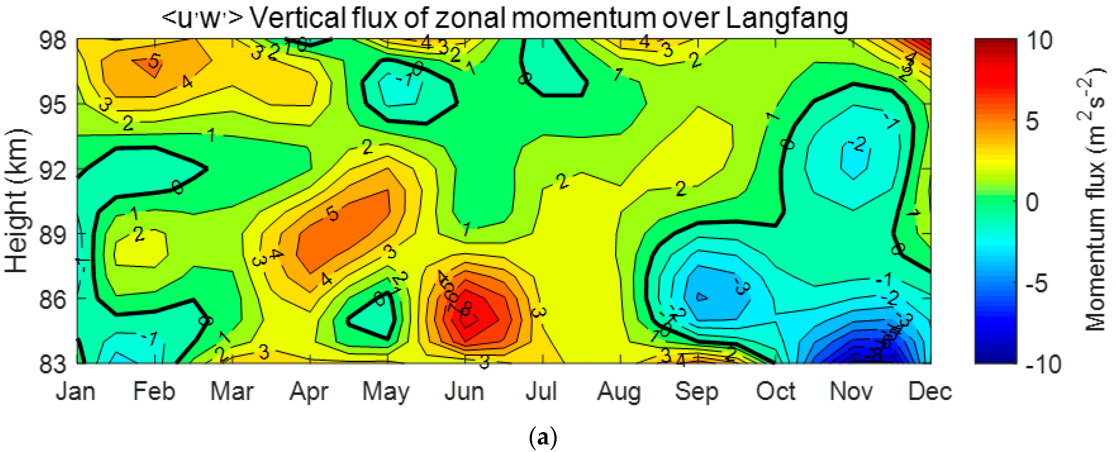
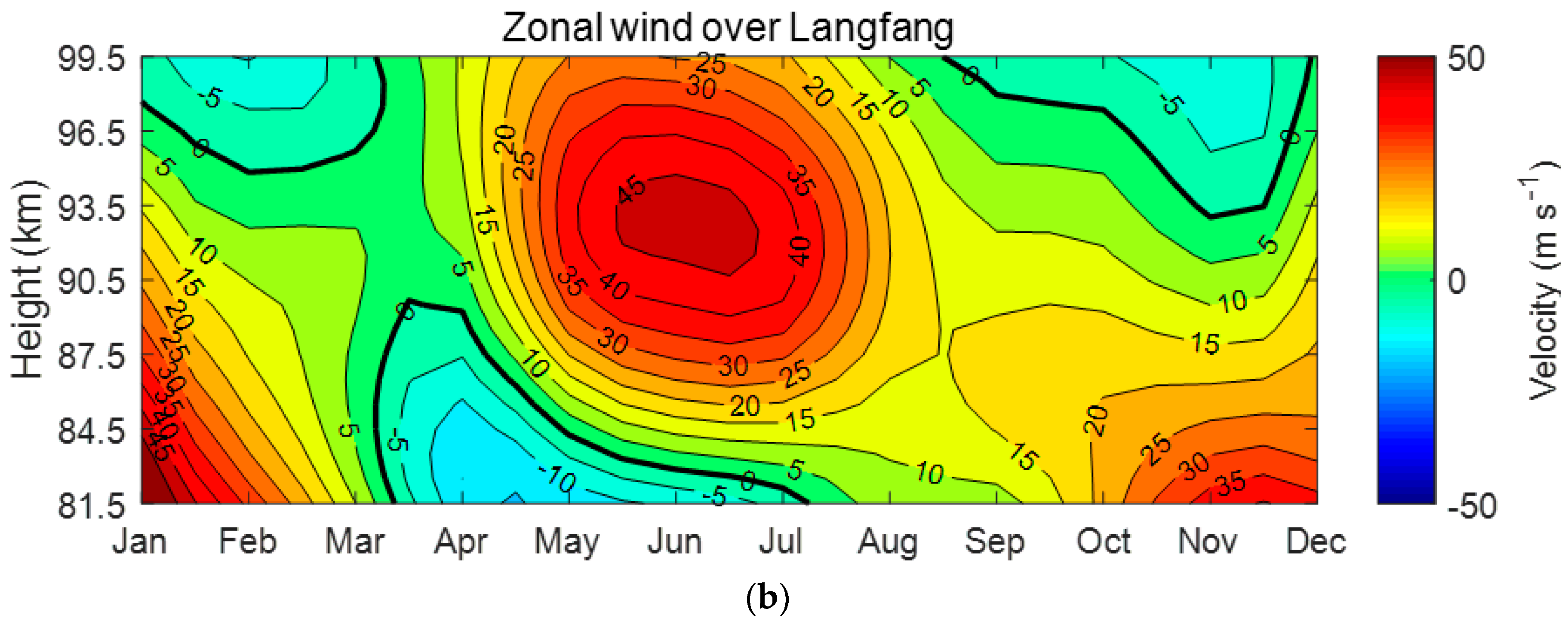
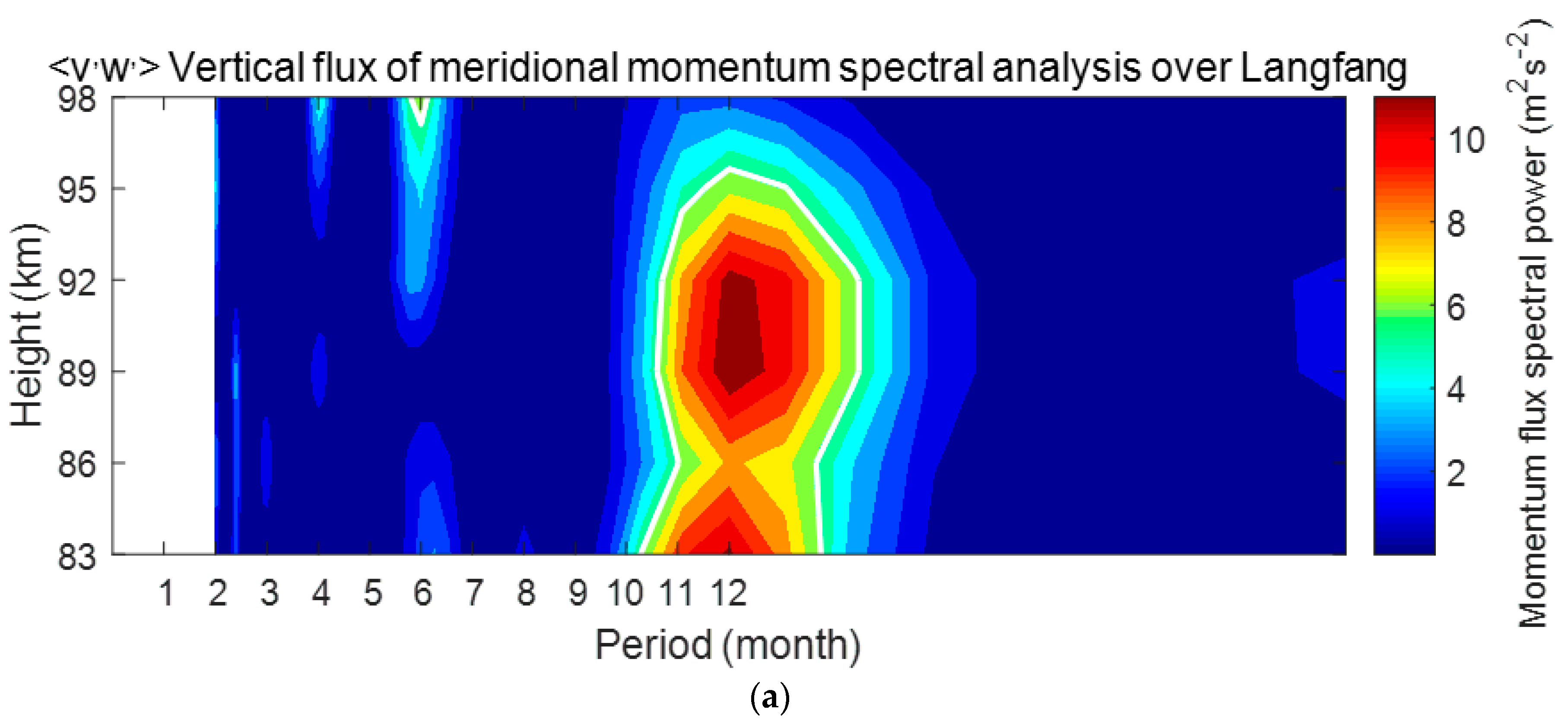
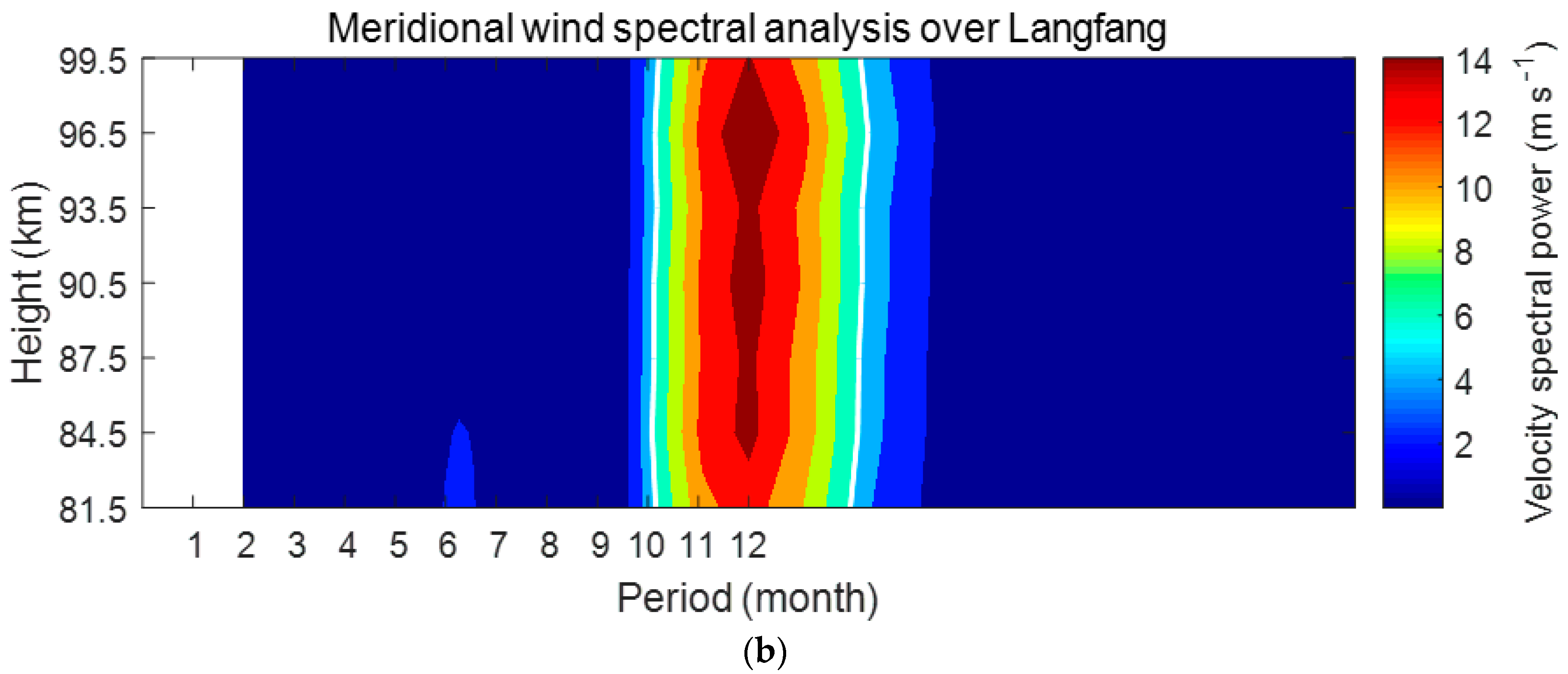
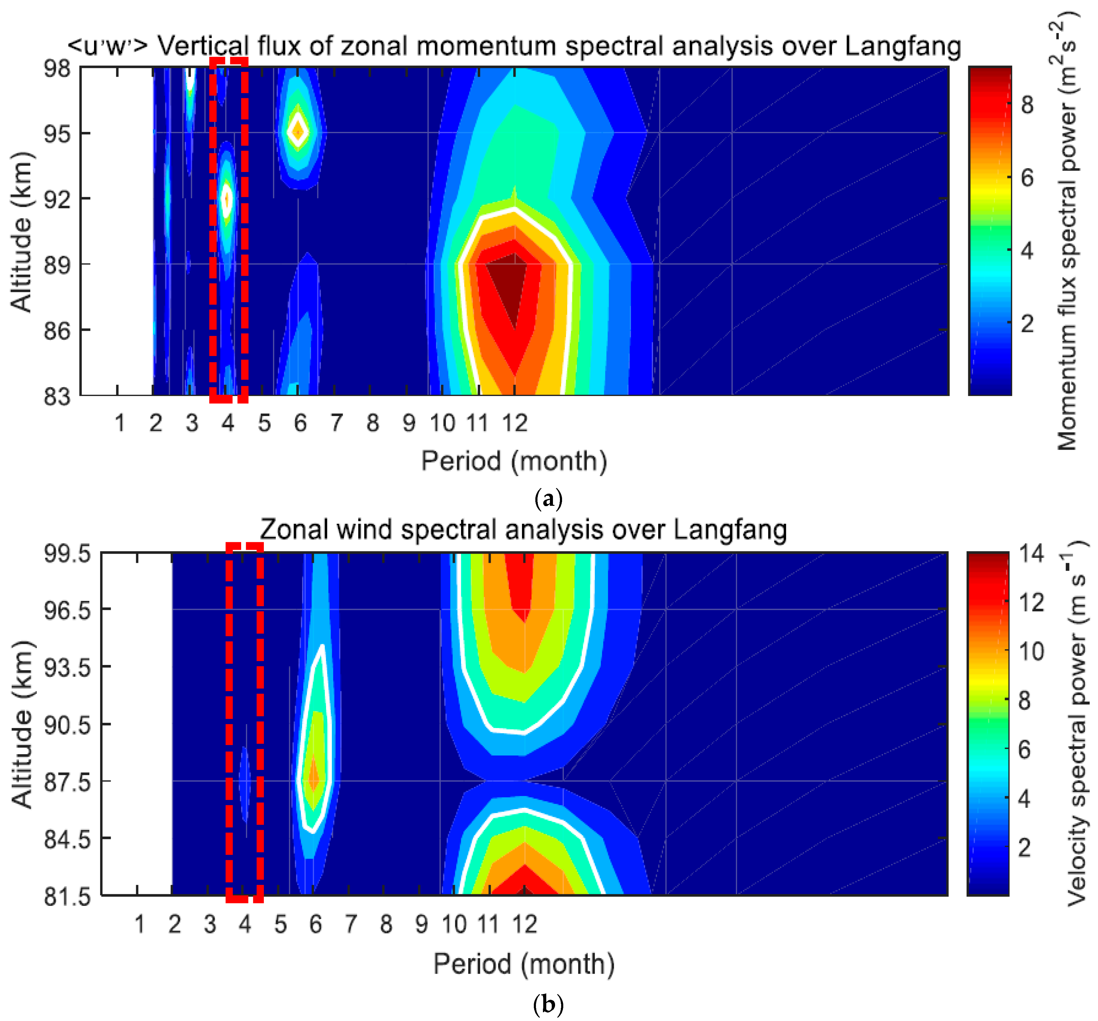
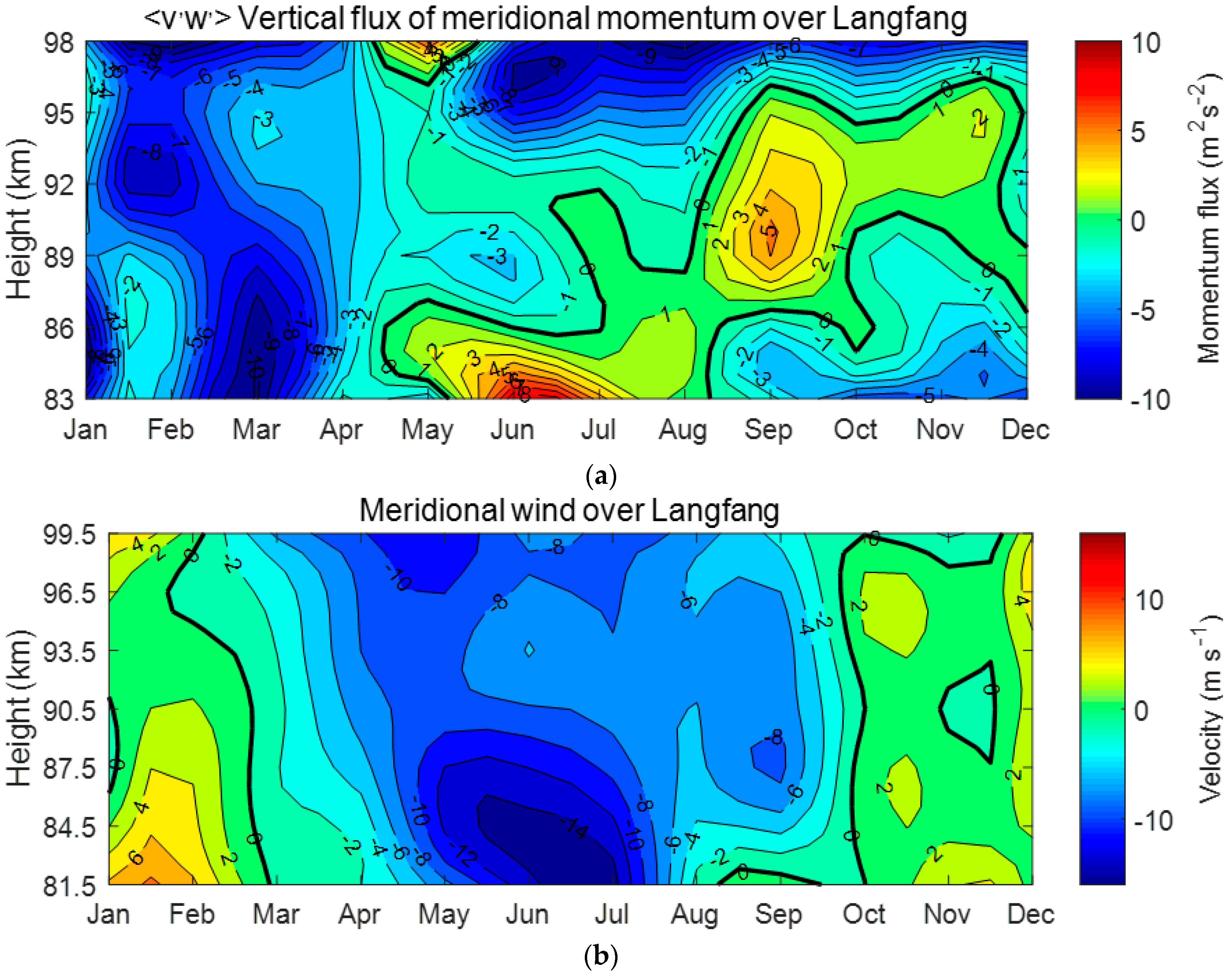
3.1. Momentum Flux of GW and its Seasonal Variation

GW momentum flux was calculated using an available data set acquired over Langfang from 1 July 2010 to 31 July 2011. Lomb-Scargle spectra were used to analyze monthly averages and vertical profiles in the zonal momentum flux, meridional momentum flux, zonal background wind, and meridional background wind. The height-time cross-sections of monthly averaged zonal momentum flux and zonal background wind are shown in Figure 1. Lomb-Scargle spectral analysis results for monthly averaged zonal momentum flux and zonal background wind are shown in Figure 2. Figure 3 shows the height-time cross-sections of monthly averaged meridional momentum flux and meridional background wind. Figure 4 shows the Lomb-Scargle spectral analysis results for monthly averaged meridional momentum flux and meridional background wind.

It is evident from Figure 1 and Figure 3 that the zonal momentum flux was directed primarily eastward, while the meridional momentum flux was mainly southward. Figure 1 shows that westward winds prevailed below the reversal height of the zonal wind in summer as the zonal momentum flux reached a maximum in the eastward direction. Figure 3 indicates that northward winds prevailed in winter and southward winds prevailed in summer. The meridional wind reached a maximum in the southward direction and the meridional momentum flux reached a maximum in the northward direction near 85 km in the summer.

Generally, GWs only continue to propagate upward when they move against the background wind. For example, due to the filtering effect of the background wind, most westward GWs can propagate vertically in eastward winds, while a few can propagate in westward winds. The background wind and momentum flux have opposite signs. When a westward (southward) wind prevails, the momentum flux is in the eastward (northward) direction and vice versa. GWs often break up near the mesopause (~87.5 km) as their amplitude increases exponentially with height. The resulting momentum is then applied to the background flow, causing a reversing force in the wind regime. Placke et al. also reported that zonal and meridional wind and momentum flux could be directly coupled in high- and low-latitude regions [12,13].

It is evident from Figure 1 and Figure 2 that monthly mean zonal winds exhibited a strong AO with a maximum occurring in the summer. SAO and quasi-4-month oscillations were also observed near the mesopause (~87.5 km). The quasi-4-month oscillation is consistent with the strong quasi-4-month oscillation of the zonal wind observed by Chen using medium frequency radar over Langfang [23]. In addition, the monthly mean momentum flux exhibited an AO with a maximum occurring in the summer and a SAO near the bottom and top. Quasi-4-month oscillations dominated near 92 km.

As shown in Figure 3 and Figure 4, the AO clearly dominated the monthly-mean meridional wind and fluxes. A weak SAO was only evident at the lower levels and quasi-4-month oscillations were negligible, which differed from monthly mean zonal winds. In addition, the meridional momentum flux exhibited a strong AO below ~95 km, SAO above ~92 km, and weak quasi-4-month oscillation above 95 km.

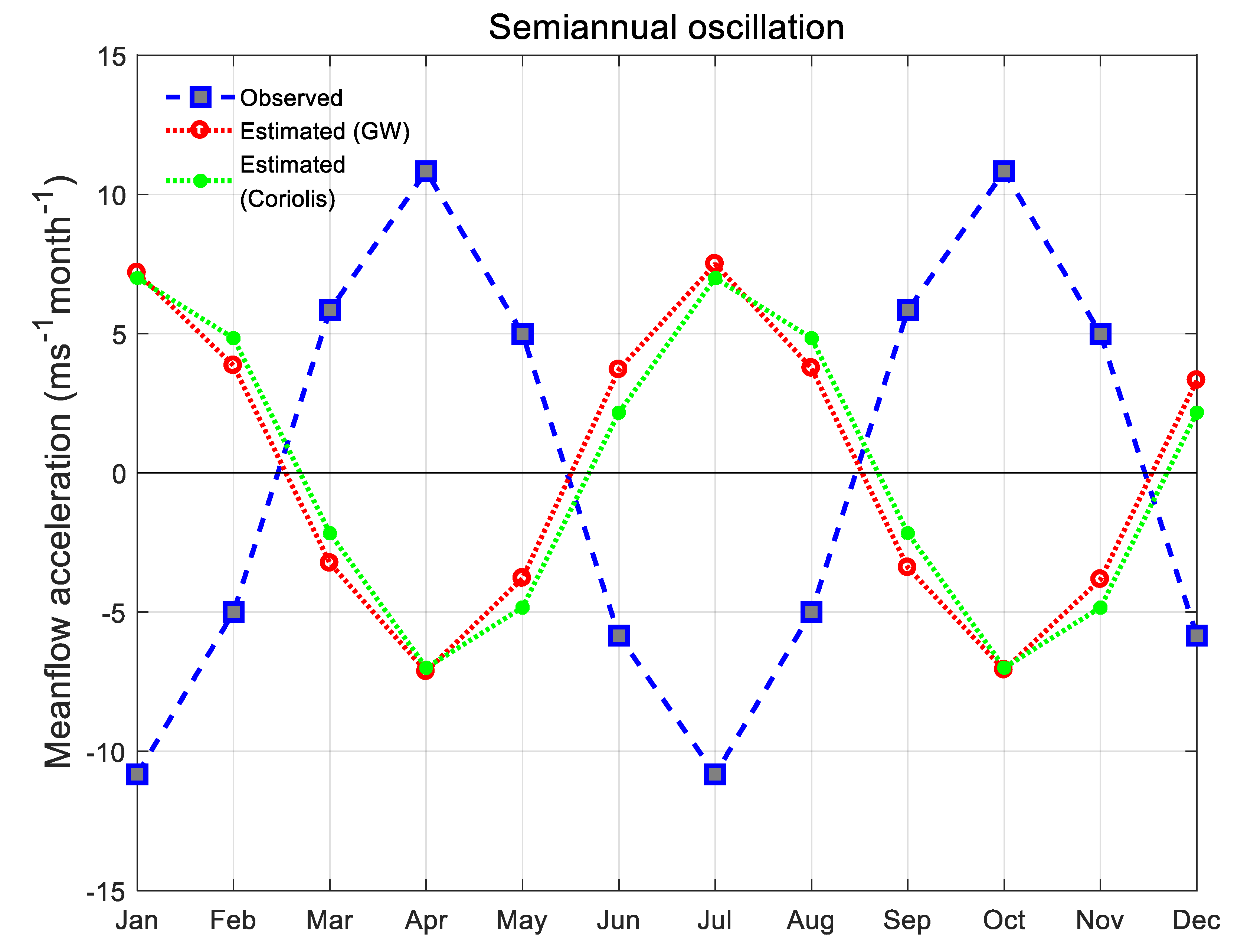
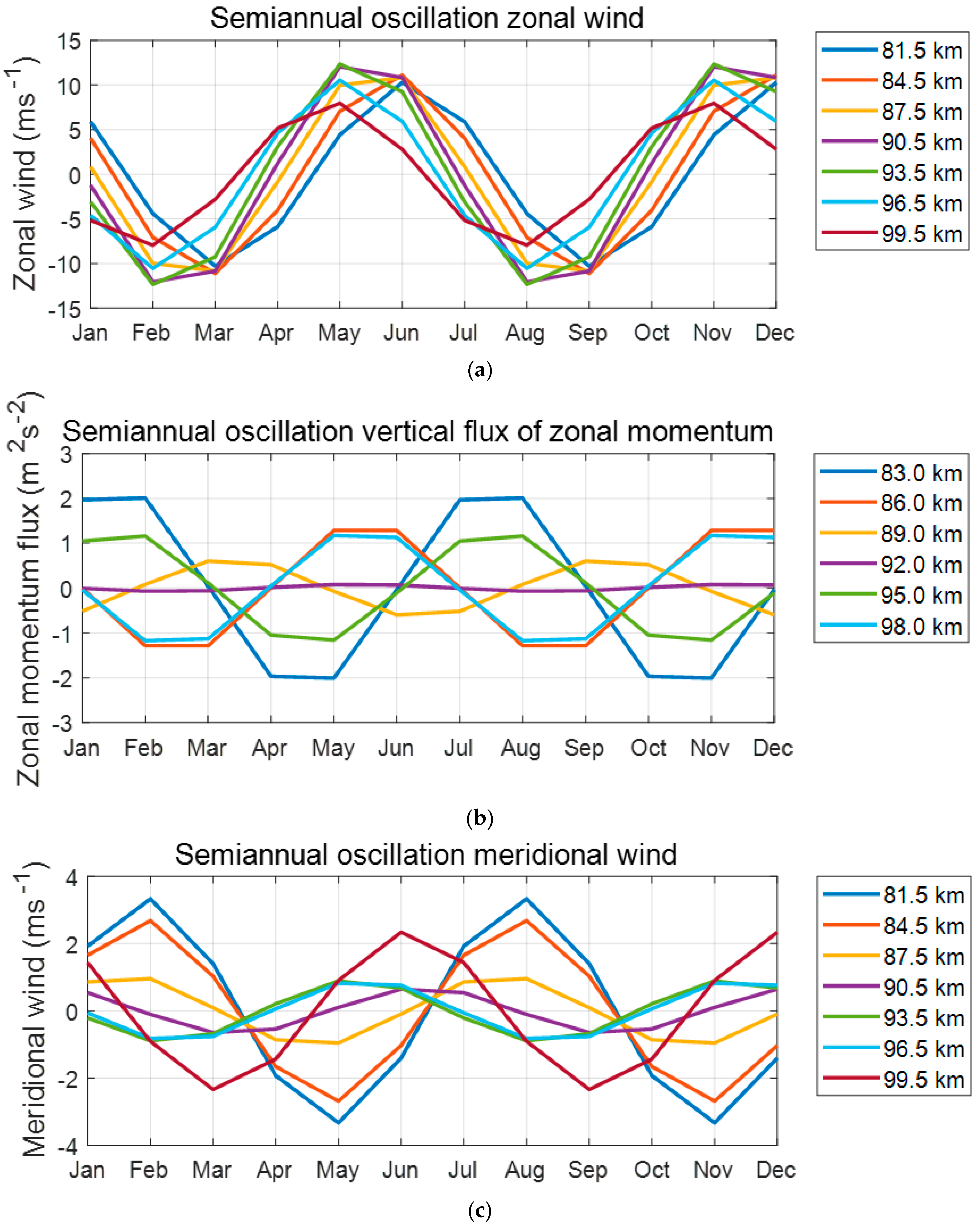
3.2. Observation and Estimation of Semi-Annual Oscillation Mean Flow Acceleration

Monthly mean background horizontal wind and monthly mean GW momentum flux were acquired using the data from the Langfang meteor radar. The SAO components of zonal wind, zonal momentum flux, and meridional wind were acquired using a harmonic fitting technique, as shown in Figure 5. A functional expression for SAO zonal wind was developed using a harmonic fit based on a Fourier transform and the observed acceleration was calculated by taking the derivative of the zonal wind speed. The average value of the observed acceleration was determined in the altitude direction, as indicated by the blue-dashed line in Figure 6. The estimated mean flow acceleration caused by deposition of SAO zonal momentum flux from high-frequency GWs was averaged in the altitude direction, as indicated by the red-dotted line in Figure 6. The estimated acceleration due to Coriolis forces was also averaged in the altitude direction, as denoted by the green-dotted line in Figure 6.

Table 1. Percentage of the contribution of gravity waves (GWs) and the Coriolis force to the SAO zonal wind.

Month	Observed Acceleration of SAO Zonal Wind	Estimated Acceleration from GW Momentum Fluxes	Estimated Acceleration due to Coriolis Force	Percentage of Contribution of GWs	Percentage of Contribution of Coriolis Force
January	−10.83	7.18	7.00	−66.30%	−64.62%
February	−4.99	3.85	4.83	−77.19%	−96.89%
March	5.84	−3.24	−2.16	−55.50%	−37.05%
April	10.83	−7.13	−7.00	−65.87%	−64.62%
May	4.99	−3.78	−4.83	−75.86%	−96.89%
June	−5.84	3.70	2.16	−63.42%	−37.05%
July	−10.83	7.50	7.00	−69.23%	−64.62%
August	−4.99	3.76	4.83	−75.35%	−96.89%
September	5.84	−3.40	−2.16	−58.25%	−37.05%
October	10.83	−7.08	−7.00	−65.33%	−64.62%
November	4.99	−3.83	−4.83	−76.69%	−96.89%
December	−5.84	3.32	2.16	−56.85%	−37.05%

shows the percentage of the contribution from the GW and Coriolis forces applied to the SAO zonal wind.

It is evident from Figure 6 and Table 1 that the estimated acceleration generated by GWs was in the opposite direction to the observed acceleration of the SAO zonal wind. In addition, the Coriolis force exerted an acceleration opposite to the observed acceleration of the SAO zonal wind. The action of other forces was required to balance the high-frequency GWs and Coriolis force. In this study, we used a 3-km height bin to remove variations with vertical scales of more than 3 km, and focused on the GWs with a vertical wavelength of less than 3 km. However, high-frequency GWs usually have long vertical wavelengths due to fast vertical phase speed. The force exerted by high-frequency GWs with vertical wavelengths of more than 3 km may have a great effect on the observed acceleration of the SAO zonal wind.

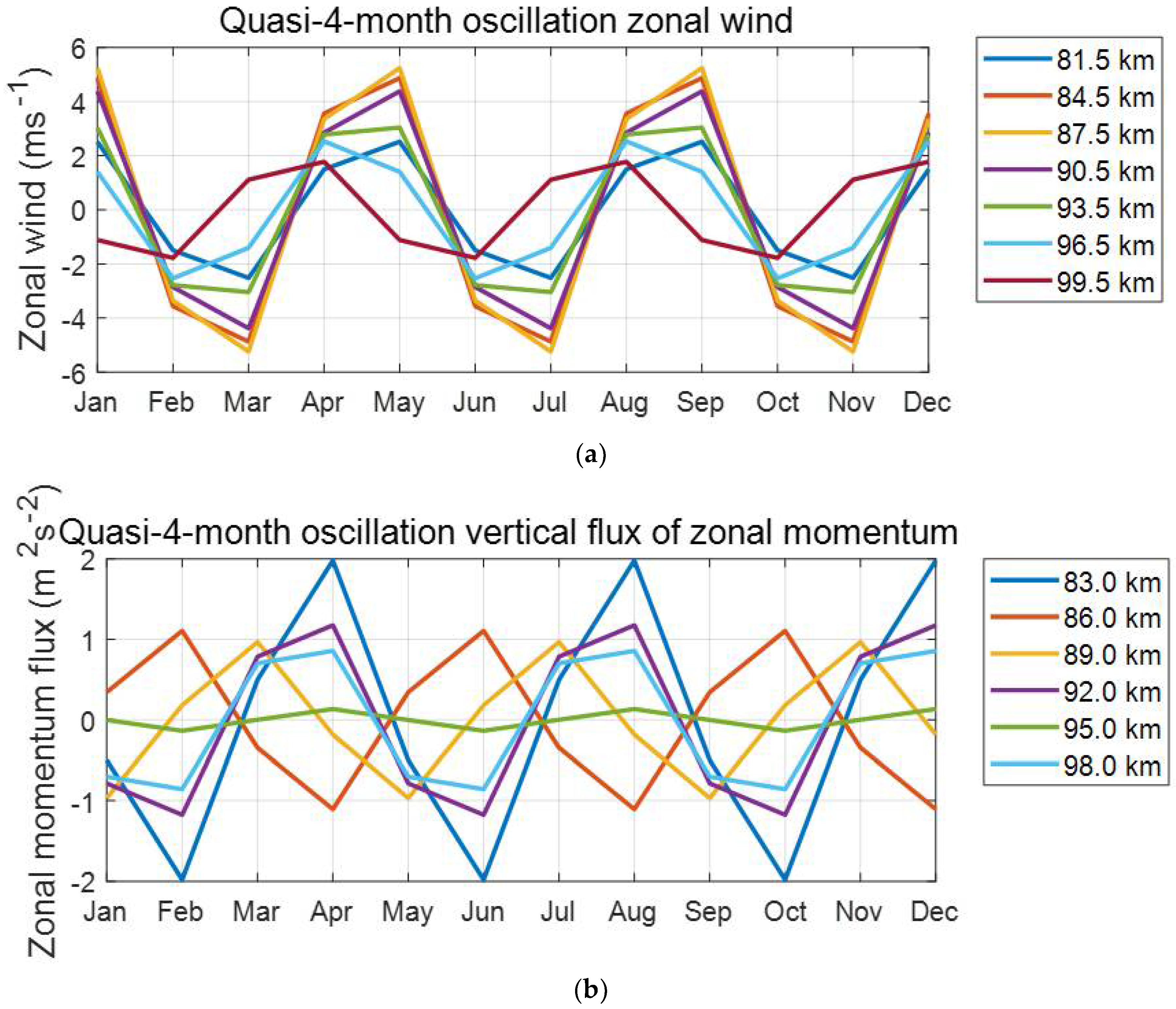
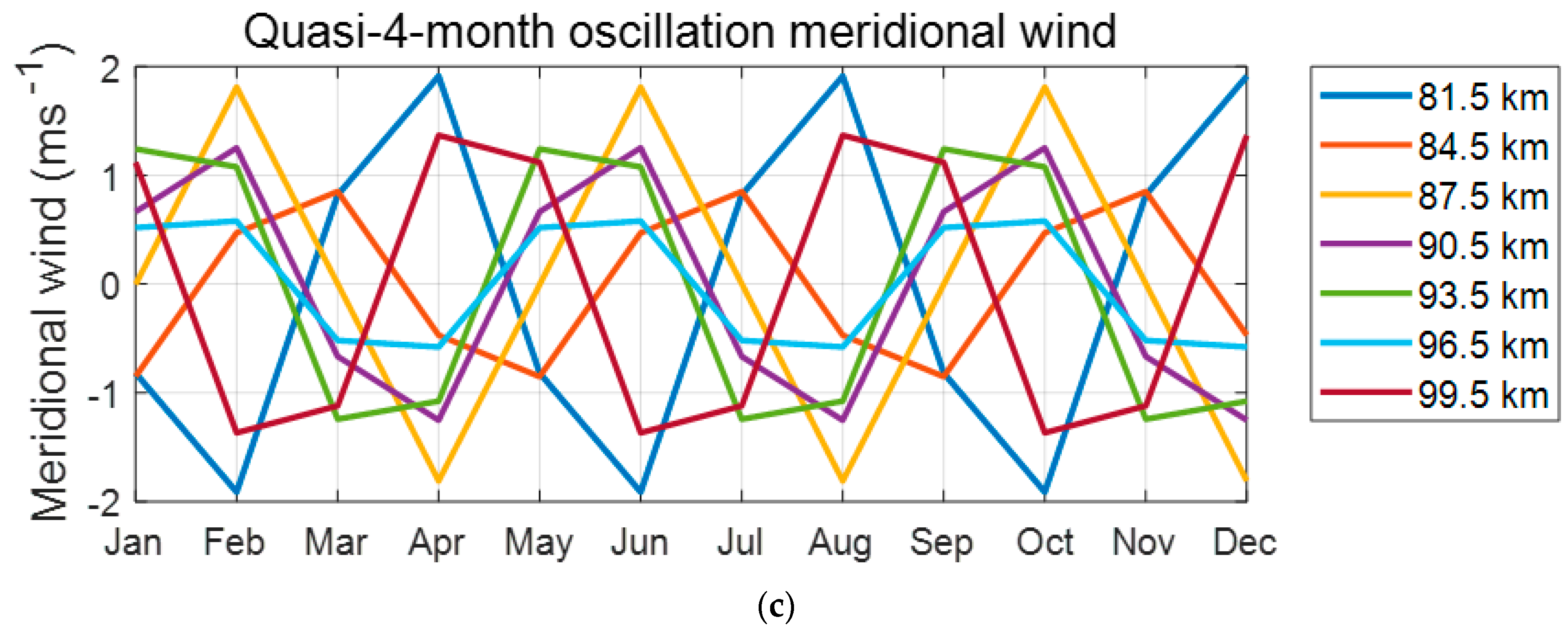
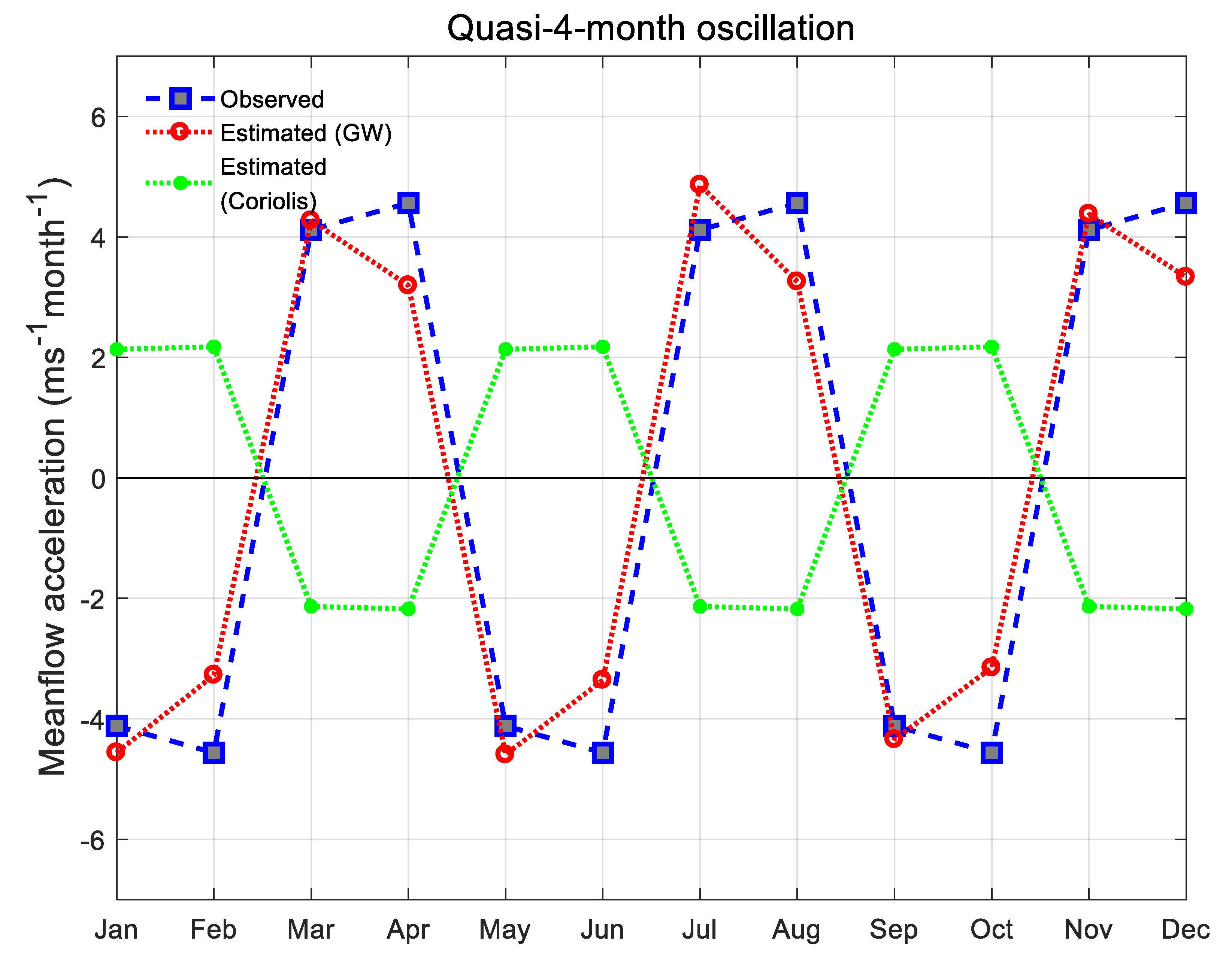
3.3. Observation and Estimation of Quasi-4-Month Oscillation Mean Flow Acceleration

Quasi-4-month oscillation components were acquired for the zonal wind, zonal momentum flux, and meridional wind using a harmonic fitting, as shown in Figure 7. A functional expression for the quasi-4-month oscillation zonal wind was developed using a Fourier transform. The observed acceleration was then calculated by taking the derivative of the zonal wind speed. The average value of observed acceleration was determined in the altitude direction, as represented by the blue-dashed line in Figure 8. The estimated mean flow acceleration caused by the deposition of quasi-4-month oscillation zonal momentum flux from high-frequency GWs was averaged in the altitude direction, as indicated by the red-dotted line in Figure 8. The estimated acceleration due to Coriolis forces was also averaged in the altitude direction, as denoted by the green-dotted line in Figure 8.

Table 2. Percentage of the contribution of GWs and the Coriolis force to the quasi-4-month oscillation zonal wind.

Month	Observed Acceleration of Quasi-4-Month Oscillation Zonal Wind	Estimated Acceleration from GW Momentum Fluxes	Estimated Acceleration due to Coriolis Force	Percentage of Contribution of GWs	Percentage of Contribution of Coriolis Force
January	−4.12	−4.56	2.13	110.76%	−51.84%
February	−4.56	−3.27	2.18	71.73%	−47.69%
March	4.12	4.27	−2.13	103.74%	−51.84%
April	4.56	3.19	−2.18	69.97%	−47.69%
May	−4.12	−4.59	2.13	111.57%	−51.84%
June	−4.56	−3.36	2.18	73.58%	−47.69%
July	4.12	4.86	−2.13	118.06%	−51.84%
August	4.56	3.26	−2.18	71.39%	−47.69%
September	−4.12	−4.34	2.13	105.44%	−51.84%
October	−4.56	−3.15	2.18	69.06%	−47.69%
November	4.12	4.38	−2.13	106.38%	−51.84%
December	4.56	3.33	−2.18	73.03%	−47.69%

shows the percentage of the contribution from the GWs and Coriolis forces to the quasi-4-month oscillation zonal wind.

It is evident from Figure 8 and Table 2 that the estimated acceleration generated by GWs was in the same direction as the observed acceleration of the quasi-4-month oscillation zonal wind, and there is a high correlation. In February, April, June, August, October, and December, the estimated acceleration from the divergence of zonal momentum flux from GWs contributed more than 69% to the observed acceleration. In January, March, May, July, September, and November, the estimated acceleration from GWs was greater than the observed acceleration; additional forces (such as the Coriolis force) were needed to achieve equilibrium. The estimated acceleration due to the Coriolis force opposed the estimated acceleration from high-frequency GWs, thus the force of the high-frequency GWs offset the Coriolis force.

4. Discussion

4.1. Error Analysis

4.1.1. Momentum Flux Determination

A dual beam technique for calculating momentum flux was first introduced by Reid and Vincent [32]. Hocking later generalized this dual beam formulation and used meteor radar data from mid-latitude and polar sites to measure momentum flux. An average interval of less than 3 h was used in any height/time bin, suggesting the determination of momentum flux is caused by GWs with a period of less than 2–3 h, after removing contamination from tides and planetary waves [10]. Subsequently, multiple studies have examined the reliability of this technique and have proposed improvements. For example, Placke et al. considered the contamination from vertical wind shear and used a correction term to minimize the resulting error [13]. Andrioli et al. analyzed meteor radar data from Brazil, and demonstrated that composite days (averaged over multiple days) could be used to remove tidal effects. However, residual tidal components caused by day-to-day variability can still contaminate the calculated momentum flux [25]. Liu et al. analyzed this method using meteor radar wind measurements at Maui, Hawaii (20.7° N, 156.3° W) and derived diurnal variations for GW momentum flux by constructing a composite day in every calendar month. The group used five years of data from Maui, but they did not use the correlation formula developed by Placke et al. to minimize errors from vertical wind shear. Rather, they simply employed interpolation to acquire a more accurate mean background wind and a projected mean radial velocity, which was then subtracted from the measured radial velocity to calculate perturbations caused by GWs and minimize errors due to vertical wind shear [13,14].

In this study, the background wind that we removed included day-to-day tidal variations, as we are not using a composite method to determine tides. We simply removed variations with periods longer than 2 h and vertical scales longer than 3 km. As such, there is no tidal contamination issue as described in Andrioli et al. [25]. Besides, linear interpolation in height and time was used to resolve vertical and temporal shear information in the background wind. This approach avoids contamination due to vertical wind shear, as described by Placke et al. [13]. Furthermore, as mentioned by Spargo et al., measures were taken to remove outliers that biased momentum flux results; in the first step, meteors with radial velocities of more than 200 m/s were discarded, and, in the second step, a 5-standard-deviations criterion was used to remove outliers [29].

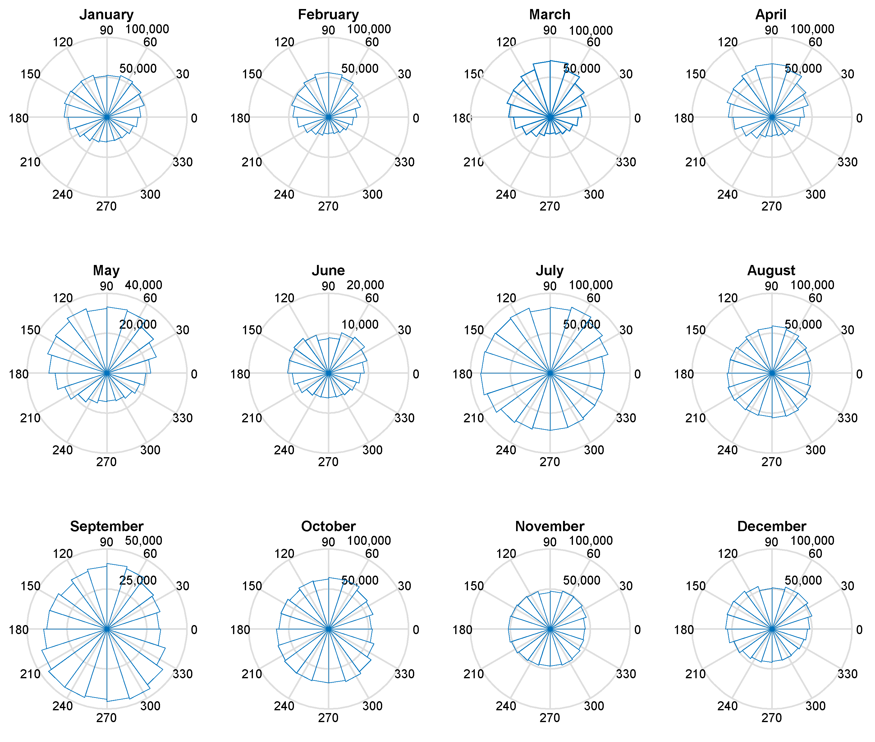
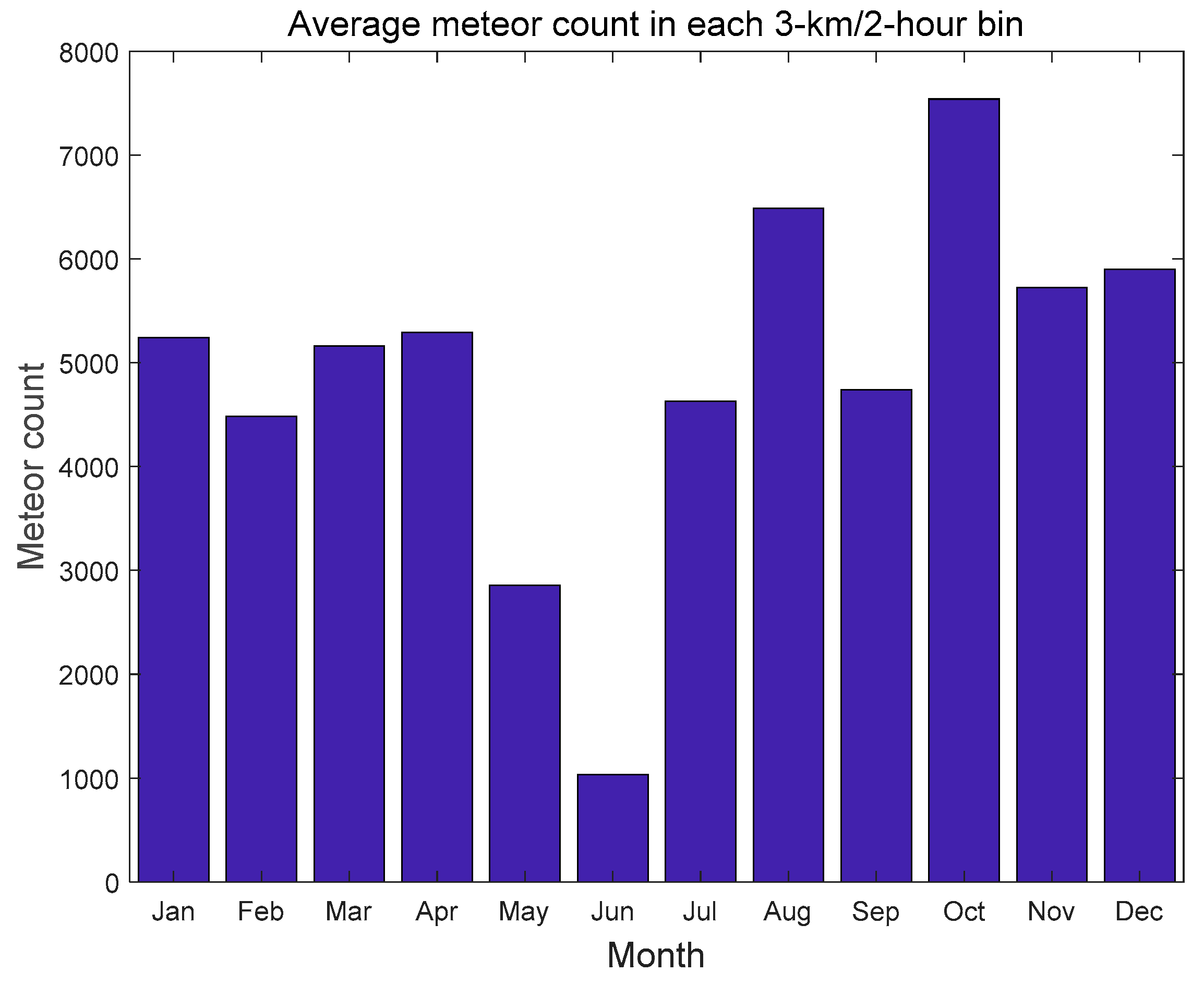
4.1.2. Meteor Statistics

Hocking proposed that detecting 30 meteors within an hour was sufficient for measuring momentum flux [10]. Vincent et al. employed a Monte Carlo technique to investigate the influence of meteor counts in estimating short-period GW activity using Hocking’s method. The resulting meteor data suggested that averaging over one month was required to obtain meaningful values for momentum flux, as meteor counts also affected the uncertainty [28].

In this study, only meteors with a zenith angle between 15° and 60°, and a height between 80 and 101 km, were included in the data. A composite day was then established for every month. Average meteor counts in each 3-km and 2-h bin are shown for each composite day in Figure 9. The average meteor count in each time/height bin reached a minimum in June and peaked in October, and exceeded 3000 in most months. The calculation error for background wind and GW momentum flux was small as there were enough meteor counts in each time/height bin.

Figure 10 shows the azimuthal distribution of total meteor detections for every composite day in each calendar month. These counts are higher than those acquired in Maui, as described by Liu et al., or in Beijing, as described by Jia et al. [14,20]. There were slightly more meteors detected in the northwest of Langfang from January to June (and July and December). More meteors were detected in the southwest of Langfang from August to November. The primary reason for this discrepancy was the antenna alignment [14], which was also affected by the latitude of the meteor radar site and the geographic conditions near the radar antenna. Since azimuthal variations in meteor count rates were relatively small, their influence on the calculation of background wind and GW momentum flux could be ignored.

4.2. Seasonal Variation of GW Momentum Flux

The observed seasonal variations in zonal momentum flux over different stations at varying latitudes differed significantly. The specific stations and their corresponding characteristics can be described as follows. (1) In Mohe (53.5° N, 122.3° E), an AO occurred above 90 km. Flux was directed eastward in the winter and spring and westward in the summer and autumn [20]. (2) In Beijing (40.3° N, 116.2° E), an AO occurred above 92 km with a minimum amplitude in summer and a maximum amplitude in winter. A weak SAO occurred below 87 km, and reached its maximum value in January-March and August-October [20]. (3) In Mengcheng (33.3° N, 116.5° E), an AO was observed above 90 km with a negative maximum value in summer and a negative minimum value in winter [20]. (4) In Wuhan (30.5° N, 114.2° E), there was no obvious periodic variation [20]. (5) In Tirupati (13.63° N, 79.4° E), a SAO occurred below 90 km and was directed eastward near equinoxes and westward near solstices [21]. (6) Thumba (8.5° N, 77° E) detected a SAO below 90 km [21]. (7) At Biak (1.17° S, 136.10° E), a SAO occurred at 86–92 km and was most obvious at the upper and lower altitudes [19]. (8) In Kototabang (0.2° S, 100.3° E), a SAO occurred below 90 km and was directed westward near equinoxes and eastward near solstices [21]. (9) At Cariri (7° S, 36° W), an AO occurred at 89 and 92.5 km, with a maximum value in June [15]. (10) Similarly, in Cachoeira Paulista (23° S, 45° W), an AO occurred at 89 and 92.5 km, with a maximum value in June [15]. (11) In Santa Maria (30° S, 54° W), an AO only occurred at 92.5 km, with a maximum value in June. Quasi-4-month oscillations also occurred at 92.5 km [15].

As with zonal momentum flux, meridional momentum flux exhibited geographical differences. The specific stations and their corresponding characteristics can be described as follows. (1) In Mohe (53.5° N, 122.3° E), an AO occurred above 78–87 km, and was directed southward during the first half of the year and northward during the second half of the year [20]. (2) Similarly, an AO was observed in Beijing (40.3° N, 116.2° E) and was directed southward during the first half of the year and northward during the second half of the year [20]. (3) In Mengcheng (33.3° N, 116.5° E), an AO occurred above 78–87 km and was directed southward during the first half of the year and northward during the second half of the year [20]. (4) In Wuhan (30.5° N, 114.2° E), an AO occurred throughout the year, reaching a southward maximum in March and a southward minimum in July [20]. (5) In Tirupati (13.63° N, 79.4° E), a quasi-4-month oscillation occurred below 90 km [21]. (6) In Thumba (8.5° N, 77° E), a SAO occurred in a northward direction near equinoxes and displayed a weak southward momentum flux near solstices [21]. (7) In Biak (1.17° S, 136.10° E), an AO occurred above 90 km [19]. (8) In Kototabang (0.2° S, 100.3° E), a SAO occurred below 88 km [21]. (9) Data from Cariri (7° S, 36° W) exhibited no obvious periodic variation [15]. (10) In Cachoeira Paulista (23° S, 45° W), a quasi-4-month oscillation occurred at 92.5 km, and reached a maximum in February, June, and October [15]. (11) In Santa Maria (30° S, 54° W), an AO occurred at 89 km with a maximum value in the winter [15].

The following can be inferred from the momentum flux observations discussed above. (1) The AO was more pronounced in mid-latitude regions and weaker in low-latitudes and equatorial regions. (2) The SAO was weak in mid-latitudes and only strong near the equator. Zonal momentum flux was directed eastward near the equinoxes (with northward meridional winds) and westward near the solstices (with southward meridional winds). (3) Quasi-4-month oscillations have been observed in both mid-latitude and low-latitude regions. Andrioli et al. found evidence of quasi-4-month oscillations in zonal momentum flux [15], which is in agreement with this study. In addition, both Andrioli et al. and Pramitha et al. reported quasi-4-month oscillations in the meridional momentum flux [15,21], which were weak enough over the Langfang station to be ignored in this study.

4.3. Mean Flow Acceleration

The estimated acceleration generated by a high-frequency GW (with a vertical wavelength of less than 3 km) momentum flux was in the opposite direction, with the observed acceleration of SAO zonal winds in the MLT region over Langfang. Antonita et al. used meteor radar data to estimate GW momentum flux over Trivandrum (8.5° N, 76.9° E) and determined that the contribution of high-frequency GW momentum flux to the mesosphere semiannual oscillation (MSAO) was 20–70%. They also suggested that the deviation between the estimated acceleration of GW momentum flux and the observed acceleration of the MSAO may be due to the contribution of planetary waves, inertial GWs, and tidal waves [11]. Langfang is in a mid-latitude region while Trivandrum is located near the Equator. As such, high-frequency GW momentum flux contributed less to the SAO of zonal winds in Langfang than in Trivandrum, which may be due to the different intensities of atmospheric GWs in equatorial and mid-latitude regions [33,34]. In Langfang, the contribution of high-frequency GWs (with a vertical wavelength of less than 3 km) to the SAO zonal wind is relatively small, and other contributions, including high-frequency GWs (with a vertical wavelength of more than 3 km), inertial GWs, planetary waves, and tidal waves need to be studied further.

The contribution of high-frequency GWs to the acceleration of quasi-4-month oscillation zonal winds in the MLT region over Langfang was 71.73%, 69.97%, 73.58%, 71.39%, 69.06%, and 73.03% in February, April, June, August, October, and December, respectively. High-frequency GWs played a key role in quasi-4-month oscillation zonal winds. In January, March, May, July, September, and November, the estimated acceleration of the high-frequency GWs exceeded the observed acceleration of quasi-4-month oscillation zonal winds, and the contribution of other forces, such as planetary waves, inertial gravity waves, tides, and the Coriolis force, may play a balancing role.

In this study, the estimated acceleration of the Coriolis force on SAO and quasi-4-month oscillation zonal wind is given. At the mesopause, Coriolis forces deflect meridional winds as the earth rotates, forming zonal winds. If there are no other forces, the zonal winds will become stronger and stronger, and there must be counteracting forces to balance the Coriolis forces. For SAO zonal winds, high-frequency GWs were not sufficient to counteract the effect of the Coriolis force, and other forces contribute, such as inertial GWs. For the quasi-4-month oscillation zonal wind, the acceleration produced by the Coriolis force was found to be opposite to the estimated acceleration of high-frequency GWs, which verifies the mechanism of the effect of GWs counteracting the Coriolis force. For quasi-4-month oscillations zonal winds, the high-frequency GWs were strong enough to counteract the Coriolis force.

The data used in this study were acquired from July 1, 2010 to July 31, 2011. The calculated acceleration of zonal winds and mean meridional wind were an average of values collected at a single station, as opposed to a zonal average. However, the monthly average zonal wind acceleration at single stations represented zonal averages and the corresponding conclusions were limited to a specific region and year.

5. Conclusions

In this study, Hocking’s technique was used to determine high-frequency GW momentum flux and estimate the contribution of high-frequency GWs to the SAO in zonal winds. A relationship between high-frequency GWs and quasi-4-month oscillation zonal winds was established for the first time. The following conclusions were drawn from the meteor radar data acquired at Langfang, China (39.4° N, 116.7° E) from 1July 2010 to 31 July 2011.

First, seasonal variations were identified in the momentum flux of GWs with periods of less than 2 h at ~40° N in the MLT region. Zonal momentum flux exhibited AO with a maximum occurring in the summer and SAO near the bottom and top of the altitude range. Quasi-4-month oscillations dominated near 95 km. Meridional momentum flux exhibited strong AO below ~95 km, SAO above ~92 km, and weak quasi-4-month oscillations above 95 km. Second, the estimated acceleration generated by high-frequency GWs with a vertical wavelength of less than 3 km and the observed acceleration of SAO zonal winds were in opposite directions. Third, high-frequency GWs played a key role in the quasi-4-month oscillation of zonal winds, with a contribution of more than 69% in February, April, June, August, October, and December. The contributions from high-frequency GWs in these months were 71.73%, 69.97%, 73.58%, 71.39%, 69.06%, and 73.03%, respectively. In January, March, May, July, September, and November, the estimated acceleration of high-frequency GWs exceeded the observed acceleration of zonal winds, and Coriolis forces were found to play a major balancing role. Fourth, the estimated acceleration due to Coriolis forces to zonal winds was studied. The forces of high-frequency GWs and the Coriolis force were in opposite directions for a quasi-4-month oscillation zonal wind, and in the same direction for a SAO zonal wind. Fifth, in addition to GW deposition and Coriolis forces, additional waves contributed to the mean flow acceleration. These included tidal waves, planetary waves, and inertial GWs, which should be investigated further in a future study.

References

1. Taylor, M.J.; Hapgood, M.A. Identification of a thunderstorm as a source of short period gravity waves in the upper atmospheric nightglow emissions. Planet. Space Sci. 1988, 36, 975–985. [Google Scholar] [CrossRef]
2. Lindzen, R.S. Turbulence and stress owing to gravity-wave and tidal breakdown. J. Geophys. Res. 1981, 86, 9707–9714. [Google Scholar] [CrossRef] [Green Version]
3. Fritts, D.C.; Vincent, R.A. Mesospheric momentum flux studies at adelaide, australia: Observations and a gravity wave–tidal interaction model. J. Atmos. Sci. 1987, 44, 605–619. [Google Scholar] [CrossRef] [Green Version]
4. Geller, M.A.; Alexander, M.J.; Love, P.T.; Bacmeister, J.; Ern, M.; Hertzog, A.; Manzini, E.; Preusse, P.; Sato, K.; Scaife, A.A.; et al. A comparison between gravity wave momentum fluxes in observations and climate models. J. Clim. 2013, 26, 6383–6405. [Google Scholar] [CrossRef] [Green Version]
5. Placke, M.; Hoffmann, P.; Latteck, R.; Rapp, M. Gravity wave momentum fluxes from MF and meteor radar measurements in the polar MLT region. Geophys. Res. Space 2015, 120, 736–750. [Google Scholar] [CrossRef] [Green Version]
6. Suzuki, S.; Shiokawa, K.; Otsuka, Y.; Ogawa, T.; Kubota, M.; Tsutsumi, M.; Nakamura, T.; Fritts, D.C. Gravity wave momentum flux in the upper mesosphere derived from oh airglow imaging measurements. Earth Planets Space 2007, 59, 421–428. [Google Scholar] [CrossRef] [Green Version]
7. Espy, P.J.; Jones, G.O.L.; Swenson, G.R.; Tang, J.; Taylor, M.J. Seasonal variations of the gravity wave momentum flux in the antarctic mesosphere and lower thermosphere. J. Geophys. Res. 2004, 109, D23109. [Google Scholar] [CrossRef] [Green Version]
8. Acott, P.E.; She, C.-Y.; Krueger, D.A.; Yan, Z.-A.; Yuan, T.; Yue, J.; Harrell, S. Observed nocturnal gravity wave variances and zonal momentum flux in mid-latitude mesopause region over Fort Collins, Colorado, USA. J. Atmos. Sol. Terr. Phys. 2011, 73, 449–456. [Google Scholar] [CrossRef]
9. Li, T.; Ban, C.; Fang, X.; Li, J.; Wu, Z.; Feng, W.; Plane, J.M.C.; Xiong, J.; Marsh, D.R.; Mills, M.J.; et al. Climatology of mesopause region nocturnal temperature, zonal wind, and sodium density observed by sodium lidar over Hefei, China (32° N, 117° E). Atmos. Chem. Phys. 2018, 18, 11683–11695. [Google Scholar] [CrossRef] [Green Version]
10. Hocking, W.K. A new approach to momentum flux determinations using SKiYMET meteor radars. Ann. Geophys. 2005, 23, 2433–2439. [Google Scholar] [CrossRef] [Green Version]
11. Antonita, T.M.; Ramkumar, G.; Kumar, K.K.; Deepa, V. Meteor wind radar observations of gravity wave momentum fluxes and their forcing toward the mesospheric semiannual oscillation. J. Geophys. Res. Atmos. 2008, 113. [Google Scholar] [CrossRef] [Green Version]
12. Placke, M.; Hoffmann, P.; Becker, E.; Jacobi, C.; Singer, W.; Rapp, M. Gravity wave momentum fluxes in the MLT—Part II: Meteor radar investigations at high and midlatitudes in comparison with modeling studies. J. Atmos. Sol. Terr. Phys.. 2011, 73, 911–920. [Google Scholar] [CrossRef]
13. Placke, M.; Stober, G.; Jacobi, C. Gravity wave momentum fluxes in the MLT—Part I: Seasonal variation at Collm (51.3° N, 13.0° E). J. Atmos. Sol. Terr. Phys. 2011, 73, 904–910. [Google Scholar] [CrossRef]
14. Liu, A.Z.; Lu, X.; Franke, S.J. Diurnal variation of gravity wave momentum flux and its forcing on the diurnal tide. J. Geophys. Res. Atmos. 2013, 118, 1668–1678. [Google Scholar] [CrossRef] [Green Version]
15. Andrioli, V.F.; Batista, P.P.; Clemesha, B.R.; Schuch, N.J.; Buriti, R.A. Multi-year observations of gravity wave momentum fluxes at low and middle latitudes inferred by all-sky meteor radar. Ann. Geophys. 2015, 33, 1183–1193. [Google Scholar] [CrossRef] [Green Version]
16. de Wit, R.J.; Hibbins, R.E.; Espy, P.J.; Orsolini, Y.J.; Limpasuvan, V.; Kinnison, D.E. Observations of gravity wave forcing of the mesopause region during the January 2013 major Sudden Stratospheric Warming. Geophys. Res. Lett. 2014, 41, 4745–4752. [Google Scholar] [CrossRef] [Green Version]
17. De Wit, R.; Hibbins, R.; Espy, P.J. The seasonal cycle of gravity wave momentum flux and forcing in the high latitude northern hemisphere mesopause region. J. Atmos. Sol. Terr. Phys. 2015, 127, 21–29. [Google Scholar] [CrossRef]
18. Moss, A.C.; Wright, C.J.; Davis, R.N.; Mitchell, N.J. Gravity-wave momentum fluxes in the mesosphere over Ascension Island (8° S, 14° W) and the anomalous zonal winds of the semi-annual oscillation in 2002. Ann. Geophys. 2016, 34, 323–330. [Google Scholar] [CrossRef] [Green Version]
19. Matsumoto, N.; Shinbori, A.; Riggin, D.M.; Tsuda, T. Measurement of momentum flux using two meteor radars in Indonesia. Ann. Geophys. 2016, 34, 369–377. [Google Scholar] [CrossRef] [Green Version]
20. Jia, M.; Xue, X.; Gu, S.-Y.; Chen, T.; Ning, B.; Wu, J.; Zeng, X.; Dou, X.; Mingjiao, J.; Xianghui, X.; et al. Multi-year observations of gravity wave momentum fluxes in the mid-latitude mesosphere and lower thermosphere region by meteor radar. J. Geophys. Res. Space Phys. 2018, 123, 5684–5703. [Google Scholar] [CrossRef] [Green Version]
21. Pramitha, M.; Kumar, K.K.; Ratnam, M.V.; Rao, S.V.B.; Ramkumar, G. Meteor radar estimations of gravity wave momentum fluxes: Evaluation using simulations and observations over three tropical locations. J. Geophys. Res. Space Phys. 2019, 124, 7184–7201. [Google Scholar] [CrossRef]
22. de Wit, R.J.; Janches, D.; Fritts, D.C.; Hibbins, R.E. QBO modulation of the mesopause gravity wave momentum flux over Tierra del Fuego. Geophys. Res. Lett. 2016, 43, 4049–4055. [Google Scholar] [CrossRef] [Green Version]
23. Chen, X. Researches on the Variations of the Mesospheric and Thermospheric Atmosphere; Degree-University of Chinese Academy of Sciences: Beijing, China, 2013. [Google Scholar]
24. Iimura, H.; Fritts, D.C.; Riggin, D.M. Long-term oscillations of the wind field in the tropical mesosphere and lower thermosphere from Hawaii MF radar measurements. J. Geophys. Res. Atmos. 2010, 115. [Google Scholar] [CrossRef]
25. Andrioli, V.F.; Fritts, D.C.; Batista, P.P.; Clemesha, B.R. Improved analysis of all-sky meteor radar measurements of gravity wave variances and momentum fluxes. Ann. Geophys. 2013, 31, 889–908. [Google Scholar] [CrossRef] [Green Version]
26. Fritts, D.C.; Janches, D.; Iimura, H.; Hocking, W.K.; Bageston, J.V.; Leme, N.M.P. Drake antarctic agile meteor radar first results: Configuration and comparison of mean and tidal wind and gravity wave momentum flux measurements with Southern Argentina Agile Meteor Radar. J. Geophys. Res. Atmos. 2012, 117, D02105. [Google Scholar] [CrossRef] [Green Version]
27. Holdsworth, D.A.; Reid, I.M.; Cervera, M.A. Buckland Park all-sky interferometric meteor radar. Radio Sci. 2004, 39, RS5009. [Google Scholar] [CrossRef]
28. Vincent, R.A.; Kovalam, S.; Reid, I.M.; Younger, J.P. Gravity wave flux retrievals using meteor radars. Geophys. Res. Lett. 2010, 37, 37. [Google Scholar] [CrossRef]
29. Spargo, A.J.; Reid, I.M.; MacKinnon, A.D. Multistatic meteor radar observations of gravity-wave-tidal interaction over southern Australia. Atmos. Meas. Tech. 2019, 12, 4791–4812. [Google Scholar] [CrossRef] [Green Version]
30. Fritts, D.C.; Alexander, M.J. Gravity wave dynamics and effects in the middle atmosphere. Rev. Geophys. 2003, 41. [Google Scholar] [CrossRef] [Green Version]
31. Andrews, D.G.; Holton, J.R.; Leovy, C.B. Middle Atmosphere Dynamics; Academic Press: Orlando, FL, USA; San Diego, CA, USA; New York, NY, USA, 1987; pp. 8–128. [Google Scholar]
32. Reid, I.M.; Vincent, R.A. Measurements of mesospheric gravity wave momentum fluxes and mean flow accelerations at Adelaide, Australia. J. Atmos. Sol. Terr. Phys. 1987, 49, 443–460. [Google Scholar] [CrossRef]
33. Xiao, C.Y.; Hu, X. Analysis on the Global Morphology of Stratospheric Gravity Wave Activity Deduced from the COSMIC GPS Occultation Profiles. GPS Solut. 2010, 14, 65–74. [Google Scholar] [CrossRef]
34. Tsuda, T.; Nishida, M.; Rocken, C.; Ware, R.H. A global morphology of gravity wave activity in the stratosphere revealed by the GPS occultation data (GPS/MET). J. Geophys. Res. Atmos. 2000, 105, 7257–7273. [Google Scholar] [CrossRef]
Figure 1. Height-time cross-sections of monthly averaged zonal momentum flux (upper panel) and zonal background wind (lower panel) over Langfang. Each line in the zonal momentum flux contour plot corresponds to 1 m2 s−2 and each contour in the zonal background wind corresponds to 5 m/s. (a) Vertical flux of zonal momentum over LangFang (b) Zonal wind over LangFang.
Atmosphere 11 01253 g001aAtmosphere 11 01253 g001b
Figure 2. Height-time cross-sections of Lomb-Scargle spectral analysis results for monthly averaged zonal momentum flux (upper panel) and zonal background wind (lower panel) over Langfang. All panels show changes in their respective variables with variations in height and time. The white solid lines indicate a 90% confidence level. (a) Vertical flux of zonal momentum spectral analysis over LangFang; (b) Zonal wind spectral analysis over LangFang.
Atmosphere 11 01253 g002
Figure 3. Height-time cross-sections for monthly averaged meridional momentum flux and background wind. Each line in the momentum flux contour plot corresponds to 1 m2 s−2 and each contour in the wind plot corresponds to 2 m/s. (a) Vertical flux of meridional momentum over LangFang; (b) Meridional wind over LangFang.
Atmosphere 11 01253 g003
Figure 4. Height-time cross-sections of Lomb-Scargle spectral analysis results for monthly averaged meridional momentum flux and mean meridional background wind (similar to the data shown in Figure 2). (a) Vertical flux of meridional momentum spectral analysis over LangFang; (b) Meridional wind spectral analysis over LangFang.
Atmosphere 11 01253 g004aAtmosphere 11 01253 g004b
Figure 5. Semiannual oscillation (SAO) components of zonal wind (top), zonal momentum flux (middle), and meridional wind (bottom) at varying altitudes. (a) Semiannual oscillation zonal wind; (b) Semiannual oscillation vertical flux of zonal momentum; (c) Semiannual oscillation meridional wind.
Atmosphere 11 01253 g005
Figure 6. The observed and estimated acceleration of SAO zonal wind.
Atmosphere 11 01253 g006
Figure 7. Quasi-4-month oscillation components for zonal winds (top), zonal momentum flux (middle), and meridional wind (bottom) at varying altitudes. (a) Quasi-4-month oscillation zonal wind (b) Quasi-4-month oscillation vertical flux of zonal momentum (c) Quasi-4-month oscillation meridional wind.
Atmosphere 11 01253 g007aAtmosphere 11 01253 g007b
Figure 8. The observed and estimated acceleration for quasi-4-month oscillation zonal winds.
Atmosphere 11 01253 g008
Figure 9. Average meteor counts for each 3-km and 2-h bin on composite days in each calendar month, including all data from 1 July 2010 to 31 July 2011.
Atmosphere 11 01253 g009
Figure 10. Azimuthal distributions of total meteor detections for every composite day in each calendar month at 15° azimuthal angle intervals over Langfang, China (39.4° N, 116.7° E), from 1 July 2010 to 31 July 2011.
Atmosphere 11 01253 g010