Assessing the Impact of Land Use and Land Cover Data Representation on Weather Forecast Quality: A Case Study in Central Mexico

 ,
,
Abstract
:
1. Introduction
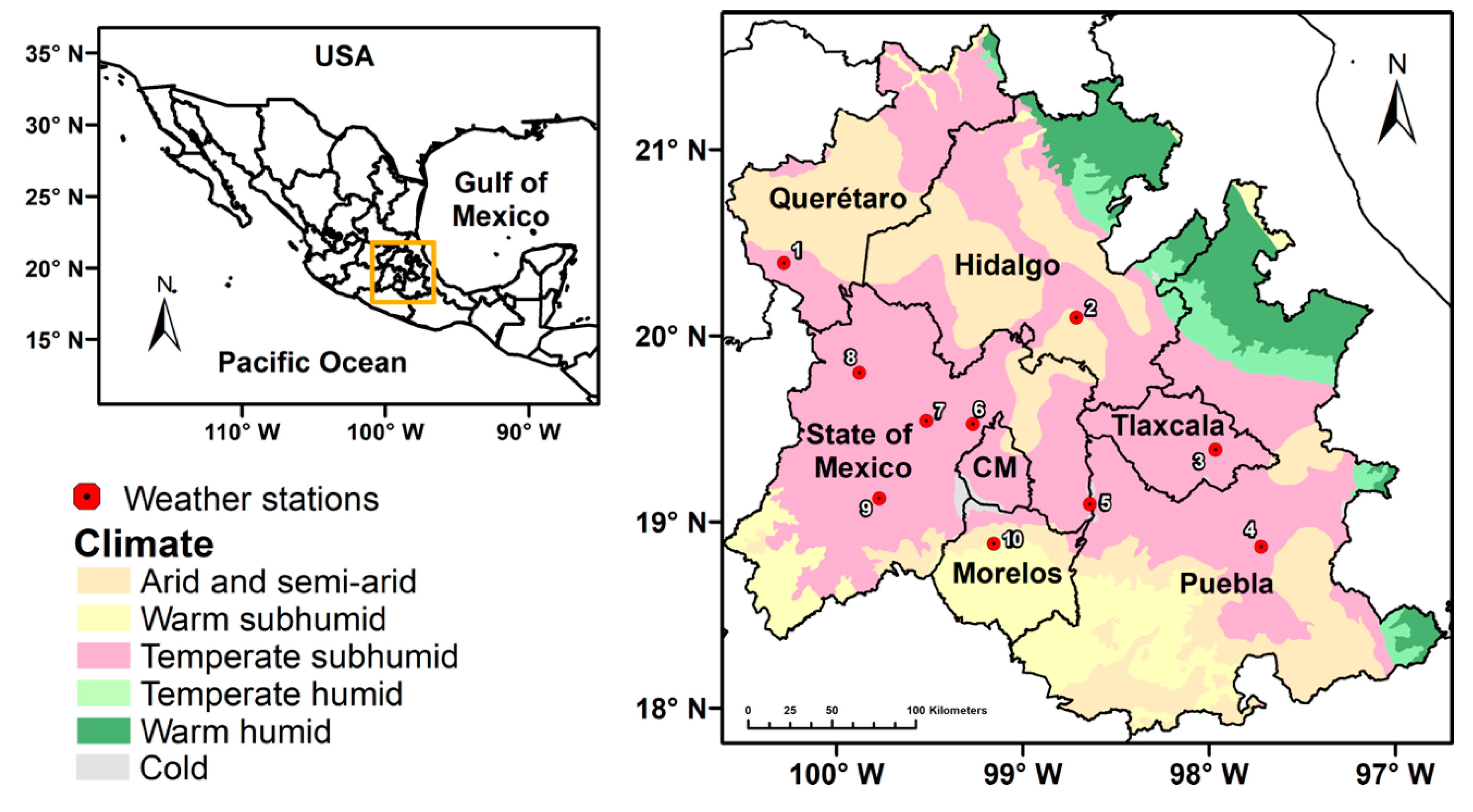
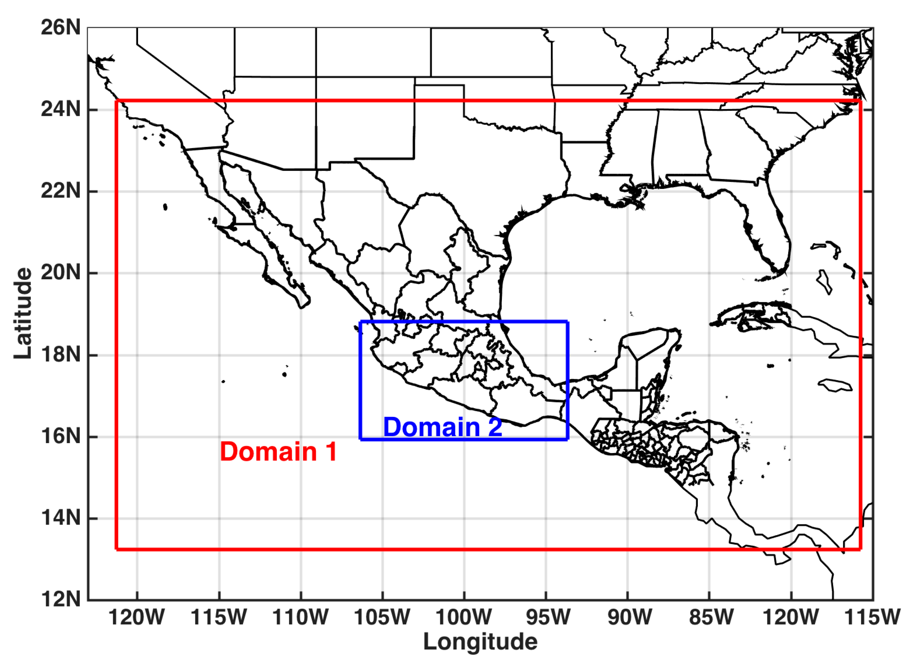
2. Study Area
3. Methods and Data
3.1. Model Configuration
3.2. Description and Assessment of the Experiments
3.3. Meteorological Data
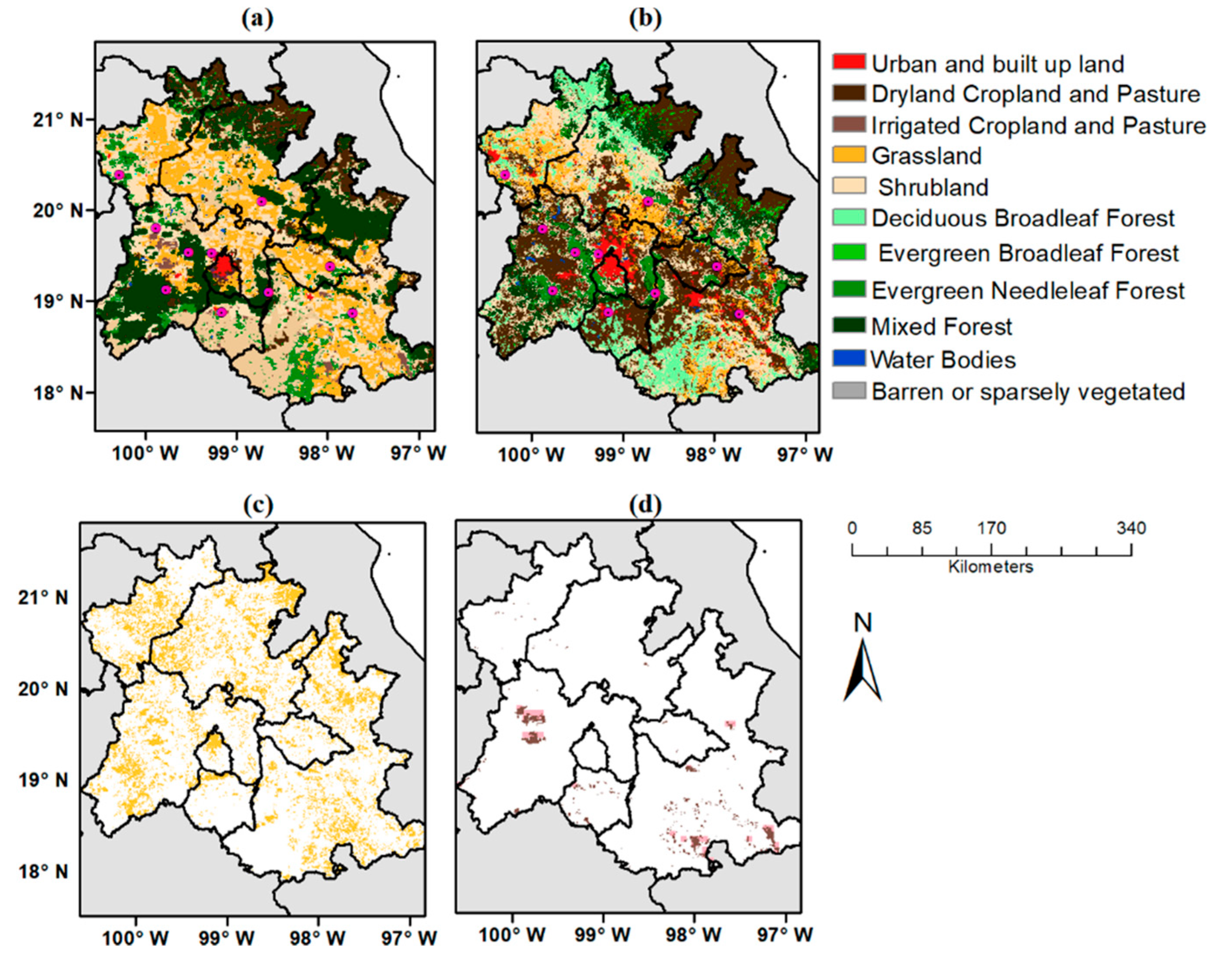
3.4. LULC Dataset
Changes of LULC
4. Results and Discussion
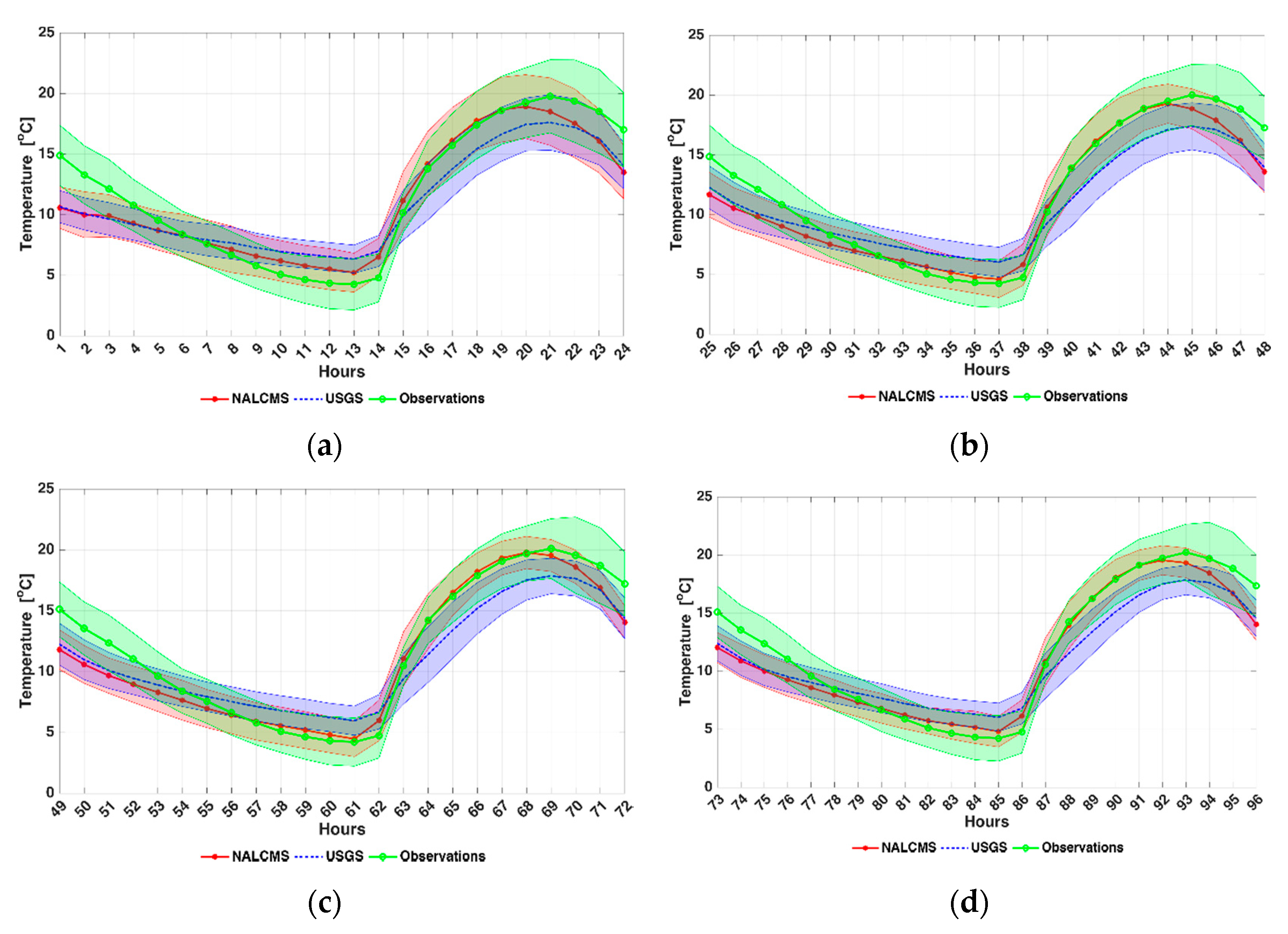
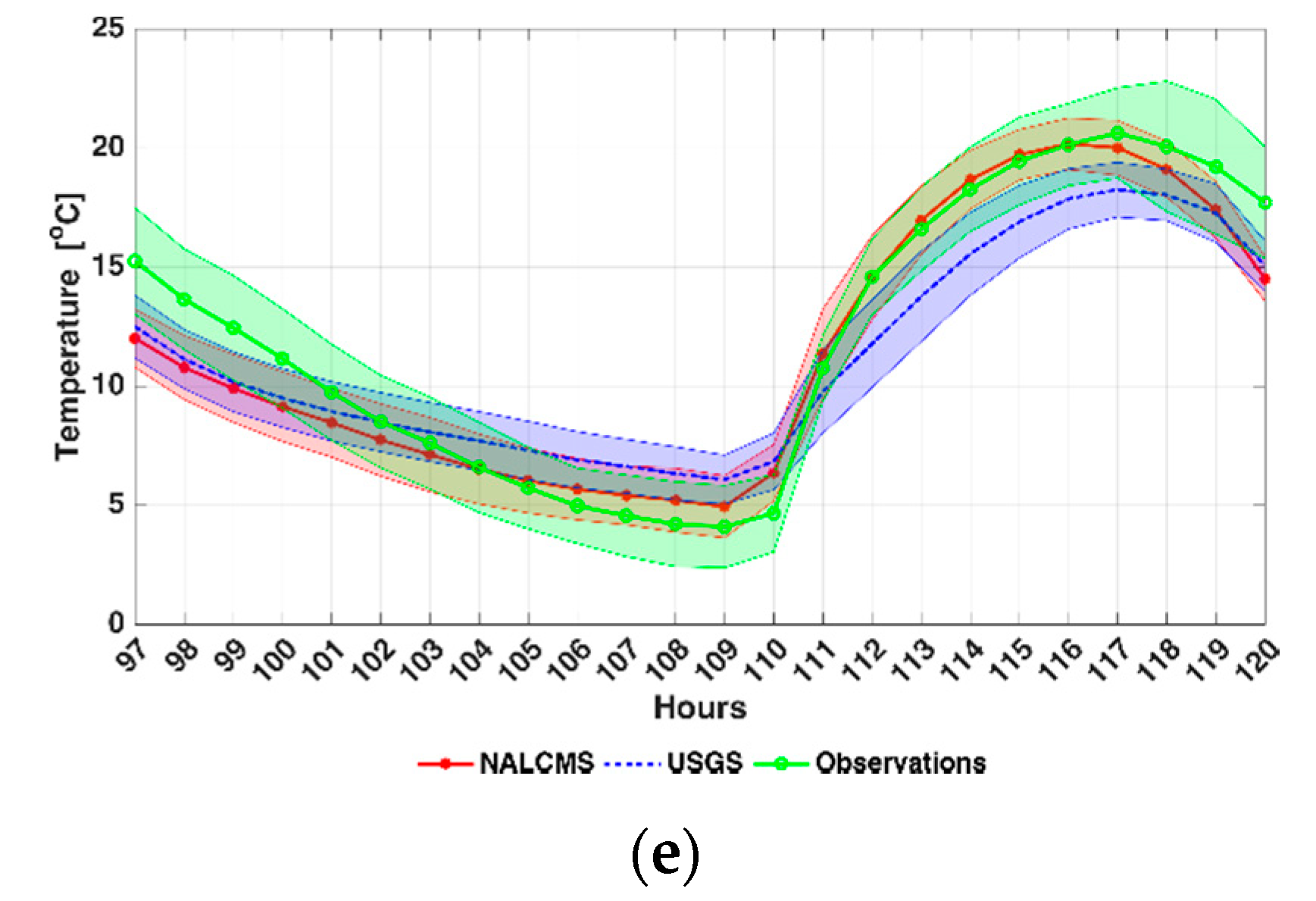
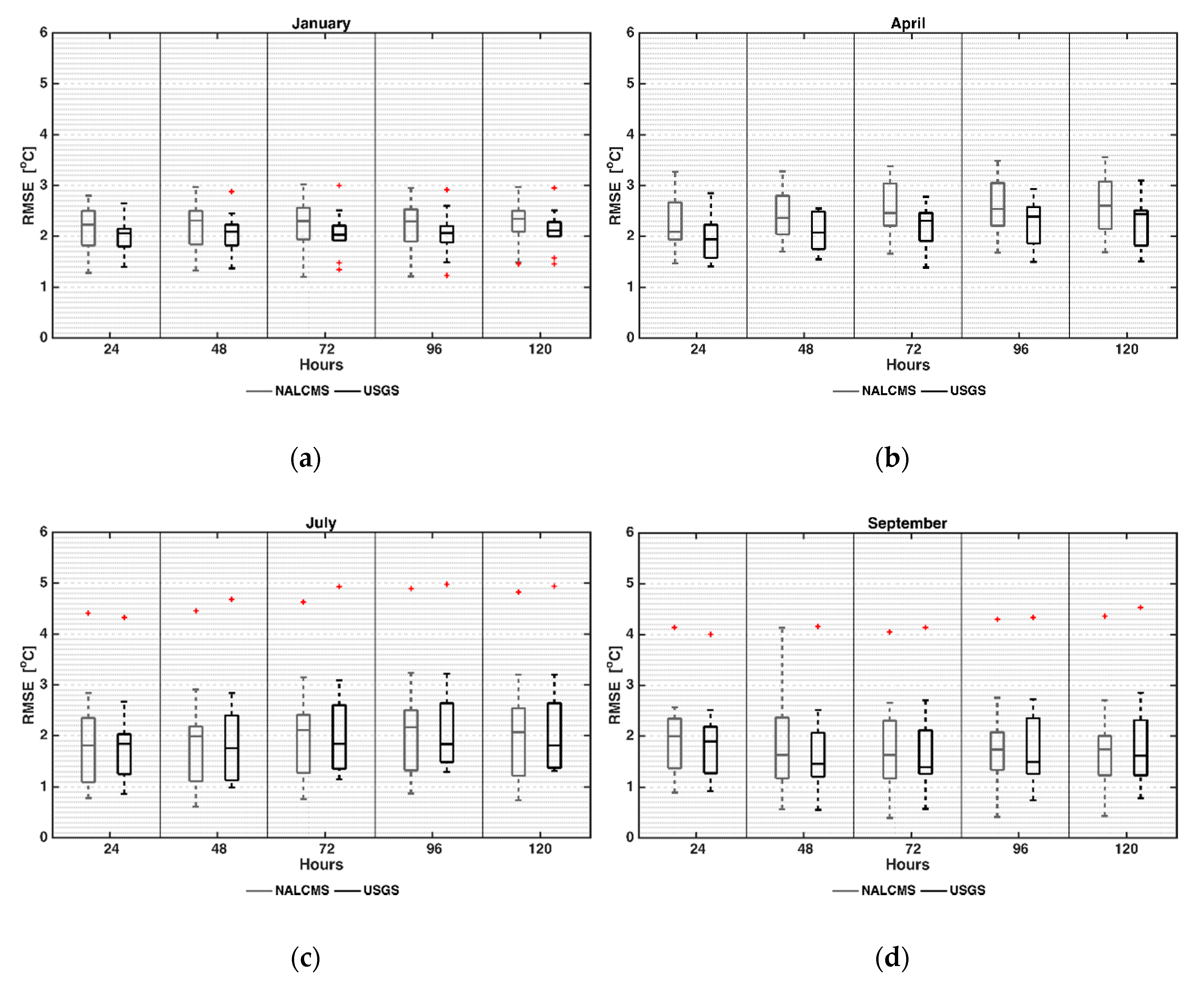
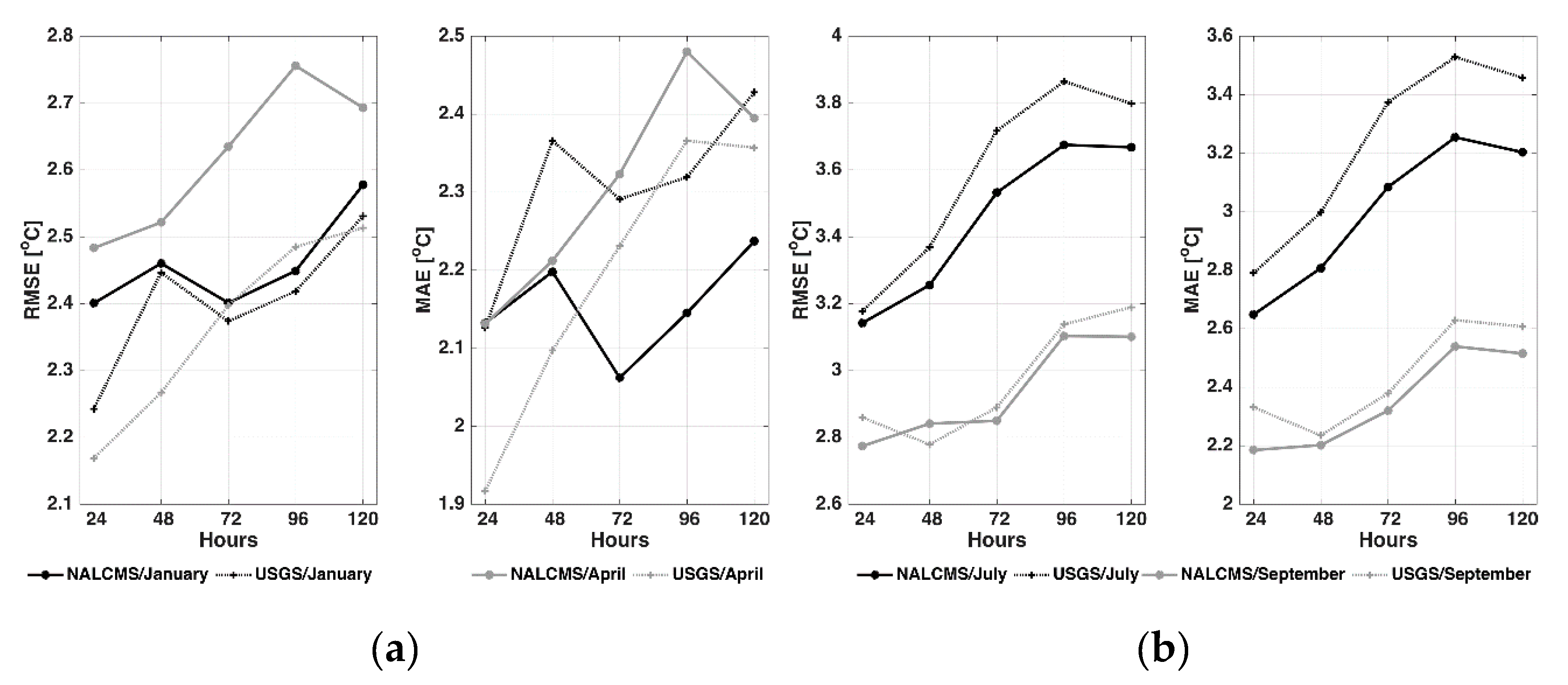
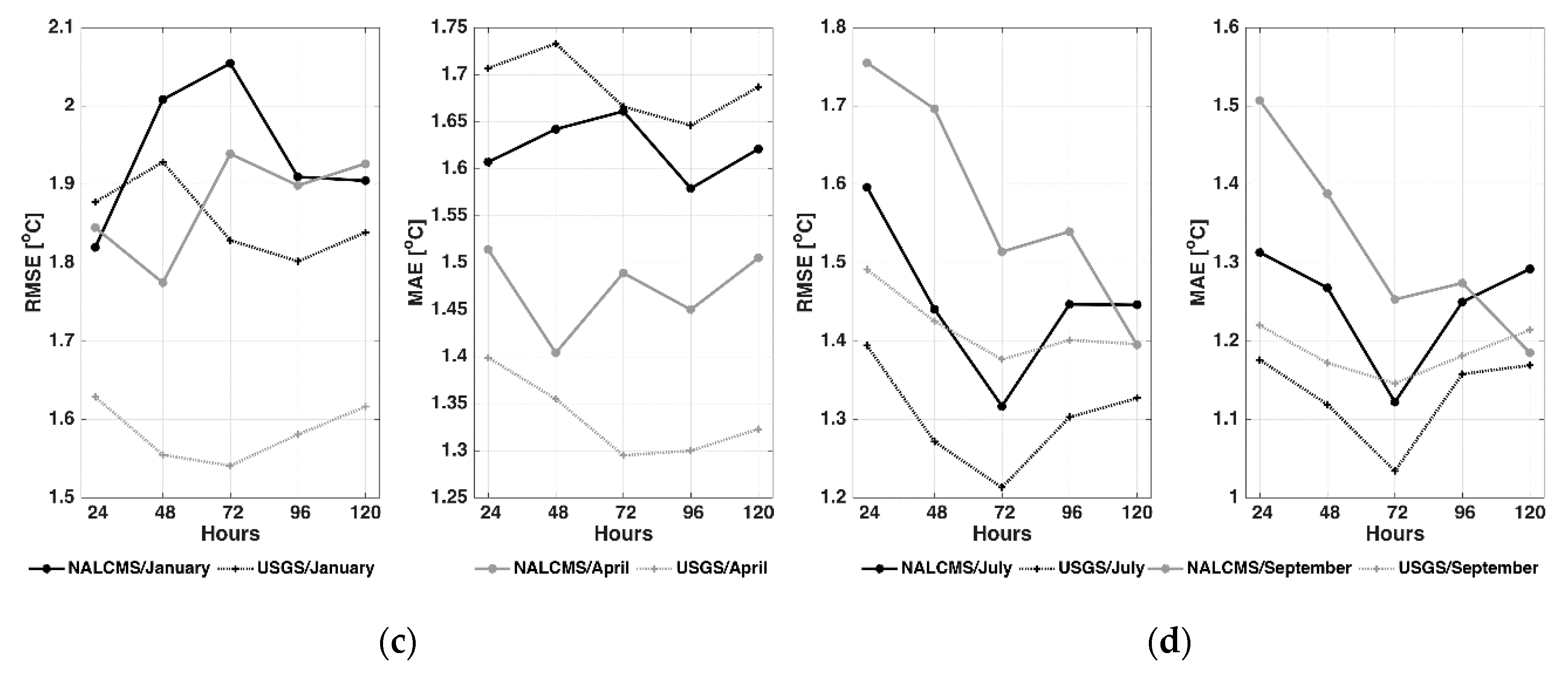
4.1. Near Surface Temperature
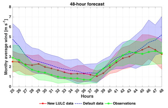
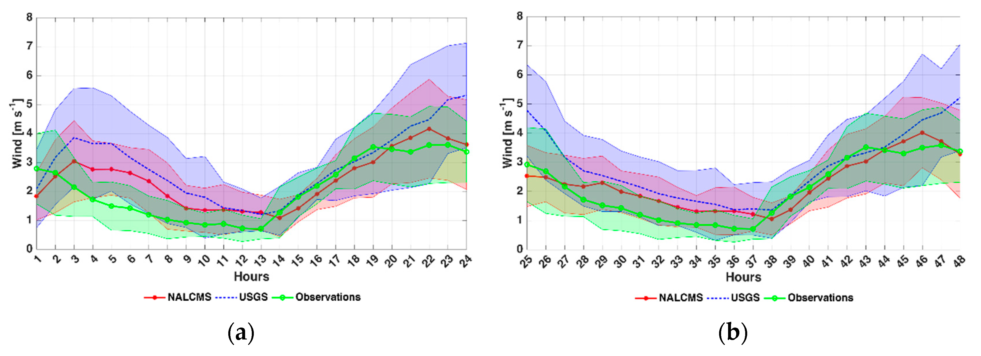
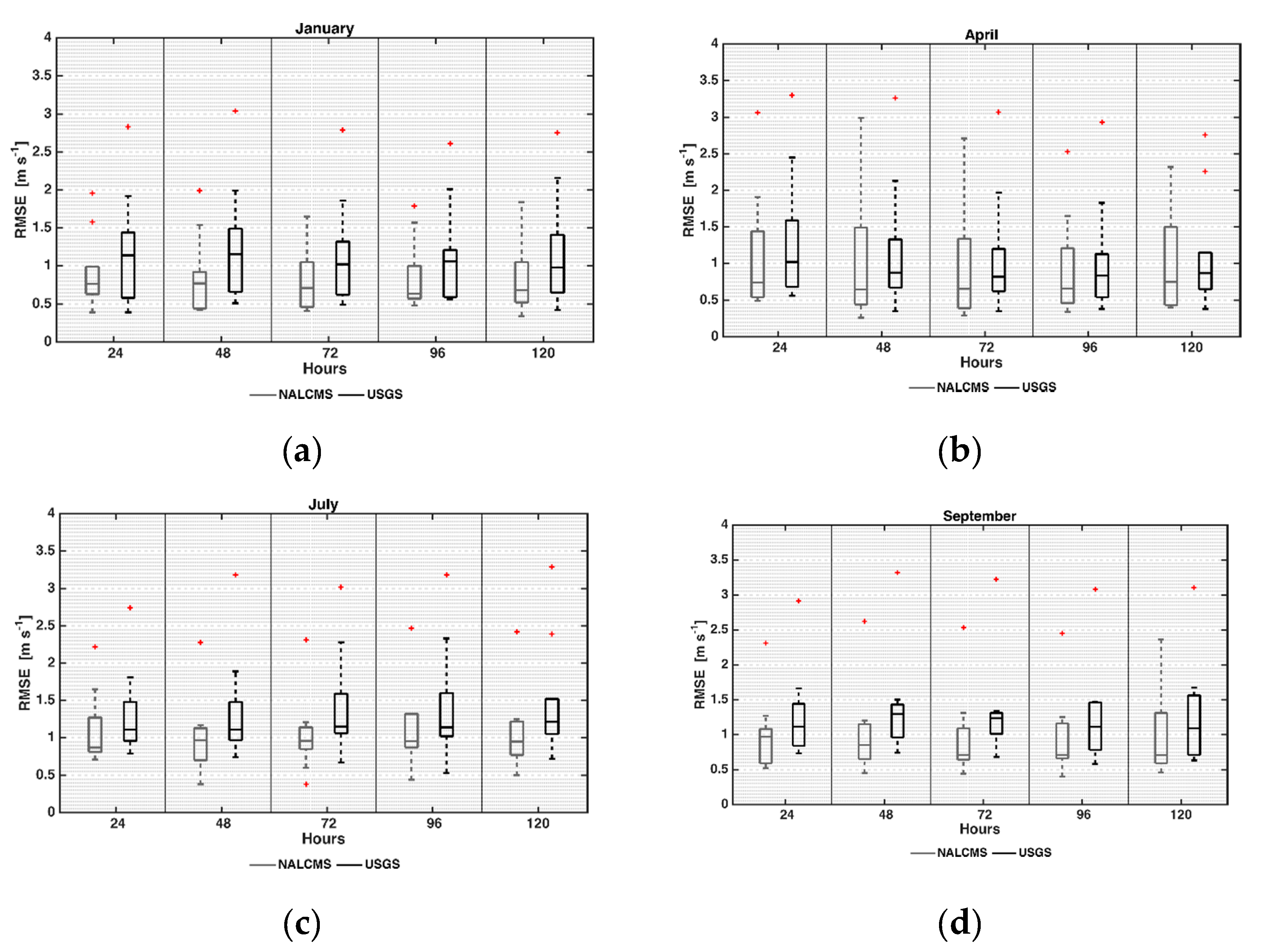
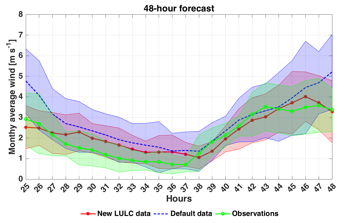
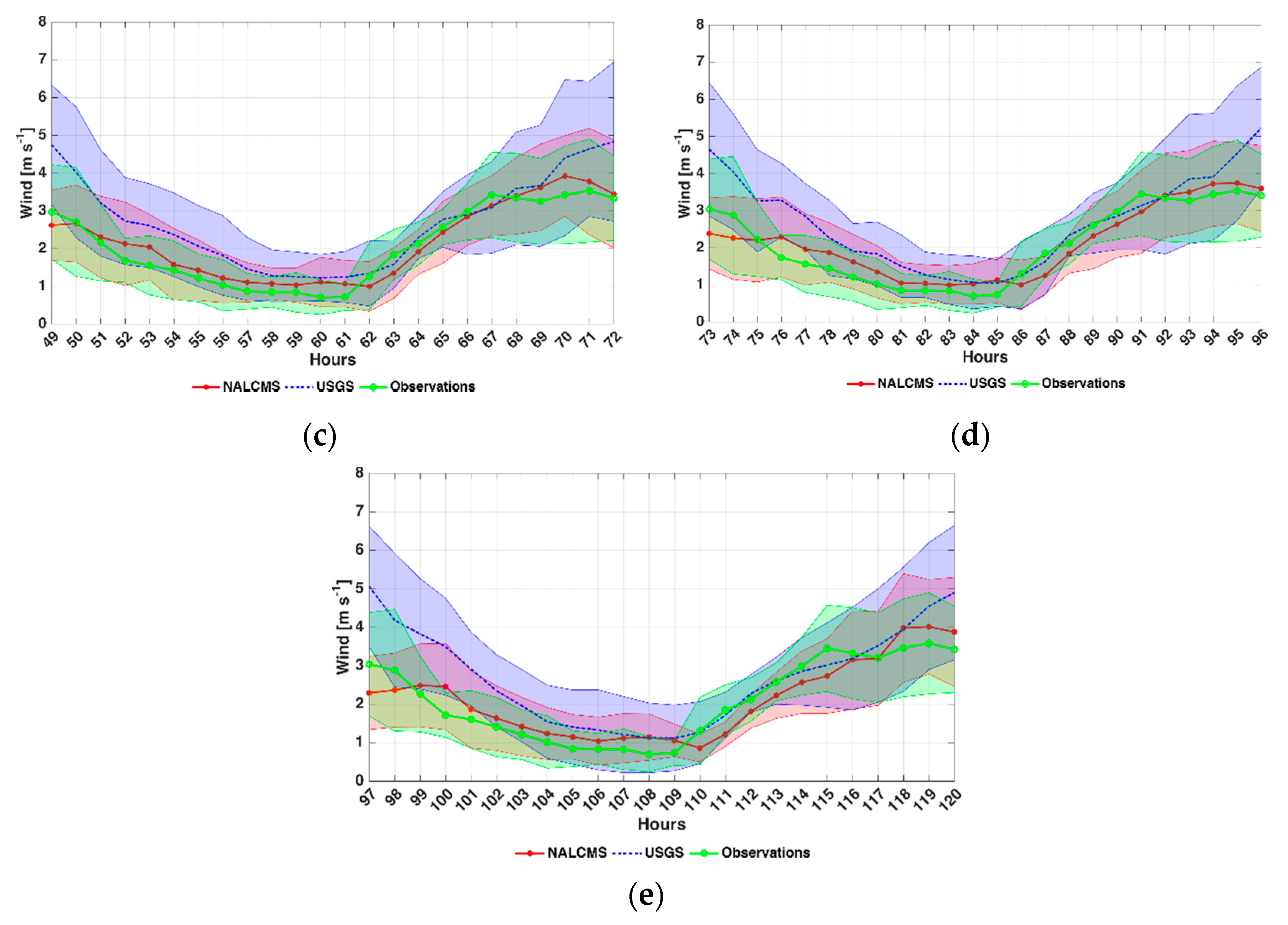
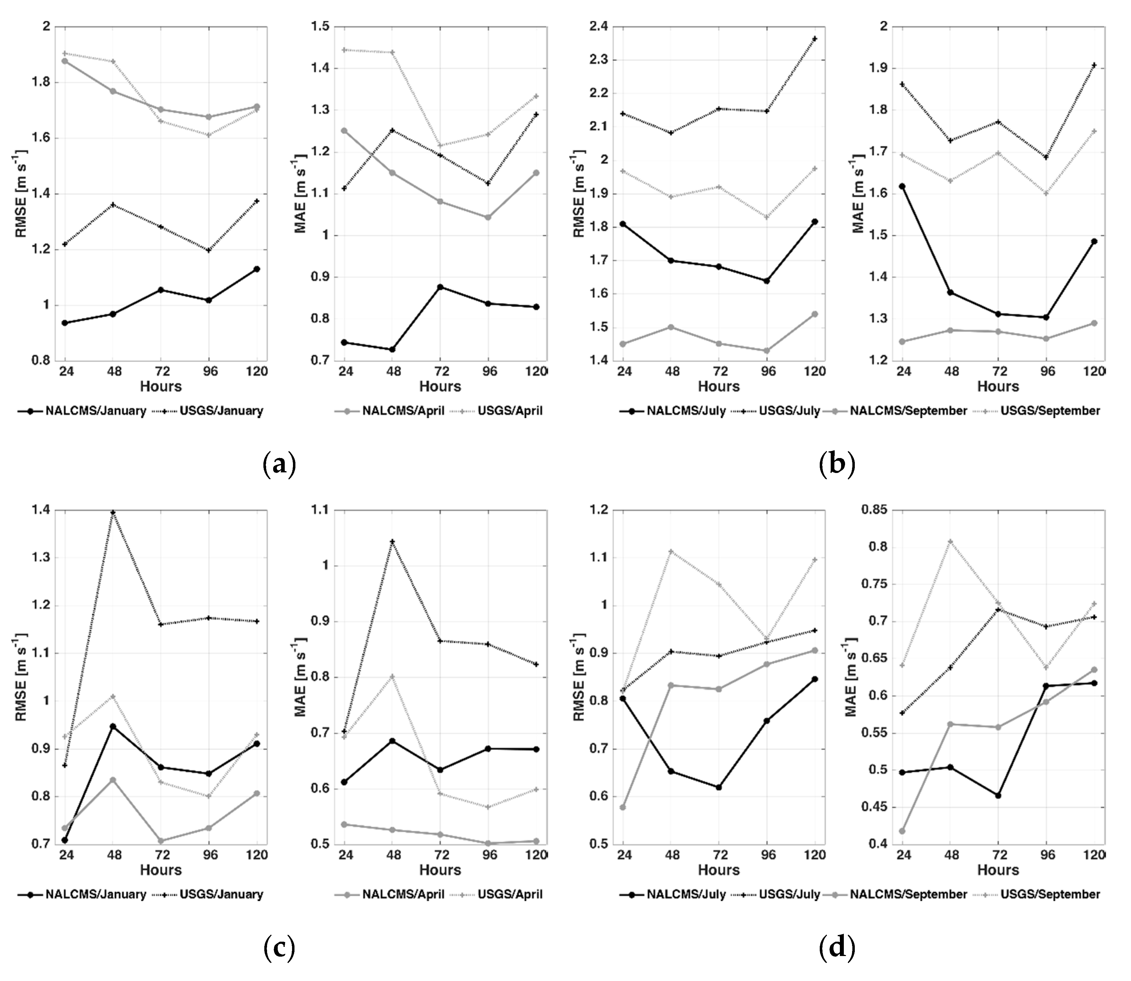
4.2. Wind Speed
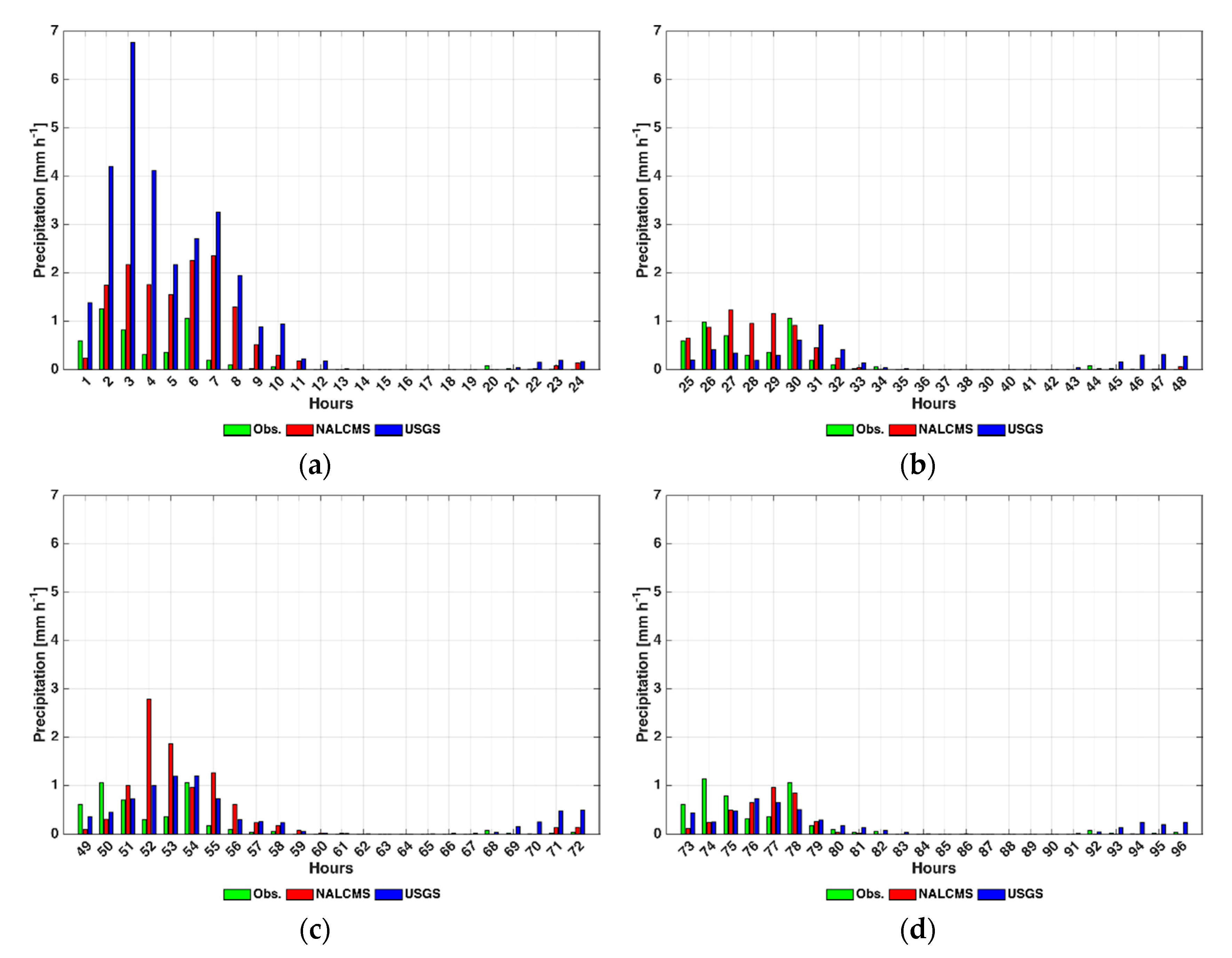
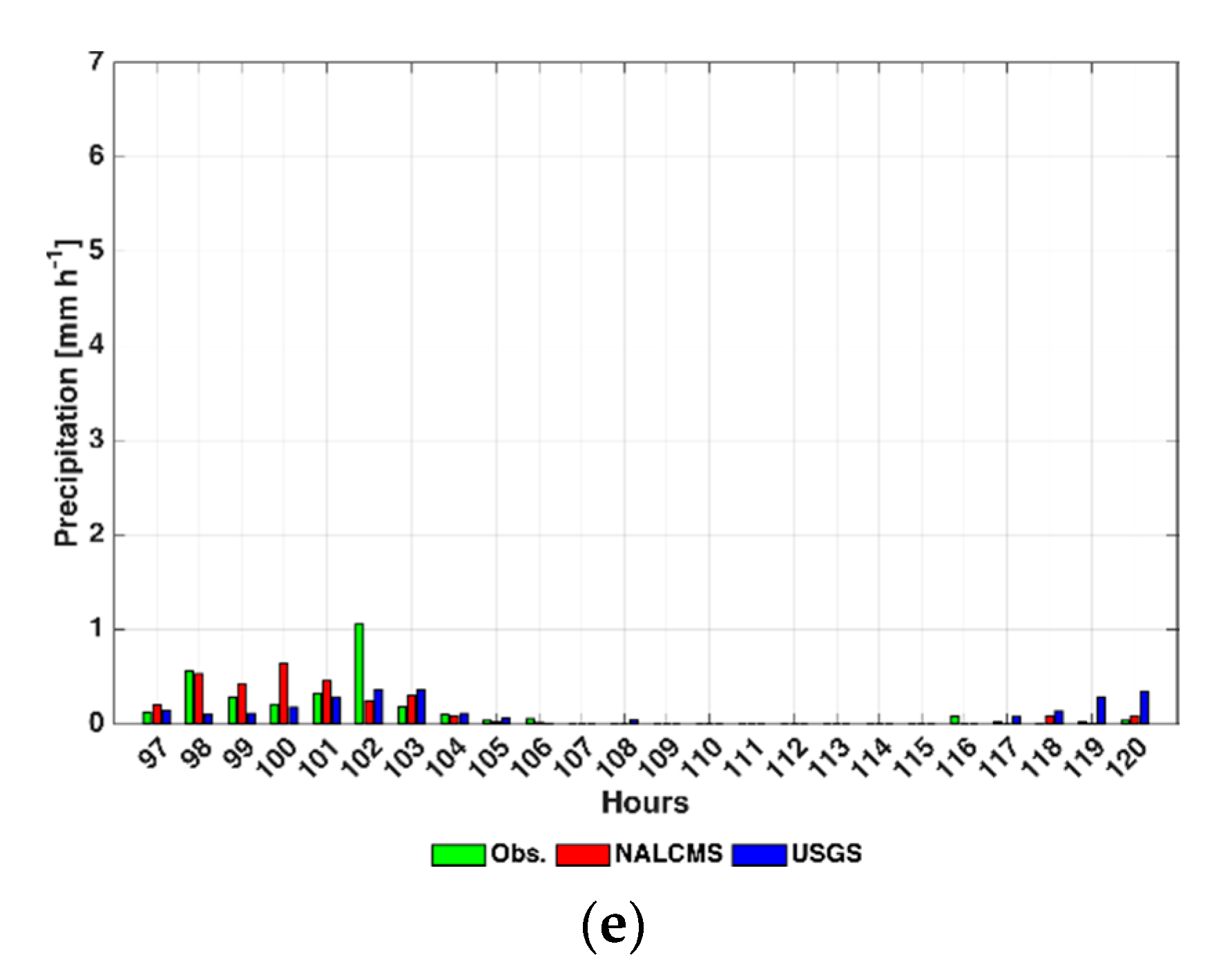
4.3. Precipitation
4.4. Physical Processes
5. Conclusions
Supplementary Materials
Author Contributions
Funding
Acknowledgments
Conflicts of Interest
References
- Grimmond, S. Urbanization and global environmental change: Local effects of urban warming. Geogr. J. 2007, 173, 83–88. [Google Scholar] [CrossRef]
- Mahmood, R.; Quintanar, A.; Conner, G.; Leeper, R.; Dobler, S.; Pielke, R.; Syktus, J. Impacts of land use/land cover change on climate and future research priorities. Bull. Am. Meteor. Soc. 2010, 91, 37e46. [Google Scholar] [CrossRef]
- Sertel, E.; Robock, A.; Ormeci, C. Impacts of land cover data quality on regional climate simulations. Int. J. Climatol. 2010, 30, 1942–1953. [Google Scholar] [CrossRef]
- Pielke, R.; Pitman, A.; Niyogi, D.; Mahmood, R.; McApline, C.; Hossain, F.; Goldewijk, K.K.; Nair, U.; Betts, R.; Fall, S.; et al. Land use/land cover changes and climate: Modeling analysis and observational evidence. Wiley Interdiscip. Rev. Clim. Chang. 2011, 2, 828–850. [Google Scholar] [CrossRef]
- Mahmood, R.; Pielke, R.; Hubbard, K.; Niyogi, D.; Dirmeyer, P.A.; McAlpine, C.; Carleton, A.M.; Hale, R.; Gameda, S.; Beltrán-Przekurat, A.; et al. Land cover changes and their biogeophysical effects on climate. Int. J. Climatol. 2014, 34, 929–953. [Google Scholar] [CrossRef] [Green Version]
- He, J.; Yu, L.; Liu, N.; Zhao, S. Impacts of uncertainty in land surface information on simulated surface temperature and precipitation over China. Int. J. Climatol. 2017, 37, 829–847. [Google Scholar] [CrossRef]
- Hale, R.; Gallo, K.; Loveland, T. Influences of specific land use/land cover conversions on climatological normals of near surface temperature. J. Geophys. Res. 2008. [Google Scholar] [CrossRef] [Green Version]
- Tao, Z.; Santanello, J.; Chin, M.; Zhou, S.; Tan, Q.; Kemp, E.; Peters-Lidard, C. Effect of land cover on atmospheric processes and air quality over the continental United States-a NASA unified WRF (NU-WRF) model study. Atmos. Chem. Phys. 2013, 13, 6207–6226. [Google Scholar] [CrossRef] [Green Version]
- Teklay, A.; Dile, Y.; Asfaw, D.; Bayabil, H.; Sisay, K. Impacts of land surface model and land use data on WRF model simulations of rainfall and temperature over Lake Tana Basin, Ethiopia. Heliyon 2019, 5, e02469. [Google Scholar] [CrossRef]
- Van Asselen, S.; Verburg, P. Land cover change or land-use intensification: Simulating land system change with a global-scale land change model. Glob. Chang. Biol. 2013, 19. [Google Scholar] [CrossRef]
- Li, J.; Zheng, X.; Zhang, C.; Chen, Y. Impact of land-use and land-cover change on meteorology in the Beijing–Tianjin–Hebei Region from 1990 to 2010. Sustainability 2018, 10, 176. [Google Scholar] [CrossRef] [Green Version]
- De Meij, A.; Vinuesa, J. Impact of SRTM and Corine Land Cover data on meteorological parameters using WRF. Atmos. Res. 2014, 143, 351–370. [Google Scholar] [CrossRef]
- Lai, A.; Liu, Y.; Chen, X.; Chang, M.; Fan, Q.; Chan, P.; Wang, X.; Dai, J. Impact of land-use change on atmospheric environment using refined land surface properties in the Pearl River Delta, China. Adv. Meteorol. 2016. [Google Scholar] [CrossRef] [Green Version]
- Kirthiga, S.; Patel, N. Impact of updating land surface data on micrometeorological weather simulations from the WRF model. Atmosfera 2018, 31, 165–183. [Google Scholar] [CrossRef] [Green Version]
- Lamptey, B.; Barron, E.; Pollard, D. Impacts of agriculture and urbanization on the climate of the Northeastern United States. Glob. Planet. Chang. 2005, 49, 203–221. [Google Scholar] [CrossRef]
- Pielke, R. Mesoscale Meteorological Modeling, 3rd ed.; Academic Press: New York, NY, USA, 2013. [Google Scholar]
- Shamsipour, A.; Azizi, G.; Ahmadabad, M.; Moghbel, M. Surface temperature pattern of asphalt, soil and grass in different weather condition. J. Biodivers. Environ. Sci. 2013, 3, 80–89. [Google Scholar]
- Chudnovsky, A.; Ben-Dor, E.; Saaroni, H. Diurnal thermal behavior of selected urban objects using remote sensing measurements. Energy Build. 2004, 36, 1063–1074. [Google Scholar] [CrossRef]
- Trusilova, K.; Jung, M.; Churkina, G.; Karsten, U.; Heimann, M.; Claussen, M. Urbanization impacts on the climate in Europe: Numerical experiments by the PSU-NCAR mesoscale model (MM5). J. Appl. Meteorol. Climatol. 2008, 47, 1442–1455. [Google Scholar] [CrossRef] [Green Version]
- Mote, T.; Lacke, M.; Shepherd, J. Radar signatures of the urban effect on precipitation distribution: A case study for Atlanta, Georgia. Geophys Res. Lett. 2007. [Google Scholar] [CrossRef]
- Lei, M.; Niyogi, D.; Kishtawa, C.; Pielke, R.; Beltrán-Przekurat, A.; Nobis, T.; Vaidya, S. Effect of explicit urban land surface representation on the simulation of the 26 July 2005 heavy rain event over Mumbai, India. Atmos. Chem. Phys. 2008, 8, 5975–5995. [Google Scholar] [CrossRef] [Green Version]
- Kishtawal, C.; Niyogi, D.; Tewari, M.; Pielke, R.; Shepherd, J. Urbanization signature in the observed heavy rainfall climatology over India. Int. J. Climatol. 2010, 30, 1908–1916. [Google Scholar] [CrossRef] [Green Version]
- Niyogi, D.; Pyle, P.; Lei, M.; Arya, S.; Kishtawal, C.; Shepherd, M.; Chen, F.; Wolfe, B. Urban modification of thunderstorms: An observational storm climatology and model case study for the Indianapolis urban region. J. Appl. Meteorol. Climatol. 2011, 50, 1129–1144. [Google Scholar] [CrossRef]
- Mitram, C.; Shepherd, J.; Jordan, T. On the relationship between the premonsoonal rainfall climatology and urban land cover dynamics in Kolkata city, India. Int. J. Climatol. 2012, 32, 1443–1454. [Google Scholar] [CrossRef]
- Mas, J.; Velázquez, A.; Díaz-Gallegos, J.; Mayorga-Saucedo, R.; Alcántara, C.; Bocco, G.; Castro, R.; Fernández, T.; Pérez-Vega, A. Assessing land use/cover changes: A nationwide multidate spatial database for Mexico. Int. J. Appl. Earth Obs. 2004, 5, 249–261. [Google Scholar] [CrossRef]
- Jáuregui, E. Effects of revegetation and new artificial water bodies on the climate of northeast Mexico City. Energy Build. 1990, 15, 447–455. [Google Scholar] [CrossRef]
- Jáuregui, E.; Romales, E. Urban effects on convective precipitation in Mexico City. Atmos. Environ. 1996, 30, 3383–3389. [Google Scholar] [CrossRef]
- Jazcilevich, A.; Fuentes, V.; Jáuregui, E.; Luna, E. Simulated urban climate response to historical land use modification in the basin of Mexico. Clim. Chang. 2000, 44, 515–536. [Google Scholar] [CrossRef]
- López-Espinoza, E.; Zavala-Hidalgo, J.; Gómez-Ramos, O. Weather forecast sensitivity to changes in urban land covers using the WRF model for central Mexico. Atmosfera 2012, 25, 127–154. [Google Scholar]
- Ochoa, C.; Quintanar, A.; Raga, G.; Baumgardner, D. Changes in intense precipitation events in Mexico City. J. Hydrometeorol. 2015, 16, 1804–1820. [Google Scholar] [CrossRef]
- López-Bravo, C.; Caetano, E.; Magaña, V. Forecasting summertime surface temperature and precipitation in the Mexico City metropolitan area: Sensitivity of the WRF model to land cover changes. Front. Earth Sci. 2018. [Google Scholar] [CrossRef] [Green Version]
- Lozano-García, M.; Ortega-Guerrero, B.; Caballero-Miranda, M.; Urrutia-Fucugauchi, J. Late Pleistocene and Holocene paleoenvironments of Chalco lake, central Mexico. Quat. Res. 1993, 40, 332–342. [Google Scholar] [CrossRef]
- Loveland, T.; Reed, B.; Brown, J.; Ohlen, D.; Zhu, Z.; Yang, L.; Merchant, J. Development of a global land cover characteristics database and IGBP DISCover from 1 km AVHRR data. Int. J. Remote Sens. 2000, 21, 1303–1330. [Google Scholar] [CrossRef]
- Colditz, R.; López-Saldaña, G.; Maeda, P.; Argumedo-Espinoza, J.; Meneses-Tovar, C.; Victoria-Hérnandez, A.; Zermeño-Benítez, C.; Cruz-López, I.; Ressl, R. Generation and analysis of the 2005 land cover map for Mexico using 250m MODIS data. Remote Sens. Environ. 2012, 123, 541–552. [Google Scholar] [CrossRef]
- Kain, J. The Kain–Fritsch convective parameterization: An update. J. Appl. Meteorol. 2004, 43, 170–181. [Google Scholar] [CrossRef] [Green Version]
- A Description of the Advanced Research WRF Version 3. NCAR Technical Note NCAR/TN-475+STR. National Center for Atmospheric Research. Available online: https://doi:10.5065/D68S4MVH (accessed on 3 September 2020).
- A Multi-Layer Soil Temperature Model for MM5. Available online: https://www.researchgate.net/publication/259865197_A_Multilayer_Soil_Temperature_Model_for_MM5 (accessed on 3 September 2020).
- Zeng, X.; Wang, N.; Wang, Y.; Zheng, Y.; Zhou, Z.; Wang, G.; Chen, C.; Liu, H. WRF-simulated sensitivity to land surface schemes in short and medium ranges for a high-temperature event in East China: A comparative study. J. Adv. Model Earth Syst. 2015, 7, 1305–1325. [Google Scholar] [CrossRef]
- Lee, C.; Kim, J.; Belorid, M.; Zhao, P. Performance evaluation of four different land surface models in WRF. Asian J. Atmos. Environ. 2016, 10, 42–50. [Google Scholar] [CrossRef] [Green Version]
- Jain, S.; Panda, J.; Rath, S.; Devara, P. Evaluating land surface models in WRF simulations over DMIC region. Indian J. Sci. Technol. 2017, 10, 1–24. [Google Scholar] [CrossRef]
- Wilks, D. Statistical Methods in the Atmospheric Sciences, 3rd ed.; Academic Press: San Diego, CA, USA, 2011. [Google Scholar]
- American Geophysical Union. Comparison and Evaluation of Five Global Land Cover Datasets for Mexico. Spring Meeting 2013 Abstract Id. A23A-02. Available online: https://ui.adsabs.harvard.edu/abs/2013AGUSM.A23A..02L/abstract (accessed on 3 September 2020).
- Yang, H.; Li, S.; Chen, J.; Zhang, X.; Xu, S. The standardization and harmonization of land cover classification systems towards harmonized datasets: A review. ISPRS Int. J. Geo-Inf. 2017, 6, 154. [Google Scholar] [CrossRef] [Green Version]
- Colditz, R.; Llamas, R.; Ressl, R. Detecting Change Areas in Mexico Between 2005 and 2010 Using 250 m MODIS Images. IEEE J. Select Top Appl. Earth Obs. Remote Sens. 2014, 7, 3358–3372. [Google Scholar] [CrossRef]
- Barrales-Hassan, R. Impacto del Cambio de Uso de Suelo y Cobertura Vegetal en el Pronóstico Numérico del Tiempo. Bachelor’s Thesis, Universidad Nacional Autónoma de México, Mexico City, Mexico, 2017. [Google Scholar]
- A Land Use and Land Cover Classification System for Use with Remote Sensor Data. 1st ed. United States Geological Survey. Available online: https://pubs.usgs.gov/pp/0964/report.pdf (accessed on 3 September 2020).
- Bai, L. Comparison and Validation of Five Land Cover Products over the AFRICAN Continent; Lund University: Lund, Sweden, 2010. [Google Scholar]
- Latifovic, R.; Zhu, Z.; Cihlar, J.; Giri, C.; Olthof, I. Land cover mapping of North and Central America-global land cover 2000. Remote Sens. Environ. 2004, 89, 116–127. [Google Scholar] [CrossRef]
- McCallum, I.; Obersteiner, M.; Nilsson, S.; Shvidenko, A. A spatial comparison of four satellite derived 1 km global land cover datasets. Int. J. Appl. Earth Obs. 2006, 8, 246–255. [Google Scholar] [CrossRef]
- Zhou, L.; Dickinson, R.; Tian, Y.; Fang, J.; Li, Q.; Kaufmann, R.; Tucker, C.; Myneni, R. Evidence for a significant urbanization effect on climate in China. Proc. Natl. Acad. Sci. USA 2004, 101, 9540–9544. [Google Scholar] [CrossRef] [PubMed] [Green Version]
- Jin, J.; Miller, N.; Schlegel, N. Sensitivity study of four land surface schemes in the WRF model. Adv. Meteorol. 2010. [Google Scholar] [CrossRef] [Green Version]


| USGS | NALCMS | |
|---|---|---|
| Sensor | AVHRR | MODIS |
| Period of data collection | April 1992–March 1993 | January 2005–December 2005 |
| Processing | By continent | 3 regions |
| Input data | Monthly NDVI compositions | Different data by country |
| Spatial resolution | 1 km | 250 m |
| Classification strategy | Unsupervised based on grouping | Supervised with threes C5 (for Mexico) |
| Legend system | 24 USGS | 19 LCCS-FAO |
| Developers | USGS-IGBP | CCRS, USGS, INEGI, CONABIO, CONAFOR |
| Anderson’s Classification Scheme | USGS | NALCMS |
|---|---|---|
| Urban | Urban and built up land | Urban and built-up |
| Agricultural land | Dryland cropland/pasture | Cropland |
| Irrigated cropland/pasture | ||
| Rangeland | Grassland | Tropical or sub-tropical grassland |
| Temperate or sub-polar grassland | ||
| Shrubland | Tropical or sub-tropical shrubland | |
| Temperate or sub-polar shrubland | ||
| Forest | Deciduous broadleaf forest | Tropical or sub-tropical broadleaf deciduous forest |
| Temperate or sub-polar broadleaf deciduous forest | ||
| Evergreen broadleaf forest | Tropical or sub-tropical broadleaf evergreen forest | |
| Evergreen needleleaf forest | Temperate or sub-polar needleleaf evergreen forest | |
| Mixed forest | Mixed forest | |
| Water | Water bodies | Water |
| Barren land | Barren or sparsely vegetated | Barren land |
| ID | Station | USGS | NALCMS |
|---|---|---|---|
| 1 | Huimilpan, Qro. | Shrubland | Cropland |
| 2 | Pachuca, Hgo. | Grassland | Grassland |
| 3 | Huamantla, Tlax. | Evergreen Needleleaf Forest | Cropland |
| 4 | Universidad Tecnológica de Tecamachalco, Pue. | Evergreen Needleleaf Forest | Cropland |
| 5 | Parque-Izta-Popo, Edo. Méx. | Mixed Forest | Evergreen Needleleaf Forest |
| 6 | Presa Madín, Edo. Méx. | Shrubland | Urban and Built-Up Land |
| 7 | Cerro Catedral, Edo. Méx. | Shrubland | Evergreen Needleleaf Forest |
| 8 | Atlacomulco, Edo. Méx. | Shrubland | Cropland |
| 9 | Nevado de Toluca, Edo. Méx. | Mixed Forest | Evergreen Needleleaf Forest |
| 10 | Instituto Mexicano de Tecnología del Agua, Mor. | Shrubland | Cropland |
| Land Cover Category | Albedo (%) [ALBEDO] | Roughness Length (m) [SFZ0] | Emissivity (% at 9 µ m) [SFEM] | |||
|---|---|---|---|---|---|---|
| Sum | Win | Sum | Win | Sum | Win | |
| Urban and Built-Up Land | 15 | 15 | 0.80 | 0.80 | 88 | 88 |
| Dryland Cropland and Pasture | 17 | 23 | 0.15 | 0.05 | 98.5 | 92 |
| Irrigated Cropland and Pasture | 18 | 23 | 0.15 | 0.05 | 98.5 | 92 |
| Grassland | 19 | 23 | 0.12 | 0.10 | 98.5 | 92 |
| Shrubland | 22 | 25 | 0.10 | 0.10 | 88 | 88 |
| Evergreen Needleleaf Forest | 12 | 12 | 0.50 | 0.50 | 95 | 95 |
| Mixed Forest | 13 | 14 | 0.50 | 0.50 | 94 | 94 |
| Hourly Precipitation [mm h−1] | ||||||
|---|---|---|---|---|---|---|
| 24-h | 48-h | 72-h | 96-h | 120-h | ||
| July | NALCMS | <1.13 | <1.24 | <1.04 | <0.96 | <0.73 |
| USGS | <0.78 | <0.60 | <1.15 | <0.59 | <0.38 | |
| September | NALCMS | <1.42 | <1.35 | <1.56 | <0.77 | <1.11 |
| USGS | <0.77 | <0.41 | <0.52 | <0.79 | <0.84 | |
Publisher’s Note: MDPI stays neutral with regard to jurisdictional claims in published maps and institutional affiliations. |
© 2020 by the authors. Licensee MDPI, Basel, Switzerland. This article is an open access article distributed under the terms and conditions of the Creative Commons Attribution (CC BY) license (http://creativecommons.org/licenses/by/4.0/).
Share and Cite
López-Espinoza, E.D.; Zavala-Hidalgo, J.; Mahmood, R.; Gómez-Ramos, O. Assessing the Impact of Land Use and Land Cover Data Representation on Weather Forecast Quality: A Case Study in Central Mexico. Atmosphere 2020, 11, 1242. https://doi.org/10.3390/atmos11111242
López-Espinoza ED, Zavala-Hidalgo J, Mahmood R, Gómez-Ramos O. Assessing the Impact of Land Use and Land Cover Data Representation on Weather Forecast Quality: A Case Study in Central Mexico. Atmosphere. 2020; 11(11):1242. https://doi.org/10.3390/atmos11111242
Chicago/Turabian StyleLópez-Espinoza, Erika Danaé, Jorge Zavala-Hidalgo, Rezaul Mahmood, and Octavio Gómez-Ramos. 2020. "Assessing the Impact of Land Use and Land Cover Data Representation on Weather Forecast Quality: A Case Study in Central Mexico" Atmosphere 11, no. 11: 1242. https://doi.org/10.3390/atmos11111242
APA StyleLópez-Espinoza, E. D., Zavala-Hidalgo, J., Mahmood, R., & Gómez-Ramos, O. (2020). Assessing the Impact of Land Use and Land Cover Data Representation on Weather Forecast Quality: A Case Study in Central Mexico. Atmosphere, 11(11), 1242. https://doi.org/10.3390/atmos11111242