Site Suitability Analysis for Low Cost Sensor Networks for Urban Spatially Dense Air Pollution Monitoring

Abstract

Urban air pollution continues to represent a primary concern for human health, despite significant efforts by public authorities for mitigating its effects. Regulatory monitoring networks are essential tools for air pollution monitoring. However, they are sparse networks, unable to capture the spatial variability of the air pollutants. For addressing this issue, networks of low cost stations are deployed, supplementing the regulatory stations. Regarding this application, an important question is where these stations are installed The objective of this study was to generate a site suitability map for the development of a network of low cost multi-sensor stations across a city for a spatially dense urban air quality monitoring. To do that, a site suitability analysis was developed based on two geographical variables properly selected for representing the impact of urban pollutant sources and urban form on the pollutant concentrations. By processing information about emissions patterns and street canyon effects, we were able to identify air quality hotspot areas supposed to show high spatial variability. Low cost monitoring stations, there located, are able to provide that informative content, which is lacking for both regulatory monitoring networks and predictive modelling for high resolution air quality mapping.

1. Introduction

Despite continuous and significant efforts by public authorities, air quality continues to represent a primary concern for human health at global scale. An evidence of air quality pollution burden was recently provided by the effects of lockdowns due to SARS-CoV-2 pandemic: the restriction imposed to most of the human activities determined a significant drop of air pollution levels [1]. Apart from well-established causality links with severe and chronic respiratory issues and cancer, researchers have recently hypothesized a correlation link with viruses spreading including SARS-CoV-2, in particular by particulate matter at relatively high concentrations. As such, air quality monitoring is paramount for environmental and health management and is currently regulated by extensive and precise legal frameworks [2,3]. Usually these frameworks rely on costly and cumbersome monitoring stations, including multiple bench top analyzers, which require frequent maintenance and recalibration procedure. These conditions almost everywhere caused the deployment of sparse network of regulatory grade analyzers, which are unable to cope with perceived and measured high spatial and temporal variation of the concentration of pollutants.

Over last decades, public authorities have increasingly adopted an integrated approach for air quality management that includes direct measurements and modelling of pollutant concentrations. While the direct measurements provide direct information of the air pollution level at given positions, pollutant dispersion models provide an exhaustive picture of the distribution of air pollution throughout urban areas. Pollutant concentrations have always been measured by sparsely distributed regulatory monitoring networks. Recently, with the increasing availability of low-cost sensors, their data quality is still debated [4], deployments of these sensors have been used for supplementing regulatory monitors and provide spatially-resolved air pollutant concentration fields. Indeed, such applications intend to resolve the critical problem to better characterize the spatial variations of air urban pollution. The further advantage of using these networks is to obtain a finer spatiotemporal granularity of measurements with lighter installation and operational costs.

Several studies [5,6,7] have shown that air pollutant concentrations have fine-scale spatial variations that are not captured by the regulatory monitors. Recently, Hugh Z. Li et al. (2019) [8] have experimented, by deploying both stationary and mobile platforms in the city of Pittsburgh, that NO₂ exhibited within-neighborhood spatial variations, with hotspots elevated by up to a factor of five above the regional background. Similarly, they observed that the within-neighborhood spatial differences in ultrafine particles could be a factor of 2.4 times regional background. Miskell et al. (2019) [9] demonstrated that very large variations in ozone concentration took place on short time- and distance scales across the city. At this scope a large number of ozone low-cost sensors was deployed in the city of Los Angeles.

Thus, using networks of low costs sensors (mobile and stationary) within a city, neighborhood-level differences as well as pollutant spatial differences near specific sources (e.g., roadways) can be resolved and pollutant spatial variations at fine (sub-km) length scales can be quantified. Including these networks, simulation models can operate until street scale (100 m), providing more reliable predictions of the air pollutants distribution across the city. Their performance can be evaluated by comparison of simulation results to both reference network measurements, typically using regulatory monitors located in the urban background, and measurements of the low-cost sensors deployed in locations properly selected, at high spatial densities on the entire urban area.

However, important questions relevant to the deployment of networks of low-cost sensors at urban level are still to be addressed, such as the reliability of the data from low cost devices given the minimum physical intervention, or site visits aimed at minimizing the costs. Other question concerns the spatial representativeness of the monitoring locations, varying with modifiable factors as land use and emissions, and its impact on the ability of pollutant dispersion models to predict concentration fields. Another one is related to the “optimal sampling design” which means that, referred to the networks of low cost sensors, a limited number of “suitable” sites are designed for a spatially dense air pollution monitoring on the basis of which more reliable air quality forecasts across the city can be obtained as well as population pollutant exposures can be evaluated more accurately.

The deployment issue of low-cost sensor networks was addressed extensively in literature where several mathematical models, multi-objectives optimization algorithms, and near-optimal heuristics were proposed [10,11,12].

Regarding low cost air quality sensor networks, the optimization methods proposed were essentially based on several integer linear programming formulations (ILP) [12]. Optimal positions of sensors were defined while assuring air pollution coverage and minimizing total metering cost. Boubrima et al. (2019) [13] proposed an advanced ILP formulation based on simulated air pollution data clustering and modelling of coverage and connectivity by the flow concept.

Another method widely applied in literature for allocating optimal sites is a multi-criteria assessment (MCA). MCA method is often joined with geographical information systems (GIS) and it is becoming a powerful tool to resolve site suitability problems [14,15]. In their study, Alsahli and Al Harbi (2018) [14] used a GIS–MCA to combine a set of relevant geographical variables (i.e., population, wind direction, and spatial proximity to roads, industries, and high-traffic areas) for allocating optimal sites for air quality monitoring stations.

In this research work, the objective was to allocate optimal sites of stationary low-cost multi-sensor stations across a city for a spatially dense monitoring of air quality. At this scope, a spatially explicit approach based on suitability analysis was proposed. Geographical variables and location constraints were selected for representing the impact of the urban pollutant sources such as the vehicular traffic and of the urban form as the street canyon effects on the pollutant concentrations. Thus, they were combined through a spatial multi criteria evaluation, generating site suitability maps for deploying low cost multi-sensor stations for monitoring air pollution across the city, and quantifying the local spatial variability of air pollutants.

The proposed approach was applied at the case study of the City of Portici (Italy). A site suitability map of low-cost multi-sensor traffic-orientated stations was generated for monitoring NOx and PM2.5 concentrations across the city. A network of seven stations was installed on a subset of defined suitable sites, properly selected for meeting cost and installation constraints. This network intended to address the challenging objectives of the funded European Project AIR-HERITAGE under the UIA (Urban Innovative Actions) call on Air Quality.

This Project aims to enable the development of participated and fact based air quality amelioration policies by urban authorities, leveraging on enhanced and easy to communicate information about air quality for all the relevant stakeholders. High resolution information on air quality are obtained by an integrated hybrid network of fixed and mobile low-cost air quality monitors and advanced atmospheric urban pollutant dispersion models.

2. Material and Methods

The objective of this study was to generate a site suitability map for the development of a network of low-cost multi-sensor traffic-orientated stations across a city aimed at a spatially dense urban air quality monitoring. To do that, a spatial analysis approach based on GIS-multi-criteria assessment was developed and applied to the city of Portici.

In this context, the suitability was defined as the quantification of the appropriateness of candidate locations to deploy a network of low cost sensors for capturing the local spatial variability of the air pollutants within the city and it was determined on the basis of geographical variables and location constraints. On the basis of the available datasets, the street canyon effects and the traffic-related emissions were selected as geographical variables intending to represent the impact of local sources and land use on measured pollutant concentrations. In fact, street canyon effects, generated by the ratio between the buildings height and the streets width, can modify concentration patterns near roadways. Traffic-related emissions contribute to background pollutant concentrations but they are also the principal source of local variation in the concentrations of urban air pollutants. We expect higher pollutant concentrations in high traffic emissions areas [16,17].

So, traffic emissions related to NOx and PM2.5 pollutants across the city were computed by simulating traffic flows along the street network by means of a macroscopic simulator as PTV Visum (PTV Planung Transport Verkehr AG, Karlsruhe, Germany) [18]. A city traffic model was built on the basis of the estimated travel demand and traffic data collected by filed surveys. Then, the computed flows (and mean speeds) were used as an input for the COPERT model [19] and the NOx and PM2.5 pollutant emissions related to the traffic distribution across the street network were computed and assigned to each segment.

The next step was to perform a hot-spot analysis for identifying local spatial patterns near the roadways. From this clustering analysis, a traffic emission zoning of the city was derived identifying high- and low- traffic emission zones as well as hybrid zones.

Thus, suitability scores were calculated for all candidate sites by comparing the defined variables across all them. These scores represent the suitability of each site to allocate a low-cost multi-sensors station for sampling spatial variability of NOx and PM2.5 concentrations, ranging from non-suitable to very suitable.

The use of advanced GIS tools, available in the commercial ESRI-ArcGIS Pro Advanced [20] software, allowed to perform the proposed procedure. In particular, the main tools used were (1) the ArcGIS solution Local Government 3D Basemaps for extruding the 3D urban model from LIDAR data; (2) the (spatial statistics) hot spot analysis tool for mapping clusters of emissions data; the suitability analysis toolsets for mapping the suitable sites to deploy a network of low cost stations aimed at monitoring the air quality at urban scale.

2.1. The Study Area

Portici is a city of South Italy. It lies at the feet of a volcano—the Vesuvius, and it occupies a small portion of the territory along the coast of the Gulf of Naples. It borders with three populated cities as San Giorgio a Cremano and the district of Naples—San Giovanni a Teduccio and Ercolano (Figure 1). This city counts 56,000 habitants and it is one of most populated Italian cities. It occupies an area of 4.54 km² with a population density of 13,000 inhabitants/km².

The air quality within Portici is influenced by the interaction of regional air pollutants transported from power plants and other upwind industrial emissions with local industrial and traffic sources. Diverse point sources are distributed within the city, including some industries (printing, textiles, chemicals, pasta, wood, and clothing), some food activities (e.g., restaurants and pizzeria) and specific natural sources like active volcanoes.

The regional regulatory monitoring network, maintained and regularly serviced by the Regional Agency of Environmental Protection (ARPAC), covers the city through one background monitoring station, located within a famous park—the Park of the Reggia (Figure 1). Measurement equipment and methods meet the standard established by European Community (2008/50/CE).

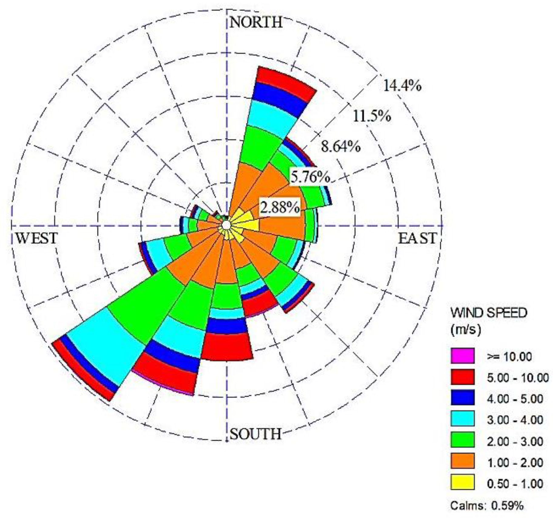
For characterizing the city meteorology, wind data over the year 2019 were collected by the meteorological station located at the Research Centre ENEA of Portici (Figure 1). By analyzing these data, the city results to be characterized by breeze regime as the most coastal areas. Prevailing winds are from S to SW, especially during Spring and Summer and from N to NE, mainly in Autumn–Winter. The most frequent classes of wind velocity are the 1–2 m/s one with an occurrence of 43.3%. It is more frequent than other classes as 0.5–1 m/s and 2–3 m/s with a percentage of 23.8% and 22.3% respectively. The occurrences of wind direction from W to N are rare (Figure 2).

2.2. Building the Urban Geometry and Road Network

For estimating the suitability of urban sites for the deployment of a network of low-cost traffic-orientated stations, the first step was to generate the selected geographical variables as suitability factors.

At this scope, first a 3D model of the city (i.e., buildings and trees) was generated by processing LiDAR data [21], through the Local 3D Government Basemaps tool, an extension of the ESRI-ArcGIS Pro software [22].

To do that, a step-by-step GIS-based procedure was performed. The first step was the point classification of LiDAR point clouds essentially in ground, building and vegetation. Then, Digital Elevation Models (DTM—Digital Terrain Model, DSM—Digital Surface Model and nDSM given from the difference between DSM and DTM) were extracted from classified LiDAR. By processing the DSM, using the Extract Building Footprints tool, a building footprint layer (Figure 3) was generated with associated geometric attributes as buildings perimeter and area.

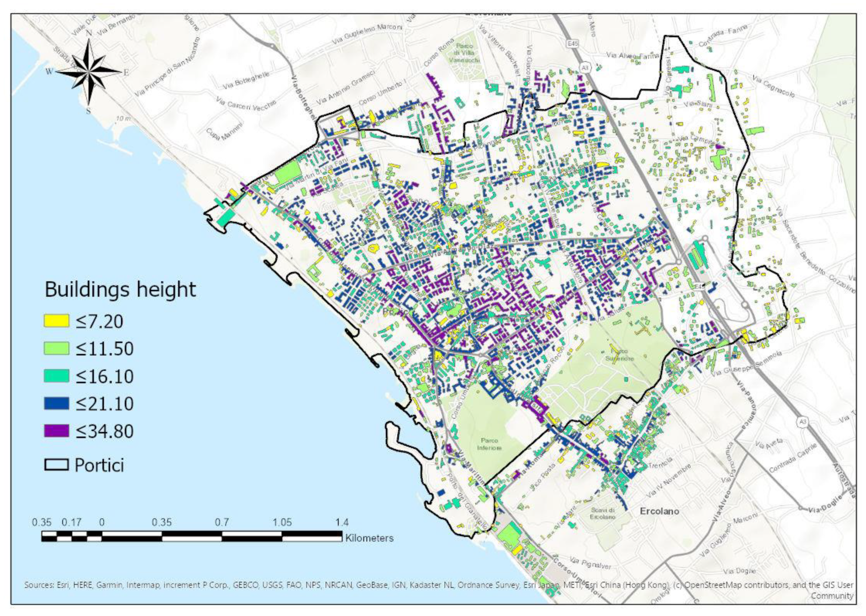
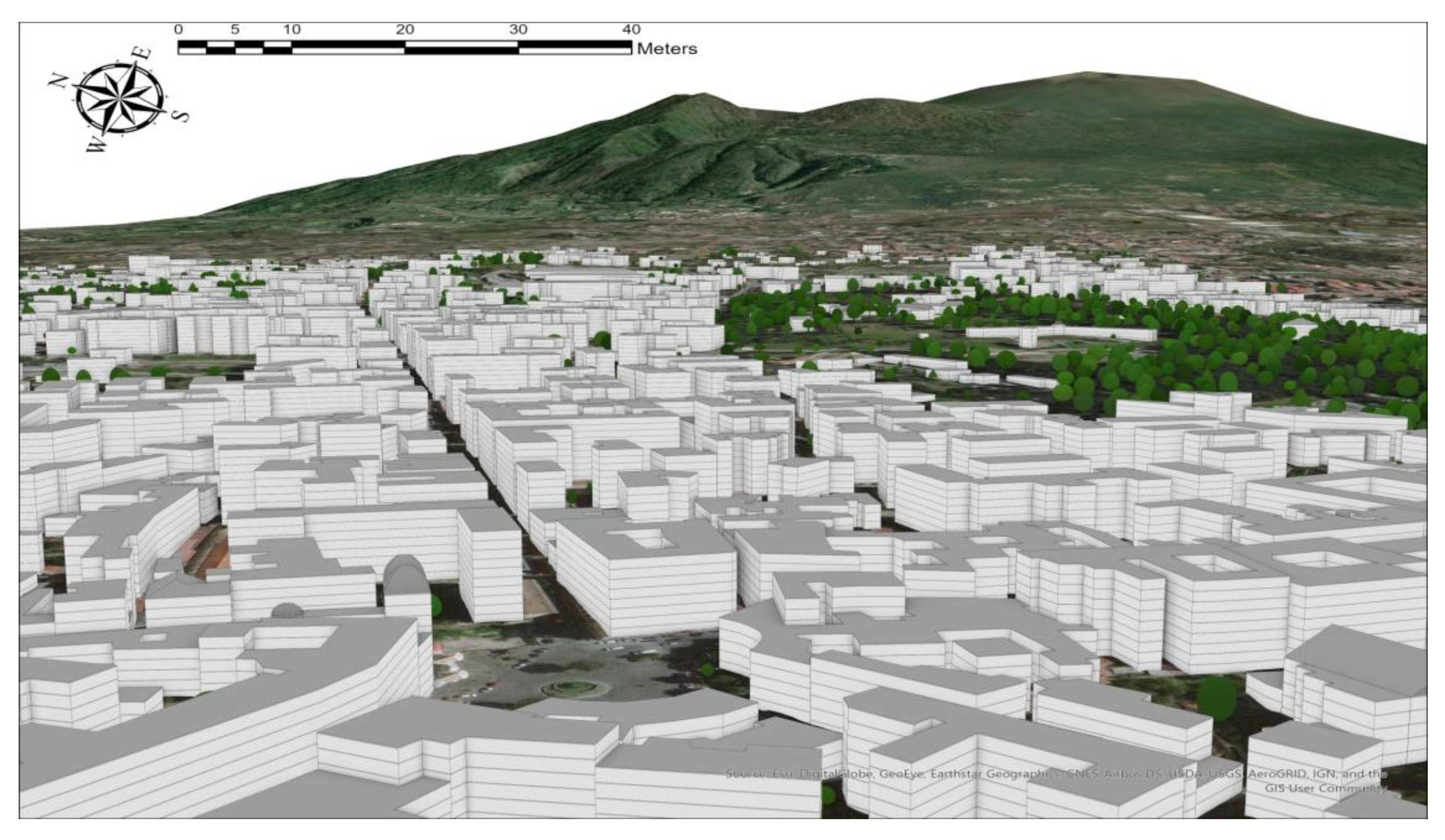
These input raster layers were processed by the Create Buildings and Create Schematic Trees tools of the Local 3D Government Basemaps extension. So, a 3D urban model including buildings and trees was extracted (Figure 4) and the building height attribute was calculated.

The 3D building model was interactively validated by using the images of Google Earth and specific footprint segmentation tools.

The 3D building model obtained counts 2467 buildings with a mean height of 12.97 m and a total surface of 118 km².

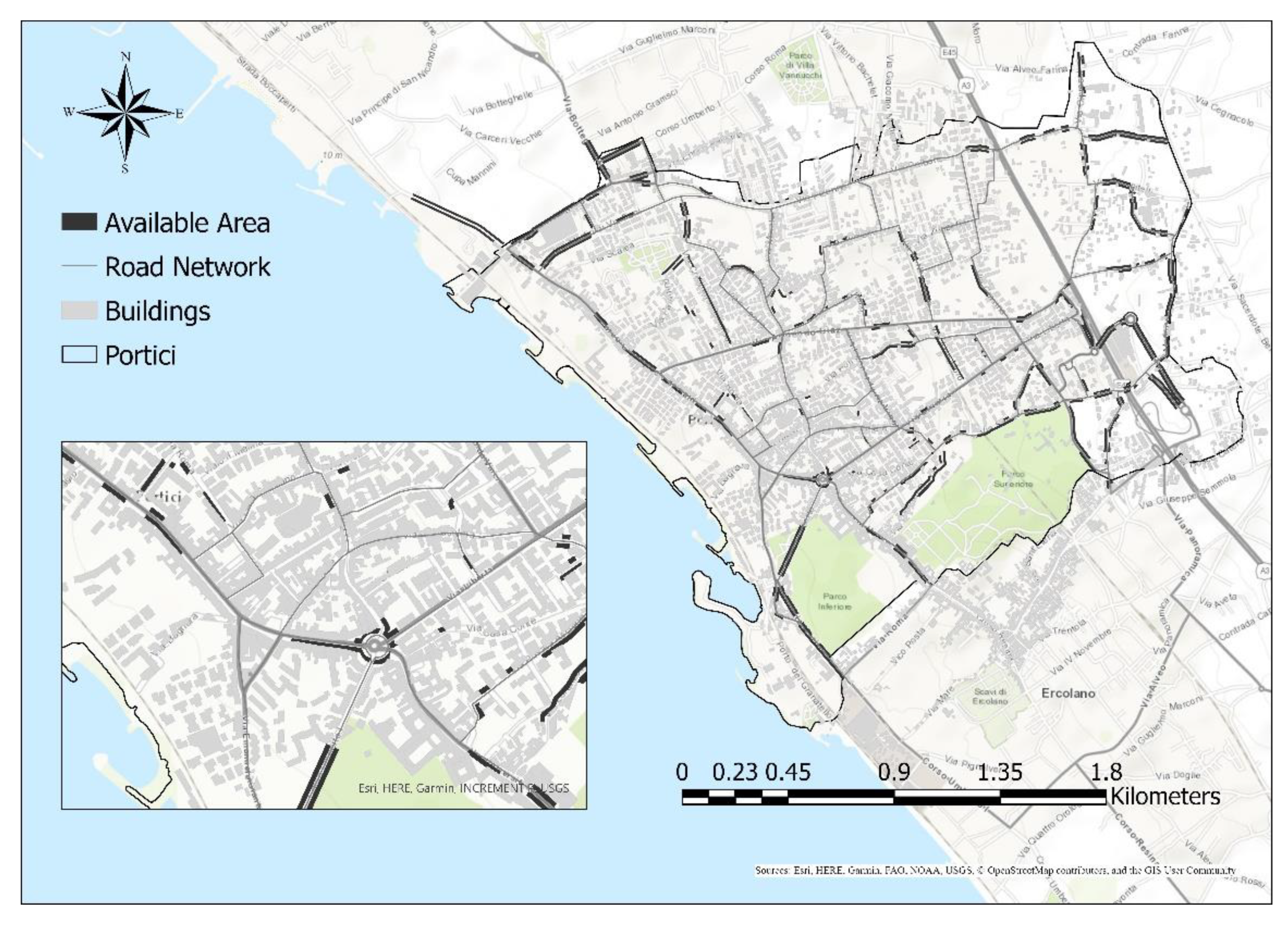
After building the urban geometry, the layer of the urban rood network was collected by the open source geodatabase of the National Geoportal [21] with associated geometric attributes as width and length for each road section. Geometry and topology of this network was interactively validated through the Google Earth images and field surveys.

By combining the layers of urban geometry and the road network, the street canyon layer (Figure 5) was generated by the related building height and road width attributes. This layer classifies the road sections as street canyon or open road.

An urban street affected by street canyon is characterized by a very limited dispersion of pollutants due to the buildings that delimit the road or by an increase in concentrations near the ground due to the phenomena of recirculation that lead to a stagnation of pollutants.

The street canyon effect is generally defined as the aspect ratio W/H, where W is the street width and H is the building height.

It is to be noted that the flow field and the dispersion of the pollutants in a street canyon depend on the geometry of the street canyon but also from meteorological conditions especially wind speed and direction. In this study, we adopted a simplified definition of street canyon geometry based on a threshold value used in the air urban pollutant dispersion model SIRANE [23]. So, the road sections were classified as affected by street canyon if W/H 3 otherwise as open road. In doing so, it was reasonable not considering explicitly the effects of wind speed and wind direction, keeping it for a future more detailed study.

2.3. Modeling Vehicular Flow

The traffic emissions variable was the second criterion selected to identify suitable sites. For generating this variable, the first step was to simulate the vehicular flows along the urban road network and on the basis of these, the related pollutant emissions were calculated.

To do that, the first step was the development of a transportation system model. Identifying a transportation system means to define elements and relationships which let the system to be analyzed [24]. This was realized in three steps: (a) identification of relevant spatial dimensions with the definition of the study area and subdivision of the city into a number of discrete geographic units, commonly called zones; (b) identification and characterization of relevant infrastructural elements, and consequent definition of a network model; and (c) identification of relevant temporal dimensions and definition of relevant characteristics of the travel demand. The link flows can be then computed by assigning the demand flows to the network; by using link cost functions, link mean speeds can be computed from link flows.

Zoning was performed starting from the 119-census geographic units provided by ISTAT (Italian National Institute of Statistics). The use of census units allows each zone to be associated with statistical socio-economic data (e.g., population, employment, daily trips, etc.) that ISTAT makes available for such areas. The aggregation was made considering the physical geographic separators and the homogeneity of zones in terms of use of land and access to transportation services. Nineteen internal zones and twelve external zones were obtained; external zones represent the points where the city is supposed to exchange trips with the external territories.

The defined road network layer was here integrated by characterizing the road sections with performance parameters as free flow speed, capacity of lanes, allowed turns at intersections, among others.

A travel-demand flow is defined as the number of users, with specific characteristics that consume a specific transportation service in a given period of time (typically one hour at this modelling level). Travel demand flows result from the aggregation of individual trips, defined as the act of moving from one site (origin) to another (destination) through the study area during the reference period. The result of this aggregation is the so-called Origin–Destination (OD) Matrix.

Individual trips are generally aggregated on a zone basis, then the OD Matrix resulted as a 31 × 31 matrix composed by a 19 × 19 matrix of internal trips; a 19 × 12 (internal–external) and 12 × 19 (external–internal) trips, commonly called exchange trips; and a 12 × 12 of crossing trips. The estimation of OD Matrix was made starting from data provided by ISTAT for each census unit (the number of employees and the daily trips that people commit internally and externally their residential municipality). For defining an OD-matrix for private transportations (vehicles) in specific hours (morning (07.30–08.30), ante-meridian (12.00–13.00), and evening (17.30–18.30) periods), we calibrated some coefficients useful to extract this information from the ISTAT aggregated data. Specifically, we started from transportation surveys to determine the daily trend of trips, the percentage of trips made with cars, and the percentage between systematic and no systematic trips. Based on the different combination of these values, a 36 OD-Matrix was generated for morning and a 27 OD-Matrix for both, ante-meridian, and evening. Each matrix was assigned, by using an equilibrium assignment methodology, to the basic network and the volumes on each links was calculated.

It is worth noting that also a campaign of traffic survey was conducted for determining the flows circulating in specific sections of the network (on internal and cordon links). Relief measurements was carried out in the months of May and October, counting both during the weekdays (Monday–Friday) and holidays (Saturday–Sunday). Then, results of the simulations were compared with real traffic data in the internal counts section in order to choose the best OD-Matrixes among those generated for each period of time.

By processing this procedure, we calculated the simulated vehicular traffic flows along the urban road network for a typical workday of May and October in the morning, ante-meridian, and evening hours.

Analyzing these layers, we observed that there were minor fluctuations among traffic in the two months considered, and indeed the simulated values were relatively similar. Thus, for our suitability analysis, we considered as representative vehicular traffic flows for a typical workday selecting those related to October.

Moreover, it is to be noted that according to the traffic variation pattern, for a typical workday, the traffic follows a pattern where the peak hour is between 07:30 and 08:30, when most people go to work. Another peak occurs between 12:00 and 13:00, which denotes mobility from people working in the afternoon. A last traffic peak is detected between 17:30 and 18:30, when workers return to their homes. However, the traffic and the associated emissions are higher than the rest of day between the 12:00 and 13:00. So, as representative traffic flows and related pollutant emissions layers, we selected those simulated in the ante-meridian hours.

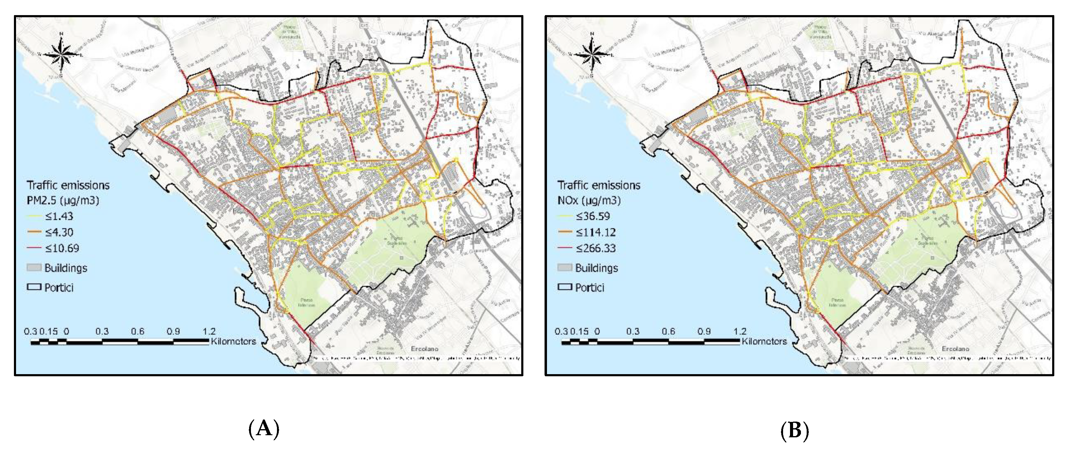
Once defined the traffic volumes and mean speeds on each link, we used these values as input for the calculation of related traffic emissions. The emissions were calculated using the COPERT method [19] where there is a distinction in emissions processes (hot, cold-start, and evaporation). In particular, the emissions were calculated for air pollutants PM2.5 and NOx, according to our case study (Figure 6).

2.4. Clustering the Pollutant Emissions

Traffic-related emissions are the principal source of the local variation in the concentrations of urban air pollutants. In order to capture this variability in our site suitability analysis, local spatial patterns within the simulated traffic pollutant emissions was quantified through a hot-spot analysis based on the Getis-Ord Gi* statistic [25,26].

This spatial analysis works by looking at each feature (e.g., street segment with associated emission values) within the context of neighboring features. A feature with a high value is interesting but may not be a statistically significant hot spot. To be a statistically significant hot spot, a feature has a high value and be surrounded by other features with high values as well. The local sum for a feature and its neighbors is compared proportionally to the sum of all features; when the local sum is very different from the expected local sum, and when that difference is too large to be the result of random chance, a statistically significant z-score results (z standard deviation).

Then, the used Getis-Ord Gi* method works by defining the null hypothesis of complete spatial randomness (CSR) of the emission values associated with the road segment features. Thus, it evaluates the z-score (standard deviation) and p-value (probability that the spatial pattern derives from a random process) values for each spatial feature on the basis of which the null hypothesis is or not rejected. That means to evaluate if rather than a random pattern, the values under examination show a statistically significant clustering. Finally, it aggregates the features in confidence level bins. In particular, features in the +/−3 bins reflect statistical significance with a 99 percent confidence level; features in the +/−2 bins reflect a 95 percent confidence level; features in the +/−1 bins reflect a 90 percent confidence level; and the clustering for features in bin 0 is not statistically significant.

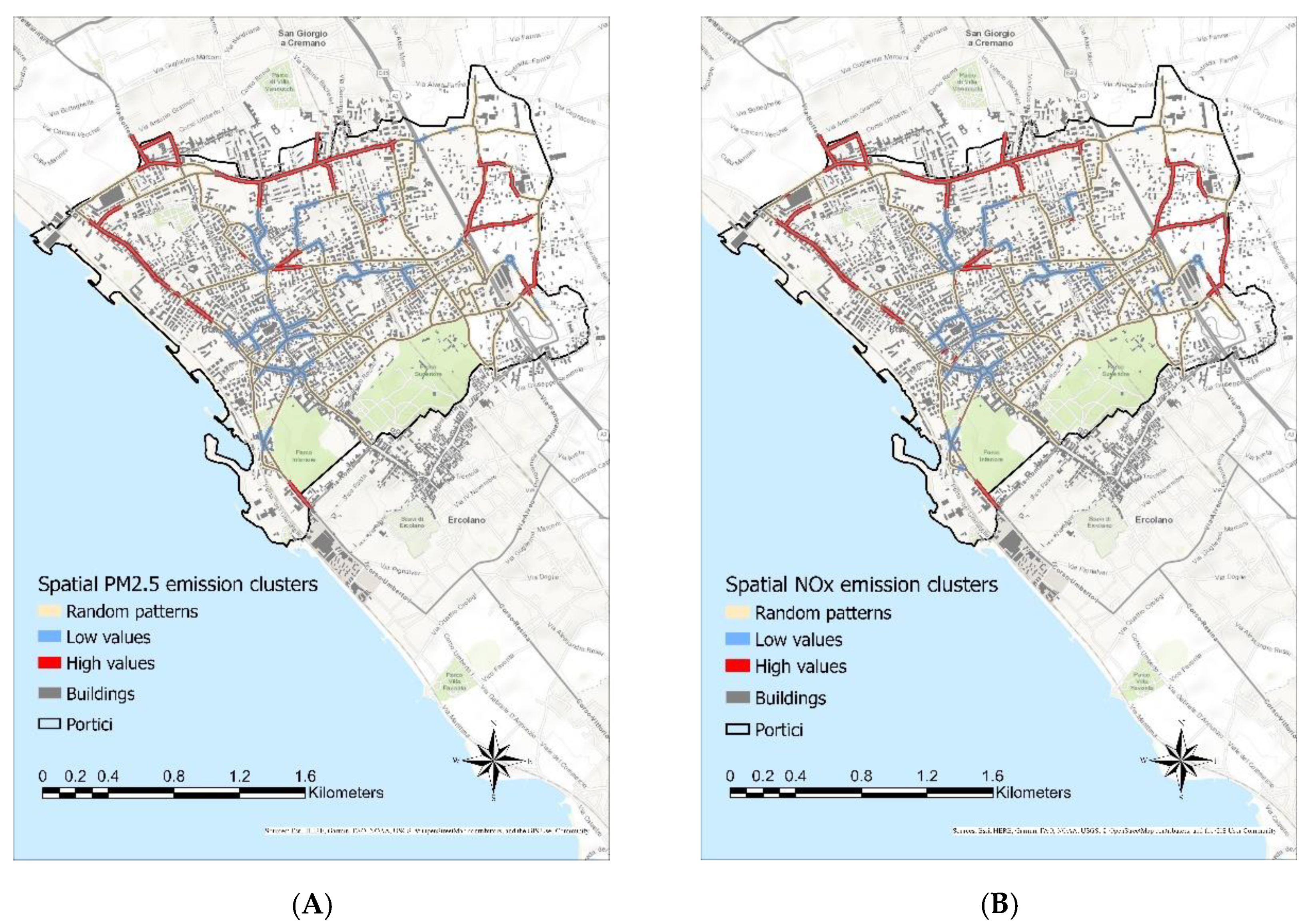
So, through this analysis, statistically significant spatial clusters of high values and low values of the simulated traffic-related emissions as well as random patterns of these ones were identified. From this spatial clustering analysis, a zoning map (Figure 7) of the road network was generated respect to the traffic-related emissions. In particular, the road network was classified in zones at high- and low-emissions and in hybrid zones. The latter do not exhibit spatial pattern of the pollutant emissions. The traffic emission zoning layers, generated for the NOx and PM2.5 emissions and properly combined, represent the other criterion involved in the proposed site suitability analysis.

3. Results

3.1. Site Availability Map

A fundamental step in the proposed procedure is to identify the available sites across the city for deploying a network of low-cost traffic-orientated samplers. The latter are extracted from the urban area according to the location constraints of the air pollutant samplers, established by the regulatory guidelines.

For our scopes, we selected three main location constraints among others. The first of these established that the traffic-orientated samplers were installed at least 25 meters from the edge of major junctions as well as traffic lights, car parks and bus and subway stops. The second one fixed that they were located at least four meters from the center of the nearest traffic lane. According to the third constraint, the samplers had to located no more than 10 meters from the kerbside.

So, for evaluating these constraints, an overlay analysis was performed by overlaying (clipping) the urban area with the building footprints, 4-meter buffer area around the center of the traffic lanes, and a 10-meter buffer area around kerbside, as well as 25-meter buffer area around major junctions, traffic lights, car parks, and bus and subway stops. The final result was a layer of available sites near the roadways (Figure 8). In particular, a number of 274 available sites was identified across the street network of the city on which a network of low cost traffic-orientated samplers can properly be installed for monitoring urban air pollutants.

3.2. Site Suitaility Map

Once identified the available sites, their suitability to allocate a network of stationary low cost traffic-orientated stations, able to capture the local spatial variability of NOx and PM25 concentrations across the city, had to be evaluated with regard to the two defined geographical variables, the street canyon effects and the traffic-related emissions.

In particular, for our scopes, the presence of street canyons and high traffic emissions along the roads meant high suitability. Instead, the presence of street canyons and low emissions meant a moderate suitability. Similarly, we defined the presence of open road and high emissions as moderate suitability while the presence of open road and low emissions as low suitability. Finally, we defined essentially non suitability respect to the emission values which do not exhibit spatial local patterns.

To do that, a GIS-based suitability analysis was performed by combining across all candidate locations the derived layers of traffic emissions of NOx and PM2.5 and the street canyons. For each layer, each class is assigned a score representing the suitability degree to hold a low-cost station. In particular, hybrid-, low-, and high-emission zones are assigned scores ranging from 0 to 2, respectively. Similarity, the road sections affected by street canyon are assigned score 2 while the open roads are assigned score 1. Applying the weighted linear addition (WLA) technique as weighted sum of the ranked (raster) layers, the individual layers were integrated in one layer estimating the overall suitability at each location, ranging from 1 (non- suitable) to 4 (very suitable) All layers were assigned weights equal to 1. Two site suitability maps were generated for low cost NOx and PM2.5 monitors, respectively. Then, they were combined by per-cell statistics raster function (i.e., minimum statistic), deriving the site suitability map (Figure 9) for the deployment of a network of low-cost NOx and PM2.5 multi-sensor stations across the city.

Thus, though this suitability analysis, a number of 169 suitable sites was identified by the available sites, resulting 16 sites highly suitable and 73 sites moderately suitable. Collectively, they represent 53% of the suitable sites. Then, these sites are distributed across the city, more densely around the entry and exit points into the city as shown from the Figure 9.

The statistics about suitable sites are shown in the

Table 1. Statistics of suitable sites for the deployment of a low cost stations network.

Suitability Level	N. Sites	%
Low	80	47
Moderate	73	43
High	16	10

.

From the obtained suitability map, different optimal placement schema can be extracted meeting specific technical and economic requirements for deploying networks of low cost stations able to capture the local spatial variability of pollutants concentration across the city.

4. Discussion and Conclusions

Starting from information about emissions patterns and urban form, by applying a suitability analysis, we were able to identify air quality hotspot areas supposed to show high spatial variability.

In doing so, we are now able to discover the most informative locations in which to deploy the air quality stationary analyzers, maximizing the informative content and power of their measurements.

Thus, optimal deployment algorithms can exploit this outcome, concentrating most of the resources within the hotspot areas. Low cost monitoring stations, there located, will be capable to adequately convey information on areas on which space variability is significant, providing that informative content which is actually lacking for both regulatory monitoring networks and modelling based approaches for air quality mapping. More precisely, this information could be fundamental in data assimilation approaches aimed at including the variability patterns of air pollutant concentrations that conventional chemical transport models or land use regression models fail to adequately represent. This approach could be easily generalized to take into account both spatial and temporal variability pattern of air pollutant concentrations.

It is evident that the high granularity of measurements that results from this approach is made possible by availability of low-cost monitors. Though the collected data quality has still to be investigated, networks of these monitors, properly located according the defined suitable sites, allow to address a spatially dense air quality monitoring across a city, ensuring a more reliable urban air quality management with lighter installation and maintained costs.

It is to be noted that the proposed methodology may result in too few high suitability sites. In this case, the inherent flexibility of the method may allow to enlarge the selected sites set by taking into account moderate suitability sites until the desired density will be reached.

Moreover, the generality of the proposed methodology may also allow its adoption for the selection of suitable sites for reference instruments of the current regulatory air quality monitoring networks which is also a topic on which there is no agreement at the moment.

One of the possible limitations to the use of the proposed methodology is its reliance on data could be difficult to obtain such as vehicular flow (simulated or measured) as well as the street canyon effects. In this cases, the use of proxy data could partially solve the issue.

5. Future Work

During this study, some future developments have been identified which could result in more accurate site suitability calculation. First of all, the calculation of the available sites for deploying low cost monitors that includes the shadow effect of buildings and trees as well as the evaluation of minimum winter solar radiation value to be ensured, as further location constraints. In fact, low cost monitors are generally equipped with a photovoltaic panel and a battery storage and installed on existing street lighting poles. Including these constraints should allow to select sites with a better sun exposure over the year.

The focus of this study was on the traffic-orientated stations. As further development, the site suitability analysis could be extended to combined networks of low-cost traffic and background stations. To do that, appropriate location constraints (e.g., far away from roads) and geographic variables have to be defined for quantifying the integrated contribution of several pollution sources located in downwind areas respect to the site and respect to predominant wind direction in the site.

Finally, the meteorology could be explicitly considered as within air pollutant dispersion model.