Abstract
As one of the most polluted U.S. cities, Fairbanks was reclassified as a “serious” nonattainment area by the Environmental Protection Agency (EPA) in 2017 for its fine particulate matter (PM2.5) pollution. In this study, November 2013–May 2019 observations of criteria air pollutants (NO2, SO2, CO, O3, PM2.5, and inhalable particulate matter (PM10)) and meteorological parameters (temperature, wind speed, and relative humidity) in Fairbanks were used for temporal variation and correlation analysis, with positive matrix factorization (EPA PMF 5.0) adopted for further PM2.5 source identification. All pollutants exhibited obvious seasonal trends under the influence of climatology, topography, and human activity, while abnormal patterns likely resulted from occasional emission events such as wildfires. Primary and secondary pollutants performed distinctively under similar meteorological conditions due to different decisive factors. Identified PM2.5 sources included sulfate (32.7%), wood smoke (19.3%), gasoline (18.3%), nitrate (15.7%), diesel (9.2%), soil (3.8%), and road salt (1.0%). Compared with the 2005–2012 result, sulfate and nitrate contributions had increased, while wood smoke and diesel contributions had decreased, in which emission control measures as well as a change of sampling sites could play an important role. This systematic analysis offers reference for mitigation measures and pollution prediction. Meanwhile, further field investigation is required for conclusion validation and model improvement.
1. Introduction
Fairbanks, Alaska has been suffering severe air pollution, especially PM2.5 pollution in the past few years. In October 2009, part of the Fairbanks North Star Borough was designated as nonattainment according to the 2006 24-h PM2.5 National Ambient Air Quality Standard (NAAQS), and the area was reclassified from “moderate” to “serious” nonattainment in May 2017. Meanwhile, such pollution can induce numerous respiratory and cardiovascular diseases [1], which threatens the health of local residents.
Previous air quality studies in Fairbanks mainly focused on the dominant pollutant of PM2.5, including source apportionment and pollution-forming conditions. For source apportionment, Ward et al. [2] identified five factors including wood smoke, sulfate, automobiles, ammonium nitrate, and diesel exhaust with the Chemical Mass Balance (CMB) model, based on winter observations (2008–2009, 2009–2010, 2010–2011) at four sites in Fairbanks. Using the Positive Matrix Factorization (PMF) model, Wang and Hopke [3] identified wood smoke, sulfate, gasoline, diesel, nitrate, soil, and road salt as possible sources through the analysis of 2005–2012 data. Both researches reported wood smoke and sulfate as the first and second largest PM2.5 contributor in winter, while differences existed in the types, number, and proportions of other sources. Such disparity probably resulted from the exclusion of November data for winter in the latter study [3]. Apart from the common sources mentioned above, hydrogen sulfide (H2S) and ammonia (NH3) emitted by hot springs around Fairbanks can also serve as precursors of ammonium and sulfate aerosols [4], which are important components of secondary PM2.5. For pollution-forming condition, according to Tran and Mölders [5], a combination of surface inversion, calm wind, low temperature, and low humidity traps PM2.5 in the breathing level and inhibits the transportation of polluted air out of Fairbanks in winter, stressing the importance of topographical and meteorological factors in modulating air pollution. When it comes to anthropogenic influence, the impacts of emission control measures (e.g., wood-burning device changeout, introduction of gas, and low-sulfur fuel) on near-surface PM2.5 concentrations for a cold season in Fairbanks was analyzed using WRF/Chem simulations and 2008/2009 hourly observations by Mölders [6]. Replacing wood-burning by gas would reduce PM2.5 emission by ≈11%, while the changeout of uncertified wood-burning devices would bring about a ≈4% decrease. The indirect measure of introducing low-sulfur fuel would reduce SO2 and PM2.5 by ≈23% and 15%, respectively [6].
Nevertheless, interactions of other criteria air pollutants (NO2, SO2, CO, O3, and PM10) with PM2.5 under specific meteorological conditions are also crucial and need further exploration, for they involve PM2.5 formation as precursors or co-products. In this study, we investigated temporal variations of six criteria air pollutants (NO2, SO2, CO, O3, PM2.5, and PM10) and meteorological parameters (wind speed, temperature, and relative humidity) as well as their mutual correlations in Fairbanks, based on daily observations from November 2013 to May 2019. Meanwhile, PM2.5 was ulteriorly analyzed through source apportionment, and results were compared with previous research using 2005–2012 observations [3]. This systematic long-term analysis raised possible interpretations of pollutant forming mechanisms in Fairbanks from different aspects, offering reference for mitigation measures as well as pollution prediction.
2. Experiments
2.1. Study Area
As the largest city in interior Alaska, Fairbanks possesses a total area of 85 km2 and a population of 31,516 (2018 estimates). Lying just 196 driving miles south of the Arctic Circle (Figure 1), its climate is classified as subarctic with long cold winters and short warm summers. Winter usually lasts from late September/early October to late April/early May. Normal monthly mean temperatures range from −22.2 °C in January to 16.9 °C in July. Due to Fairbanks’ location at the bottom of the Tanana Valley, in winter, cold air accumulates in and around the city, while warmer air rises to tops of the hills in the north [7], causing surface inversion for more than 95% of the time. In summer, inversions occur relatively seldom [8].
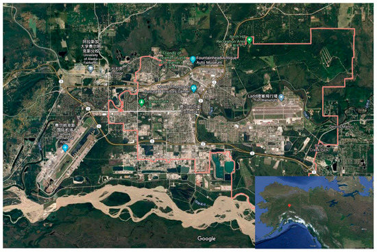
Figure 1.
Study region. Map in the bottom right corner shows the NW North American outline, with Fairbanks marked by the red teardrop. (Maps from https://www.google.com/maps).
2.2. Data Acquisition and Pretreatment
Concentrations of six criteria air pollutants (NO2, SO2, CO, O3, PM2.5, and PM10) as well as 21 PM2.5 species (Al, NH4+, Br, Ca, Cl, Cr, Cu, EC1, EC2, Fe, Mg, OC1, OC2, OC3, OC4, K, Si, Na, S, NO3−, and Zn) were provided by the National Core Network (NCore) site (809 Pioneer Rd.) in Fairbanks. Criteria air pollutants were measured daily according to designated federal reference method (FRM) and federal equivalent method (FEM) [9]. For PM2.5 speciation, organic carbon/elemental carbon (OC/EC), major ions, and trace metals were collected with quartz, nylon, and teflon filters on the spiral ambient speciation sampler (SASS, Met One Inc., Grants Pass, OR, USA), and measured using thermal optical reflectance (TOR), ion chromatography (IC), and energy-dispersive X-ray fluorescence (EDXRF), respectively [10]. Data of PM2.5 species were provided every three days. Daily meteorology data (temperature, relative humidity, and wind speed) were provided by the Fairbanks International Airport Station. Negative and zero concentrations of criteria air pollutants were excluded, while those in PM2.5 speciation were retained and treated as below detection limit (BDL) values. Detailed information of sample sites, sample period, and data sources is shown in Table A1.
2.3. PM2.5 Source Apportionment
Positive matrix factorization (PMF) [11] was adopted for source apportionment, and EPA PMF 5.0 was used in this study. Concentrations and uncertainties of below detection limit (BDL) and missing data were calculated according to Polissar et al. [12]. Species with a signal to noise ratio (S/N) larger than 1.0 included NH4+, Ca, Cl, Cu, EC1, EC2, Fe, OC1, OC2, OC3, OC4, K, Si, S, NO3− and Zn, and they were classified as “strong”. Species whose S/N were larger than 0.5 and less than or equal to 1.0, including Br, Na, Mg, Cr, and Al, were classified as “weak” and down-weighted by a factor of 3. Given the higher missing rate of EC1, EC2, OC1, OC2, OC3, and OC4 measurements (Table A1), their uncertainty parameters were set to 15, while those of other species were set to 10. No extra modeling uncertainty is used. Trials with six to nine factors were conducted. Displacement analysis (DISP) was conducted for exploring rotation ambiguity [13], and rotations using Fpeak values of −1, −0.5, 0.5, 1, and 1.5 were introduced [14]. More details of PMF input and output are provided in Appendix B.
2.4. Statistical Methods
Normality of data distribution was examined using the Anderson–Darling test (Table S1). Since the climatological parameters, criteria air pollutants, and PM2.5 speciation do not follow the normal distribution, we used Spearman’s correlation coefficient for analysis. Correlation significance results are shown in Tables S2–S4 and S8.
3. Results and Discussion
3.1. Data Overview
Table 1 and Table 2 provide arithmetic mean, maximum, median, minimum, standard error (SE), and count of criteria air pollutant and meteorological variable observations in Fairbanks within the study period. The maximal concentration of PM2.5 is higher than that of PM10, due to the missing of PM10 observation on the day when PM2.5 reached maximum. Table 3 provides arithmetic mean, SE, geometric mean, method detection limit (MDL), BDL data percentage, and missing data percentage of PM2.5 and PM2.5 speciation.

Table 1.
Statistical summary of daily average concentrations of six criteria air pollutants (μg/m3 for PM2.5 and PM10, ppb for SO2, NO2, O3, and CO) in Fairbanks from November 2013 to May 2019. (SE: standard error) Measurements with negative observations are excluded. Maximums of PM2.5 and PM10 did not appear on the same day.
Table 2.
Statistical summary of daily average measurements of wind speed (WS, m/s), temperature (T, °C) and relative humidity (RH, %) in Fairbanks from 3 November 2013 to 30 May 2019. (SE: standard error).
Table 3.
Statistical summary of PM2.5 species concentration (μg/m3) in Fairbanks from November 2013 to May 2019 (BDL: below detection limit; MDL: method detection limit). Samples were collected every three days. The August–December 2014 period with no species measurements has been excluded. The geometric mean was calculated using data above the MDL.
3.2. Temporal Variations of Air Pollutants and Meteorological Parameters
Figure 2 and Figure 3 show seasonal variations of meteorological parameters and air pollutants. For meteorology, wind speed was higher in spring and summer and reached a minimum in winter. Average daily temperature in summer and winter were the highest and the lowest, respectively, while spring and fall had similar values. Relative humidity showed an increasing trend from spring to winter. Clear annual variations were also observed for all pollutants. Concentrations of SO2, NO2, CO, PM2.5, and PM10 peaked in winter, when strong and semi-permanent inversion separates the boundary layer from the air aloft [15], which together with increased emission leads to the accumulation of combustion-originated pollutants. Values in spring and fall were close with only a slight difference in data distribution, and minimum concentrations appeared in summer. Meanwhile, O3 peaked in spring and reached a minimum in winter, showing a decreasing trend similar to that of relative humidity. This prompts that apart from topography and human activities, meteorological factors may also play an important role in influencing pollutant concentrations, which needs further exploration. Distinctions between variation trends of the primary pollutants (SO2, NO2, and CO) and secondary pollutant (O3) indicate different decisive factors in modulating their concentrations. Pollutant distributions in different wind directions are not included in this study due to the low explanatory power of wind direction in pollutant variations.
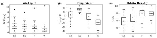
Figure 2.
Seasonal variations of (a) wind speed (b) temperature (c) relative humidity (Sp—spring; Su—summer; F—fall; W—winter). The central box represents values from lower to upper quartile (25th to 75th percentile). The vertical line extends from the 10th percentile to the 90th percentile. The middle solid line represents the median. The gray diamond represents the arithmetic average. Maximal and minimal outliers are plotted as black dots.
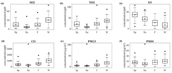
Figure 3.
Seasonal variations of (a) SO2 (b) NO2 (c) O3 (d) CO (e) PM2.5 (f) PM10 (Sp—spring; Su—summer; F—fall; W—winter). The central box represents values from the lower to upper quartile (25th to 75th percentile). The vertical line extends from the 10th percentile to the 90th percentile. The middle solid line represents the median. The gray diamond represents the arithmetic average. Maximal and minimal outliers are plotted as black dots.
Figure 4 and Figure 5 show monthly average variations of meteorological variables and pollutants within the study period, respectively. Apart from aforementioned seasonal trends, abnormal patterns also appeared in specific years. In summer 2015, there were peaks of CO, PM2.5, and PM10, which are dominant pollutants emitted by forest fires in quantity [16], as shown in Table S5. The period with extreme CO and particulate matter concentrations matched the Aggie Creek Fire (Figure 6), which was located 30 miles northwest of Fairbanks and consumed an estimated 31,705 acres within about a month [17]. This suggests that in Fairbanks, the co-occurrence of excessive CO and particulate matter in summer can be a strong indicator of wildfires as a result of incomplete vegetation combustion.
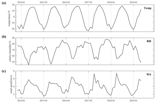
Figure 4.
Monthly average variations of (a) temperature (b) relative humidity (c) wind speed from November 2013 to May 2019 (Temp—temperature; RH—relative humidity; WS—wind speed). Gray dashed lines represent January of each year.
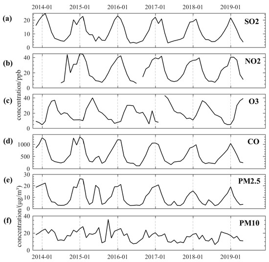
Figure 5.
Monthly average concentration variations of (a) SO2 (b) NO2 (c) O3 (d) CO (e) PM2.5 (f) PM10 from November 2013 to May 2019. Gray dashed lines represent January of each year.
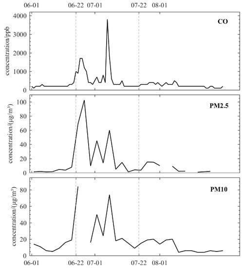
Figure 6.
Variations of CO, PM2.5, and PM10 concentrations in Fairbanks during summer 2015. The first gray dashed line marks the start date of the Aggie Creek Fire. The region between the two gray dashed lines is the approximate lasting period of the fire. CO was sampled daily within the period. PM2.5 and PM10 were sampled every three days within the period.
3.3. Correlation Analysis
3.3.1. Correlations between Air Pollutants
Table 4 shows the overall and seasonal relationships of six criteria air pollutants quantified with Spearman’s correlation coefficient (ρ). Daily concentrations were used for calculation. Correlations with coefficients less than 0.3 were regarded as weak and ignored. For yearly results, all correlations are statistically significant. NO2, SO2, CO, PM2.5, and PM10 were highly positively correlated (ρ > 0.5) with each other, which is consistent with their similar seasonal variation patterns and may suggest a common source [18]. Noteworthily, correlation coefficients between PM2.5 and the combustion-originated pollutants were all greater than 0.70, indicating the considerable contribution of fuel burning to PM2.5 formation in Fairbanks. Among all, correlation between PM2.5 and CO was the strongest (ρ = 0.82). Given the high proportion of carbonaceous matter (e.g., OC/EC) in PM2.5 [10], such strong correlation probably resulted from the co-production of CO and OC/EC through incomplete biomass or fossil fuel combustion. Meanwhile, O3 was strongly anti-correlated with PM2.5 and CO, while it was moderately (0.3 ≤ ρ < 0.5) anti-correlated with SO2 and NO2. For negative correlation between O3 and PM2.5, low PM2.5 concentration can lead to stronger solar radiation, which promotes O3 formation [19,20]. Plus, explanation for negative correlation between O3 and NO2 can be mutual transformation through photochemical reaction.
Table 4.
Annual and seasonal correlations of six criteria air pollutants in Spearman correlation coefficient. Daily measurements were used for calculation. Strong correlation: |ρ| > 0.5; moderate correlation, 0.3 < |ρ| < 0.5; weak correlation, |ρ| ≤ 0.3. Number of stars represent significant levels. (*** p-value < 0.001; ** p-value < 0.05; * p-value < 0.1).
Correlation patterns in spring, fall, and winter were alike despite slight changes in correlation significance, suggesting the plausibility of dividing a year into warm and cold seasons [4] rather than the usual four seasons according to the characteristic climatology in Fairbanks. In summer, strong positive correlations of SO2, NO2, and CO with PM2.5 had weakened to varying degrees, while the correlation was still significant. Additionally, a weak but significant positive correlation was observed between O3 and PM10, while a strong and significant one existed between O3 and NO2. Positive correlation between particulate matter and O3 in summer may indicate the strengthened formation of secondary particulate matter [18], which is supported by weakened positive correlations between PM2.5 and primary pollutants of SO2, NO2, and CO. Under favorable conditions, NO2 and SO2 can become precursors of nitrate and sulfate, which are major components of secondary PM2.5. This also helps explain the decrease of correlation coefficients in the summer.
3.3.2. Correlations between Air Pollutants and Meteorological Parameters
Relationships between pollutants and meteorological variables were also investigated and are shown in Table 5, and all correlations are statistically significant. Daily measurements were used for calculation. NO2, SO2 CO, PM2.5, and PM10 were moderately to strongly anti-correlated with wind speed and temperature. In addition, CO showed a moderate positive correlation with relative humidity. Negative correlations of NO2, SO2, CO, PM2.5, and PM10 with wind speed indicate the importance of horizontal dispersion in reducing their concentration [21], and according to Tran and Mölders [5], calm wind (average speed < 0.5 m/s) is necessary for the forming of high PM2.5 concentration in winter. Their negative correlations with temperature largely arose from increased heating and electrical powering emissions as well as strengthened inversion in cold weather. Inversely, O3 had positive dependencies on wind speed and temperature while a strong negative one on relative humidity. It is probably because high-speed wind helps remove particulate matter, thereby enhancing O3 formation through photochemical reaction. Meanwhile, high relative humidity promotes O3 absorption by atmospheric moisture, while low temperature slows down its formation rate.
Table 5.
Correlations between six criteria air pollutants and meteorological parameters (T—temperature; WS—wind speed; RH—relative humidity) in Spearman’s correlation coefficient. Daily measurements were used for calculation. Strong correlation: |ρ| > 0.5; Moderate correlation, 0.3 < |ρ| < 0.5; Weak correlation, |ρ| ≤ 0.3. Number of stars represent significant levels. (*** p-value < 0.001; ** p-value < 0.05; * p-value < 0.1).
Since different meteorological features distinguish different seasons, opposite correlations of primary and secondary pollutants with the meteorological variables account for their distinct seasonal variation patterns to a large extent. In winter, growing fuel combustion brings about increased emission of primary pollutants, while inversion and low wind speed inhibit their transportation and lead to their accumulation. For the secondary pollutant of O3, high wind speed and relative humidity contributes to its high concentration in spring.
3.4. PM2.5 Source Identification
As the dominant air pollutant in Fairbanks, possible sources of PM2.5 were explored using receptor modeling. A seven-factor solution was picked based on relative values of Qrobust and Qtheoretical, scaled residual distribution, and profile interpretability, and the base run result (Fpeak = 0) turned out to be the most reasonable. Identified factors include diesel, nitrate, sulfate, wood smoke, soil, gasoline, and road salt (Table 6), whose profiles and temporal variations are shown in Figure 7 and Figure 8. After excluding data points with missing PM2.5 observations and those sampled on violation days (daily average PM2.5 concentration > 35 μg/m³) during the Aggie Creek Fire, PM2.5 predictions and observations were compared in Figure S2, while comparison with the complete data is shown in Figure S3. The regression (R² = 0.998, slope = 0.94) shows that the predictions reproduced the observations effectively when there were no sporadic emission events. Comparison with source apportionment results using 2005–2012 observations [3] was made to figure out possible changes in proportions and compositions of sources.
Table 6.
Annual and seasonal average source contributions. (SE—standard error).
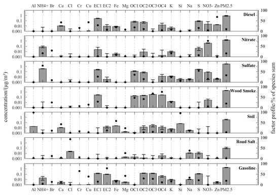
Figure 7.
Source profiles. Bars represent species concentrations in each factor, y-axis on the left. Error bars represent displacement analysis (DISP) intervals, y-axis on the left. Dots represent species contributions, y-axis on the right.
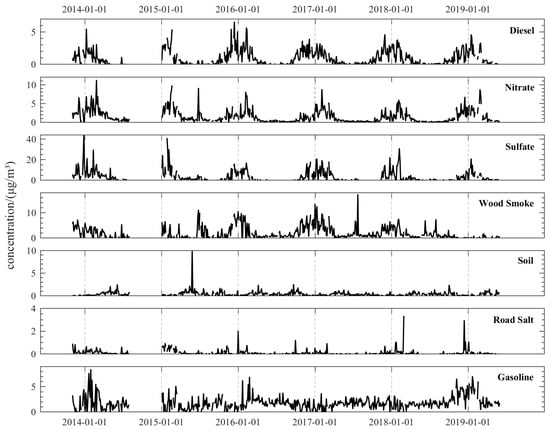
Figure 8.
Temporal variations of PM2.5 source concentrations. Dashed lines represent 1 January of each year.
3.4.1. Sulfate
Sulfate was the major source during the study period, comprising primary and secondary compositions mainly from S-containing fuel combustion. Apart from the representative species of S, NH4+, NO3−, EC, and OC in its profile, DISP analysis also showed tight bounds for K, Na, Zn, and Si. Considering that K and Na are emblematic in biomass burning, residential or industrial co-combustion of S-containing fuel (e.g., coal/diesel/gasoline) and biomass may contribute to K/Na in the sulfate factor, through which sulfur is captured by alkali in plant ash and removed as fly ash [22]. The presence of Zn suggests possible intermixing between diesel and sulfate factors, since Zn is a typical additive of the diesel. Coal consumed in Fairbanks mostly comes from the Usibelli coal mine, and SiO2 is the major component of Usibelli coal ash [23], which could be reason for Si in the profile. The results above illuminate that apart from reducing emissions, proper burning remains disposal is also important for PM2.5 pollution control. Both the concentration and proportion of sulfate reached their maximum in winter, when demand for heating and electrical powering also peaked.
The contribution of sulfate showed a significant increase compared with the 2005–2012 results. Notably, the Aurora Energy Power Plant, which is capable of electricity and heat supply [24], is only 524 m from the monitor station. Such a close distance can explain the increase to some extent, since the previous research used observations from the State Office Building (675 7th Ave) Speciation Trend Network (STN) site, which is about 1 km from the closest coal plant. Contribution in winter had risen, while that in summer had dropped. This reveals possible changes of the sulfate source between the two studies. In this study, coal combustion of the power plant accounted for a large proportion of the sulfate factor, which is strongly influenced by the temperature. The strong and significant negative correlation (ρ = −0.88) between sulfate and temperature (Table S6) can also support this. Meanwhile, the downtown location of the STN site indicates that a considerable amount of sulfate measured here came from traffic emissions and subsequent secondary reactions, which varies less with season.
3.4.2. Wood Smoke
Wood smoke was the second biggest source identified. This factor mainly consisted of EC, OC, K, and NO3−; nevertheless, the DISP interval of NO3− extended to less than 10−3 μg/m3, indicating that NO3− was not the essential component of this factor. The peak value of wood smoke appeared in winter. However, its maximal proportion appeared in summer, as a result of frequently striking festival wildfires around Fairbanks. The obvious peak of wood smoke in summer 2015 confirms our hypothesis that the excessive CO and particulate matter observed within that period came from wildfires. On violation days during the Aggie Creek Fire, wood smoke accounted for 47.15% of reconstructed PM2.5 in average (Figure 9), suggesting that wildfire is the main contributor to PM2.5 exceedance days in summer. In cold weather, wood-fired heating replaced wildfires as the main producer of wood smoke. Considering that relative humidity influences the wood drying rate and thereby smoke produced during combustion, we investigated the relationship between relative humidity and wood smoke factor concentration. A strong and significant positive correlation (ρ = 0.80) indicates that high relative humidity promotes wood smoke production through incomplete combustion (Table S6). This also helps explain the negative correlation between CO and relative humidity, since CO is also typical of biomass incomplete combustion.
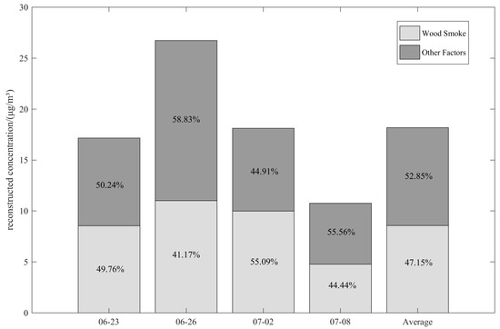
Figure 9.
Percentage of wood smoke factor accounted for reconstructed PM2.5 on violation days during the Aggie Creek Fire.
Contributions of wood smoke in all four seasons had decreased compared with previous research, in which a series of measures to reduce wood smoke production may have played an important role. For the wood stove change-out project, according to the Fairbanks 2013–2015 Home Heating Surveys [25], a fraction of woodstove/insert energy use from uncertified devices had decreased from 23.6% in 2011 to 16.3% over the 2013–2015 period. It was also required that all uncertified wood-fired heating devices in a property should be replaced when the property was sold since 9 June 2017 [26]. This can bring about significant improvement, for certified devices tend to produce half of the PM emissions of their counterparts. Furthermore, the mandatory Wood Seller Registration requirement effective from 15 August 2017 promoted cleaner burning by asking wood sellers to measure moisture before selling wood [27]. The introduction of control measures in 2017 might have conduced to the significant decrease of wood smoke contribution in 2018 (Figure 10).
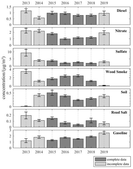
Figure 10.
Annual concentration variations of PM2.5 sources. Dark gray bars represent years with data of every month. Light gray bars represent years with at least one month of missing data. Error bars represent one standard error.
Noteworthily, according to the Fairbanks official report in 2019 [28], wood smoke rather than power plants was the main PM2.5 source in Fairbanks. Such divergence between observations and reconstruction results could arise from the location of the sampling site. Therefore, a further on-site survey is required to investigate wood stove distribution in Fairbanks as well as its possible impact on source apportionment results.
3.4.3. Nitrate
The major components of this factor included NO3−, NH4+, and S, while EC, whose DISP interval extended below 10−3 μg/m3, could be ignored. Noticing the highly overlapping species in nitrate and sulfate profiles, we observed the G-space plot of the two factors (Figure S4). Data points filling the whole scatter plot space indicate there was no significant correlation between nitrate and sulfate. Considering that plantation was limited around Fairbanks, nitrate less likely came from fertilizers, and the major source of nitrate was probably fossil fuel or biomass combustion. In winter, the increased consumption of N-containing fuel from traffic, heating, and powering produces more precursors such as NOx and NH3 [29]. Meanwhile, strong inversion and low wind speed provide stable conditions for gas-phase homogeneous reactions, and low temperature also promotes the combination of NH4+ and NO3−. These together lead to a nitrate peak in winter.
Similar to that of sulfate, the contribution of nitrate had also increased compared with previous results. Apart from the possible influence of changing sampling sites, this could also suggest strengthened secondary PM2.5 formation in Fairbanks, which needs further validation.
3.4.4. Diesel and Gasoline
Diesel and gasoline are typical fuel oil whose primary uses include home heating and vehicle powering. The diesel factor mainly comprised OC, EC, S, NO3−, Ca, Fe, and Zn, while the gasoline factor contained OC, EC, S, and NH4+ chiefly. Although concentrations of both factors peaked in winter, the seasonal variation of gasoline was not as obvious as that of diesel. Such phenomenon suggests that diesel, with a relatively higher caloricity and lower price, took a bigger share in home heating fuel and was consumed more in cold seasons. This is supported by a strong and significant negative correlation (ρ = −0.99) between temperature and diesel concentration (Table S6). Meanwhile, gasoline was used more for powering engines all year round, which resulted in its relatively weaker correlation (ρ = −0.69) with temperature.
The contribution of diesel had decreased compared with the 2005–2012 result, while that of gasoline had changed little. Nevertheless, the reconstructed summer average concentration of diesel turned out to be slightly negative (−0.018 ± 0.015 μg/m3), indicating the possible unfitting part of this factor. In Fairbanks, heating oil is the principal fuel for home heating [25]. Notably, chemical compositions of most home heating oil (HHO) products are very similar to those of diesel, except for the difference in sulfur content [30]. This suggests that part of the diesel factor contribution may actually come from HHO burning exhaust.
3.4.5. Soil and Road Salt
The factor whose profile included Al, Ca, Si, Fe, OC, and EC was classified as soil. Components of OC/EC indicate that apart from crust elements, the soil factor also contained organic particles from incomplete combustion remains, such as coal ash. A large proportion of coal ash in Fairbanks is stockpiled in landfills, and dust can be blown from the disposal sites. According to Petras [31], coal ash sampled in Fairbanks is rich in As, V, and Hg. Despite the unavailability of their concentration data in this study, these elements can serve as marker species to identify the existence of coal ash in the soil factor for future studies.
Concentration of the soil factor peaked in spring, whose climate is characterized by low relative humidity (RH) and high wind speed (WS). Such meteorological conditions promote the desiccation and atmospheric dispersion of soil. This is also confirmed by a strong and significant negative correlation (ρ = −0.80) between the soil factor and RH as well as a strong and significant positive correlation (ρ = 0.84) between the soil factor and WS (Table S6).
The last factor that was enriched in Cl, Na, and S was classified as road salt, and its peak concentration appeared in winter. Contributions of soil and road salt remained relatively stable compared with previous research results.
3.5. Analysis Based on Two-Season Criterion
As mentioned in Section 3.3.1, similar correlation patterns in spring, fall, and winter suggest that it may be more suitable to divide a year into two instead of four seasons. Therefore, we have conducted further analysis based on a two-season division. The cold season, which approximately overlaps with the time range of winter in Section 2.1, lasts from October to April of the next year. Meanwhile, the warm season extends from May to September. The two seasons are most obviously distinguished by a temperature difference of 24.28 °C (Figure S5). The warm season also has higher wind speed and lower relative humidity than the cold season (Figure S5), but the difference is not as significant as that of temperature.
For criteria air pollutant performance, SO2, NO2, CO, and PM2.5 exhibited a significant inter-season difference (Figure S6), while those of O3 and PM2.5 are also obvious but not as significant. Seasonal variation patterns correspond with the conclusions in Section 3.3.2, although the inter-season difference of O3 is actually weaker under the new criterion. This indicates that it may be better to stick to four-season division for O3 analysis, for its concentration peaked in spring, which is split into two parts under the two-season criterion. The correlation patterns of six air pollutants criteria in the cold season is similar to those in fall and winter, while patterns in the warm season are similar to those in summer (Table S7), suggesting that such division did capture the distinction between seasons.
Source apportionment results based on the two-season criterion are illustrated in Table S9. All factors except for gasoline and soil exhibited a clear difference between the warm and cold seasons. For gasoline, this can be related with its usage, as mentioned in Section 3.4.4. For soil whose contribution peaked in spring, it is most probably because of omitting the May and April data as well as introducing data from June to September. This is also reflected by the increased relative humidity in the warm season (Figure S5), considering its influence on the airborne transmission of soil. Comparison was also made between the four-season and two-season criteria. The results of the warm season are surprisingly consistent with the summer results (Table 6). Meanwhile, although the average PM2.5 concentration in the cold season is lower than that in the winter, which is probably due to including warmer months, the proportional makeup of PM2.5 factors only changes slightly. For diesel, nitrate, wood smoke and road salt, the change is less than 1%. Such stability in proportion indicates a season-typical environment, which further validates the correctness of using a two-season division in a subarctic context.
4. Conclusions
In this study, a systematic analysis of six criteria air pollutants (NO2, SO2, CO, O3, PM2.5, and PM10) in Fairbanks was first conducted based on observations from November 2013 to May 2019. The concentration and correlation patterns of the pollutants showed clear seasonal variations within the study episode, which were influenced by a combination of meteorology, topography, and human factors. Primary pollutants (SO2, NO2, and CO) and a secondary pollutant (O3) performed distinctively under similar weather conditions as a result of different decisive factors in modulating their concentrations. For particulate matter with both primary and secondary components, the variation in the composition proportion could be reflected by its correlation with other pollutants.
Then, the dominant pollutant of PM2.5 was further investigated through source apportionment. Identified sources include nitrate, sulfate, wood smoke, soil, gasoline, and road salt. Their effect factors were similar to those of the critical air pollutants with more specific mechanisms. We also compared our result with previous research using the 2005–2012 data. Contributions of sulfate and nitrate had increased significantly, while those of wood smoke and diesel had decreased. The gasoline, soil, and road salt factors were relatively stable in contribution. Apart from the influence of emission control policies and measurements, such variations could also be caused by differences in sampling sites or species chosen for modeling.
Our findings proposed possible production, variation, and interaction mechanisms of typical air pollutants in Fairbanks, Alaska, which offered reference for mitigation measures establishment or air pollution prediction. Meanwhile, future research is required to clarify unresolved relationships between pollutants and influencing factors, as well as interpret the presently unfitting part of the model.
Supplementary Materials
The following are available online at https://www.mdpi.com/2073-4433/11/11/1203/s1, Table S1: Anderson–Darling test results of meteorological parameters, criteria air pollutants, and PM2.5 speciation, Table S2: Correlation significance test results (p-value) of PM2.5 sources and meteorological parameters, Table S3: Correlation significance test results (p-value) of criteria air pollutants, Table S4: Correlation significance test results (p-value) of criteria air pollutants and meteorological parameters, Table S5: Quantities of pollutants emitted by wildfires in Alaska, 2015, Table S6: Correlations between PM2.5 sources and meteorological parameters (T—temperature; WS—wind speed; RH—relative humidity) in Spearman’s correlation coefficient, Table S7: Annual and seasonal (two-season division) correlations of six criteria air pollutants in Spearman’s correlation coefficient, Table S8: Correlation significance test results (p-value) of criteria air pollutants (two-season division), Table S9: Annual and seasonal average source contributions using newly defined seasons, Figure S1: Interannual variations of six criteria air pollutants (μg/m3 for PM2.5 and PM10, ppb for SO2, NO2, O3, and CO) in Fairbanks from 2013 to 2019, Figure S2: Predicted vs. observed PM2.5 concentrations, Figure S3: Predicted vs. observed PM2.5 concentrations (complete data), Figure S4: Nitrate vs. Sulfate G-space scatter plot, Figure S5: Comparison of wind speed, temperature, and relative humidity in warm and cold seasons, Figure S6: Comparison of six criteria air pollutants in warm and cold seasons.
Author Contributions
Conceptualization, Y.W.; Data curation, L.Y.; Formal analysis, L.Y.; Investigation, L.Y.; Supervision, Y.W.; Validation, L.Y. and Y.W.; Visualization, L.Y.; Writing—original draft, L.Y.; Writing—review and editing, L.Y. and Y.W. All authors have read and agreed to the published version of the manuscript.
Funding
This research received no external funding.
Acknowledgments
We are grateful to the editors and reviewers for their insightful comments and advice.
Conflicts of Interest
The authors declare no conflict of interest.
Appendix A
For data availability, measurements of criteria air pollutants and PM2.5 speciation can be retrieved from the EPA Air Quality System (AQS) database. Meteorology data can be obtained from the National Oceanic and Atmospheric Administration (NOAA) National Centers for Environmental Information Local Climatological Data dataset (LCD). Detailed description as well as sources of data used are shown in Table A1.
Table A1.
Sample sites, sample periods, and sources of data used in the study.
Table A1.
Sample sites, sample periods, and sources of data used in the study.
| Data | Information | |||
|---|---|---|---|---|
| Sample Period 1 | Station | Source | ||
| Criteria air pollutant | CO, SO2, PM2.5, PM10 | November 2013–May 2019 | NCORE (Site ID: 20900034, 64.85° N, 147.73° W, 132 m above sea level) | https://www.epa.gov/outdoor-air-quality-data (AQS database) |
| NO2 | July 2014–July 2016; September 2016–May 2019 | |||
| O3 | November 2013–February 2017; April 2017–May 2019 | |||
| PM2.5 speciation | OC1, OC2, OC3, OC4, EC1, EC2 | November 2015–May 2019 | ||
| Al, NH4+, Br, Ca, Cl, Cr, Cu, Fe, Mg, K, Si, Na, S, NO3−, Zn | November 2013–July 2014; January 2015–May 2019 | |||
| Meteorological variable | Temp, WS, RH | November 2013–May 2019 | Fairbanks International Airport (Station ID: WBAN:26411, 64.80° N, 147.88° W, 132 m above sea level) | https://www.ncdc.noaa.gov/cdo-web/datatools/lcd (LCD dataset) |
1 Here, only months with completely missing observations are considered to be “without sample”.
Appendix B
This part provides supplementary but crucial information of PMF input and output. The Qrobust/Qtrue value of the base run is 0.8892, while the Qtrue/Qexp value is 3.1515. Table A2 and Table A3 show species with Q/Qexp > 2 and bootstrap mapping results, respectively. All factors except for gasoline and road salt have 100% of the BS results correlated with the base factors, which led to the further investigation of major contributing species of these two factors as well as evaluation through DISP error estimation. It turned out that the removal of any species led to ambiguity in factor interpretation, and there were no DISP swap. Therefore, the base run result was kept.
Table A2.
Species with Q/Qexp > 2.
Table A2.
Species with Q/Qexp > 2.
| PM2.5 Speciation | Q/Qexp |
|---|---|
| Ca | 9.3327 |
| Cu | 6.4368 |
| EC2 | 2.3205 |
| Fe | 6.0573 |
| OC1 | 3.4210 |
| K | 4.5472 |
| Si | 3.8780 |
| S | 2.7508 |
Table A3.
Bootstrap mapping results. (BS—bootstrap; base—base run).
Table A3.
Bootstrap mapping results. (BS—bootstrap; base—base run).
| BS\Base | Diesel | Nitrate | Sulfate | Wood Smoke | Soil | Gasoline | Road Salt | Unmapped |
|---|---|---|---|---|---|---|---|---|
| Diesel | 100 | 0 | 0 | 0 | 0 | 0 | 0 | 0 |
| Nitrate | 0 | 100 | 0 | 0 | 0 | 0 | 0 | 0 |
| Sulfate | 0 | 0 | 100 | 0 | 0 | 0 | 0 | 0 |
| Wood Smoke | 0 | 0 | 0 | 100 | 0 | 0 | 0 | 0 |
| Soil | 0 | 0 | 0 | 0 | 100 | 0 | 0 | 0 |
| Gasoline | 23 | 0 | 3 | 2 | 2 | 70 | 0 | 0 |
| Road Salt | 28 | 3 | 0 | 1 | 8 | 14 | 39 | 7 |
In PM2.5 source apportionment, the IMPROVE TOR protocol defines the following OC/EC fractions by the temperature plateaus experienced during analysis: elemental carbon 1–3 (EC1, EC2, and EC3), organic carbon 1–4 (OC1, OC2, OC3, and OC4) and optically detected pyrolyzed carbon (OP). Total EC is defined as EC1 + EC2 + EC3 − OP, while the total OC is defined as OC1 + OC2 + OC3 + OC4 + OP. Total carbon is the sum of total EC and total OC. In this study, we used separate OC/EC fractions instead of total OC/EC, which is also common in aerosol research. Furthermore, considering the low quality of EC3 concentration (S/N = 0, high missing and BDL percentage), we found it more appropriate to exclude EC3 and use separate OC/EC fractions, which is reflected by the number of species with Q/Qexp > 2.
References
- Fairbanks Air Quality Plan|EPA in Alaska|US EPA. Available online: https://www.epa.gov/ak/fairbanks-air-quality-plan (accessed on 13 August 2020).
- Ward, T.; Trost, B.; Conner, J.; Flanagan, J.; Jayanty, R. Source apportionment of PM 2.5 in a subarctic airshed-fairbanks, Alaska. Aerosol Air Qual. Res. 2012, 12, 536–543. [Google Scholar] [CrossRef]
- Wang, Y.; Hopke, P.K. Is Alaska truly the great escape from air pollution? Long term source apportionment of fine particulate matter in Fairbanks, Alaska. Aerosol Air Qual. Res. 2014, 14, 1875–1882. [Google Scholar] [CrossRef]
- Mölders, N.; Fochesatto, G.J.; Edwin, S.G.; Kramm, G. Geothermal, Oceanic, Wildfire, Meteorological and Anthropogenic Impacts on PM 2.5 Concentrations in the Fairbanks Metropolitan Area. Open J. Air Pollut. 2019, 8, 19–68. [Google Scholar] [CrossRef]
- Tran, H.N.; Mölders, N. Investigations on meteorological conditions for elevated PM 2.5 in Fairbanks, Alaska. Atmos. Res. 2011, 99, 39–49. [Google Scholar] [CrossRef]
- Mölders, N. Investigations on the impact of single direct and indirect, and multiple emission–control measures on cold–season near–surface PM 2.5 concentrations in Fairbanks, Alaska. Atmos. Pollut. Res. 2013, 4, 87–100. [Google Scholar] [CrossRef]
- Fairbanks, Alaska—Wikipedia. Available online: https://en.wikipedia.org/wiki/Fairbanks,_Alaska (accessed on 13 August 2020).
- Wendler, G.; Nicpon, P. Low-level temperature inversions in Fairbanks, central Alaska. Mon. Weather Rev. 1975, 103, 34–44. [Google Scholar] [CrossRef][Green Version]
- United States Environmental Protection Agency, National Exposure Research Laboratory, Human Exposure and Atmospheric Science Devision. Reference and Equivalent Method Applications, Guidelines for Applicants; United States Environmental Protection Agency, National Exposure Research Laboratory, Human Exposure and Atmospheric Science Devision: Research Triangle Park, NC, USA, 2011. [Google Scholar]
- Dan, M.; Zhuang, G.; Li, X.; Tao, H.; Zhuang, Y. The characteristics of carbonaceous species and their sources in PM2. 5 in Beijing. Atmos. Environ. 2004, 38, 3443–3452. [Google Scholar] [CrossRef]
- Paatero, P.; Tapper, U. Positive matrix factorization: A non-negative factor model with optimal utilization of error estimates of data values. Environmetrics 1994, 5, 111–126. [Google Scholar] [CrossRef]
- Polissar, A.V.; Hopke, P.K.; Paatero, P.; Malm, W.C.; Sisler, J.F. Atmospheric aerosol over Alaska: 2. Elemental composition and sources. J. Geophys. Res. Atmos. 1998, 103, 19045–19057. [Google Scholar] [CrossRef]
- Paatero, P.; Eberly, S.; Brown, S.; Norris, G. Methods for estimating uncertainty in factor analytic solutions. Atmos. Meas. Tech. 2014, 7, 781. [Google Scholar] [CrossRef]
- Paatero, P.; Hopke, P.K.; Song, X.-H.; Ramadan, Z. Understanding and controlling rotations in factor analytic models. Chemom. Intell. Lab. Syst. 2002, 60, 253–264. [Google Scholar] [CrossRef]
- Hartmann, B.; Wendler, G. Climatology of the winter surface temperature inversion in Fairbanks, Alaska. In Proceedings of the 85th American Meteorological Society Annual Meeting, San Diego, CA, USA, 8–14 January 2005. [Google Scholar]
- Department of Environmental Conservation, State of Alaska. 2015 Alaska Wildfire Emissions Inventory; Department of Environmental Conservation, State of Alaska, Air Quality Division, Non-Point Mobile Sources Program: Juneau, AK, USA, 2016; p. 10.
- Aggie Creek Fire—AK Fire Info. Available online: https://akfireinfo.com/tag/aggie-creek-fire/ (accessed on 13 August 2020).
- Wang, Y.; Ying, Q.; Hu, J.; Zhang, H. Spatial and temporal variations of six criteria air pollutants in 31 provincial capital cities in China during 2013–2014. Environ. Int. 2014, 73, 413–422. [Google Scholar] [CrossRef] [PubMed]
- Atkinson, R. Atmospheric chemistry of VOCs and NOx. Atmos. Environ. 2000, 34, 2063–2101. [Google Scholar] [CrossRef]
- Ran, L.; Zhao, C.; Geng, F.; Tie, X.; Tang, X.; Peng, L.; Zhou, G.; Yu, Q.; Xu, J.; Guenther, A. Ozone photochemical production in urban Shanghai, China: Analysis based on ground level observations. J. Geophys. Res. Atmos. 2009, 114. [Google Scholar] [CrossRef]
- Zhang, H.; Wang, Y.; Hu, J.; Ying, Q.; Hu, X.-M. Relationships between meteorological parameters and criteria air pollutants in three megacities in China. Environ. Res. 2015, 140, 242–254. [Google Scholar] [CrossRef] [PubMed]
- Shoopak, B.F.; Amos, J.C.; Norvell, T.J. Report of Shelton Wood-Coal Firing Tests Conducted 16 March–2 April 1980; Miles (Thomas R.): Beaverton, OR, USA, 1980. [Google Scholar]
- Usibelli Coal Mine—Data Sheet. Available online: http://www.usibelli.com/coal/data-sheet (accessed on 13 August 2020).
- Coal Power in Alaska. Available online: http://www.groundtruthtrekking.org/Issues/AlaskaCoal/AlaskaCoalPower.html (accessed on 13 August 2020).
- Carlson, T.; Zhang, W. Analysis of Fairbanks 2013–2015 Home Heating Surveys; Sierra Research: Sacramento, CA, USA, 2016; p. 1, 9. [Google Scholar]
- Real Estate requirement—Fairbanks North Star Borough PM 2.5 Nonattainment Area. Available online: https://dec.alaska.gov/air/anpms/communities/fbks-pm2-5-real-estate/ (accessed on 13 August 2020).
- Wood Seller Information. Available online: https://dec.alaska.gov/air/burnwise/wood-seller/ (accessed on 13 August 2020).
- 2019—PM 2.5 SIP and Regulations: Questions & Answers. Available online: https://dec.alaska.gov/air/anpms/communities/fbks-pm2-5-qa-table-2019/ (accessed on 13 August 2020).
- Pan, Y.; Tian, S.; Liu, D.; Fang, Y.; Zhu, X.; Zhang, Q.; Zheng, B.; Michalski, G.; Wang, Y. Fossil fuel combustion-related emissions dominate atmospheric ammonia sources during severe haze episodes: Evidence from 15N-stable isotope in size-resolved aerosol ammonium. Environ. Sci. Technol. 2016, 50, 8049–8056. [Google Scholar] [CrossRef] [PubMed]
- Heating Oil—Wikipedia. Available online: https://en.wikipedia.org/wiki/Heating_oil (accessed on 13 August 2020).
- Petras, S. Coal Ash in Alaska: Our Health, Our Right to Know A Report on Toxic Chemicals Found in Coal Combustion Waste in Alaska; Alaska Community Action on Toxics: Anchorage, AK, USA, 2011; pp. 10–13. [Google Scholar]
Publisher’s Note: MDPI stays neutral with regard to jurisdictional claims in published maps and institutional affiliations. |
© 2020 by the authors. Licensee MDPI, Basel, Switzerland. This article is an open access article distributed under the terms and conditions of the Creative Commons Attribution (CC BY) license (http://creativecommons.org/licenses/by/4.0/).