Assessing Suitable Areas of Common Grapevine (Vitis vinifera L.) for Current and Future Climate Situations: The CDS Toolbox SDM

Abstract

Climate Data Science (CDS) Toolbox Species Distribution Model (SDM) aims identifying the suitable areas for species, community of species and landscape units. This model is based on the use of 23 variables available over the Internet, for which any assumptions are formulated about their relationships with the spatial distribution of species. The application of CDS Toolbox SDM on the assessment of the potential impact of two scenarios of climate change (Representative Concentration Pathways RCP4.5 and RCP6.0) on the suitability of grapevine crops in France shows a general decrease of the most suitable areas for grapevine crops between 41% and 83% towards 2070 according to the current location of the vineyard parcels. The results underline a potential shift of the suitable areas in northern part of the French territory. They also show a potential shift of the most suitable areas in altitude (60 m in average) for RCP6.0 scenario. Finally, the model shows that RCP4.5 scenario should be more drastic than RCP6.0 scenario by 2050 and 2070. In effect, the model underlines a significant potential decrease of cultivated crops in the areas of high probably of suitable areas, according to the baseline scenario. This decrease would be of 630,000 ha for 2070 RCP4.5 scenario and 330,000 ha for 2070 RCP6.0 scenario.

1. Introduction

Species Distribution Models (SDM) have shown a significant development in the last decades, especially due to the needs of scientists to provide methods and tools in order to assess the potential impacts of climate change on the distribution of species or communities of species [1].

Also, public and private sectors, and the public in general interested on the potential impacts of climate change on ecosystems services, expressed the need to have more access to studies, tools and results from the experts.

Currently different methodologies are in use to estimate the potential impact of climate change on the distribution and assemble of species at different spatio-temporal scales. Among these methods are the regression trees [2], Artificial Neural Networks [3,4,5,6,7,8], and Bayesian approaches [9,10,11]. ANN (Artificial Neural Network) are able to learn complex non-linear relations and can help estimate parameters like suitable areas of a territory for species. However, they require huge datasets in order to be efficient, which is not always possible when scientists have to assess the spatial distribution of few observed species. Bayesian approaches are also developed when the model uses random variables or observed data, or when the assumption of fixed variables is not verified, which is often the case for data records from long term and/or huge areas [9,10,11]. Most of these approaches can be aggregated in order to improve the models. A key step of the models is calibration of the relationships of the species and environmental variables using ad hoc of wildlife with environmental data and taking into account the quantitative and intermittent nature of the relationships of the data. As mentioned by [12] some approaches are based on geometrical statistics that do not really respect the intermittent nature of the relationships between species or communities of species and the parameters of their environment, like climate and soil parameters [13].

Other approaches are based on probabilistic methods that take into account the intermittent nature of the data better [14,15]. We propose a model integrated into a set of other models and tools named CDS toolbox SDM (CDS for Climate Data Science) in order to assess the potential suitable areas for species, community of species, or landscape units according to current and future scenarios of climate change. We started to develop this model in 2009, in the frame of an exploratory project called “Climpact” in order to assess the potential consequences of climate change scenarios on the risk of wildland fires in Corsica [14,15]. This first prototype, computerized in C++, was initially based on three climatic variables (minimum temperature—Tmin; maximum temperatures—Tmax, precipitations—P). This project led us to improve our model by integrating more bioclimatic and environmental variables in order to characterize, in a more accurate way, the ecological niche of species and landscape units [16,17,18,19]. The current version is an ArcGis© tool (ArcGis, ESRI, Redlands, CA, USA) developed with the model builder of GIS (Geographic Information System) application. This tool is only available through a collaboration agreement and an online version is under development.

Since the beginning of its design, this SDM provided three main benefits:

(i)

It respects the intermittent nature of species occurrences into environmental variables;

(ii)

It is a GIS (Geographic Information System) based application that does not require a high level of expertise in computer systems in order to implement it;

(iii)

It shows gradients of probabilities to find suitable areas for each species, communities of species, or landscape units.

The next sections introduce the model structure, its functioning, and an example of a species distribution modelling (grapevine, Vitis vinifera L.) according to a baseline climatic situation and two scenarios of climate change provided by the IPCC (Intergovernmental Panel on Climate Change) and downscaled thanks to the WorldClim 2 contributors [20]. The discussion is based on the comments of the models results and a comparison with other studies on the potential impact of climate change on grapevine crops.

2. Model Description and Functioning

The aim of the CDS toolbox SDM is to identify, on a territory, the potential suitable areas where a species or a community of species could grow.

CDS toolbox SDM is based on ecological niche theory where an ecological niche can be considered as “the position of a species within an ecosystem, describing both the range of conditions necessary for persistence of the species, and its ecological role in the ecosystem” [21].

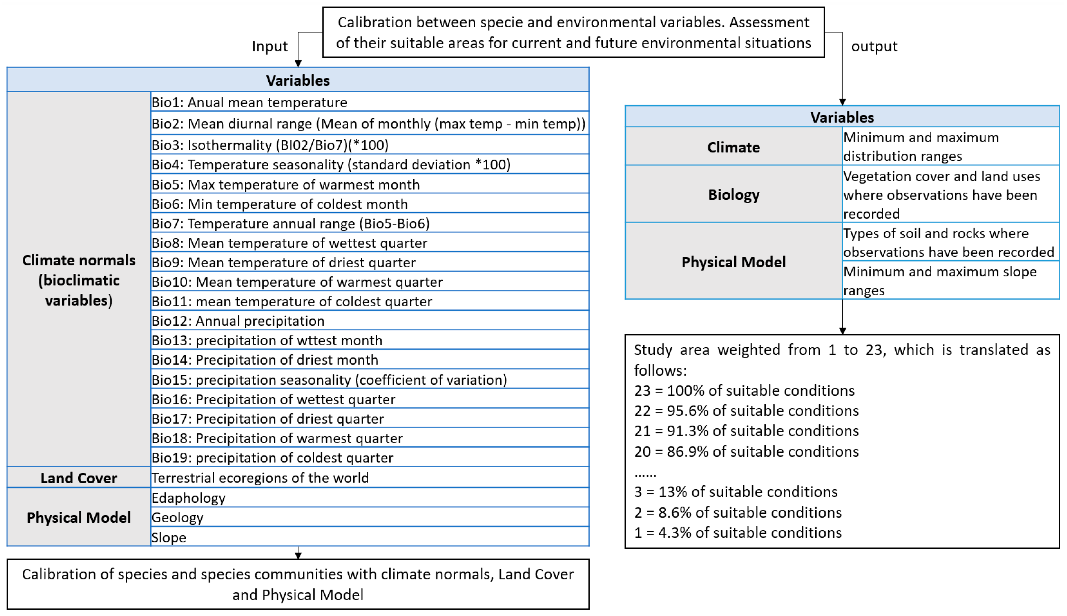
It is required to calibrate the relationships between the spatial distribution of a species (or group of species) with the spatial distribution of environmental variables that seems relevant for its development, like climate, soil types, slope, etc. This calibration represents the first step of the CDS toolbox SDM (Figure 1) which consists with the overlap of the spatial distribution of 23 environmental variables with the observations of a species. 19 are related to climatic and bioclimatic variables that are considered as relevant for the development and survival of species.

The other 4 environmental variables are related to the land use and vegetation type in which the species are observed, the type of soil, and rocks that are relevant for their ecology and the range of slope where species can be observed.

The CDS toolbox SDM does not formulate any assumption on the relationship between a species with its environment: it just considers the occurrence of the species on the values or category of each variable. In this process, each variable has the same weight in order to avoid conjectural assumptions. Like other SDM [1], the accuracy of the calibration belongs to the spatial resolution and the amount of observations and measures. The result of this first step is the identification of the range of variable values that are considered significant in order to ensure species development and survival. In another terms, this step allows establishing the ecological niche of a species. The 19 selected climatic variables are related to temperature and precipitation statistics that give a synthetic description of climatic envelop of species and can also be considered as limiting factors [22]. Temperature plays a role on plant lethality: temperatures that are too low slow down or stop the growth of plants. For example, the frost causes a mechanical action on plant cells, resulting in the formation of ice crystals which destroy cell walls. The frost also causes water loss, which leads to desiccation of certain organs. In contrast, high temperatures have an effect on the evaporation of water reserves contained in the soil and generate excessive leaf transpiration causing water stress (evapotranspiration phenomenon). Depending on its duration and intensity, it can be lethal for non-adapted or poorly adapted plants. Scorching episodes, such as the one that occurred in France and Europe in 2003, resulted in increased mortality of plants [23,24].

In this frame, we give more importance to climatic variables because they influence largely the survival of plants especially for areas where climatic gradients are significant, according to the spatial distribution of their observations and the spatial distribution of the potential suitable areas for their development. Appendix A provides a statistical description (min, max, mean, standard deviation) of the quantitative variables and the description of the classes of nominal variables.

The second step is the identification of potential suitable areas for the species survival and development according to current or future environmental situations. In our approach, we perform the two assessments (baseline and future environmental contexts) in order to identify the potential trends (increase, decrease, stability) of the spatial distribution of suitable areas for species, community of species, or landscape units.

The calculation is based on the finding of favorable conditions on a territory. In this step, the algorithm looks for the pixels where the reference conditions are the same as the one observed for species. The algorithm selects the pixels that have the same categories of nominal variables (land use, vegetation cover, edaphology, geology) and the pixels that fall in the range of quantitative variables (temperature, precipitation, slope). However, in order to take into account the uncertainty of finding similar environmental conditions for the species and their capacity to adapt to the environmental changes, the model considers 3 ecological situations:

• The species or community of species adapt slightly to the new environmental conditions and they select the areas where the conditions are closest to the optimum of reference with a contraction of the populations or the community;
• The species or community of species adapts drastically to the new environmental conditions and they can remain in the same areas;
• The species or community of species are not able to adapt to changes and disappears locally.

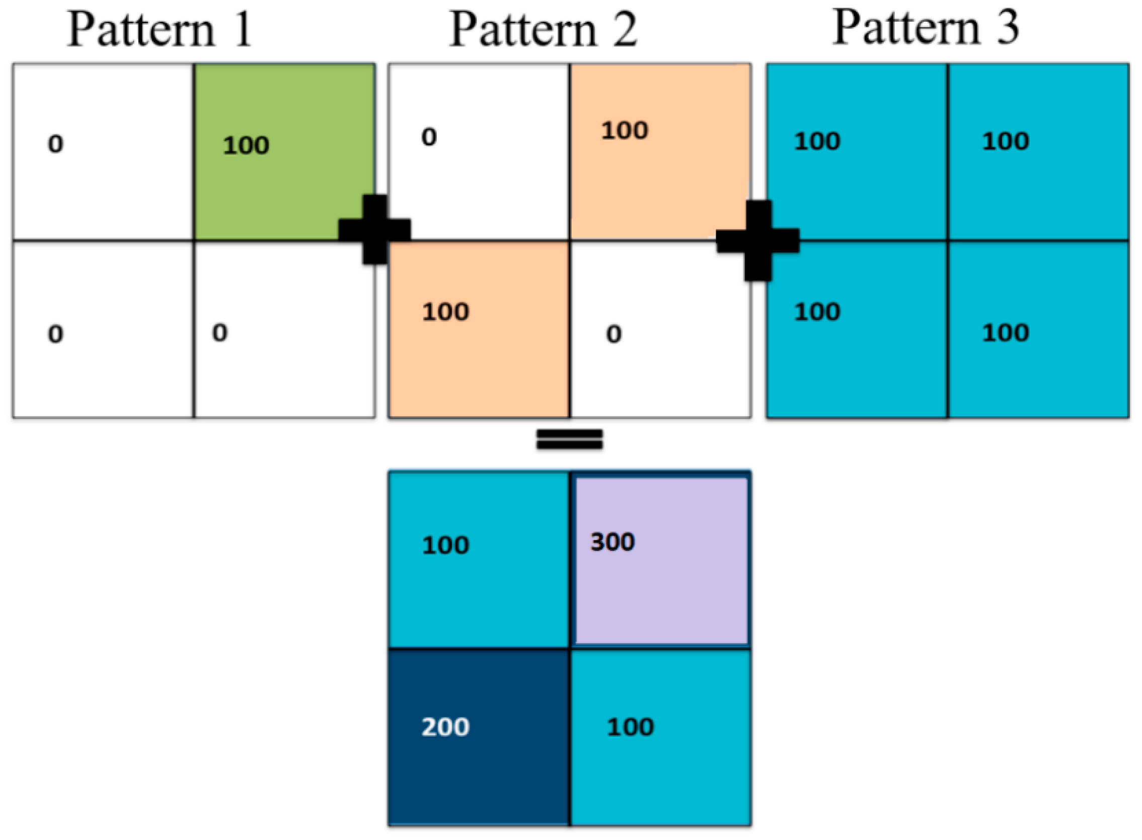
Thus, the algorithm uses a linear equation in which each of the 23 variables is summed in order to calculate the level of suitability of each area for the ecological niche of species or community of species. This parameter, named “Potential Ecological Distribution” (PED), is given by the following expression:

Potential Ecological Distribution = Variable 1 + Variable 2…+ Variable n…+ Variable 23

(1)

Figure 2 shows a hypothetical example of the application of the algorithm on four pixels of a territory and with only three variables (pattern 1 = maximum temperature, pattern 2 = minimum temperature, and pattern 3 = precipitations). For pattern 1, there is only one pixel with a value corresponding to the ecological niche of a species. For pattern 2, there are two pixels with a favorable value for the development of a species, and for pattern 3, all four pixels have a suitable value. Then, the algorithm calculates the sum of each value of variables for each pixel. The result shows that 1 pixel has the best suitability (amount = 300), another has an average level of suitability (amount = 200) and two pixels have a low level of suitability (amount = 100).

This step allows identifying the level of environmental similarity of each part of a territory that will support the decision process for ecosystems and biological resource management. This activity is related to different categories of stakeholders and decision-makers at local, regional, and national levels like Ministers of Ecology and Agriculture, Mayors and public authorities, farmers, forest managers, policy makers, protected areas administrators, supply chain supervisors, etc.

In the CDS toolbox SDM, the algorithm carries out this calculation for each pixel of a particular territory according to the 23 variables taken into account for defining the ecological niche of a species or a community of species. This process is applied for baseline and future environmental conditions especially the climatic ones based on the IPCC scenarios. The result allows identifying trends of species spatial dynamics and can help support decisions in order to manage potential changes in ecosystem services.

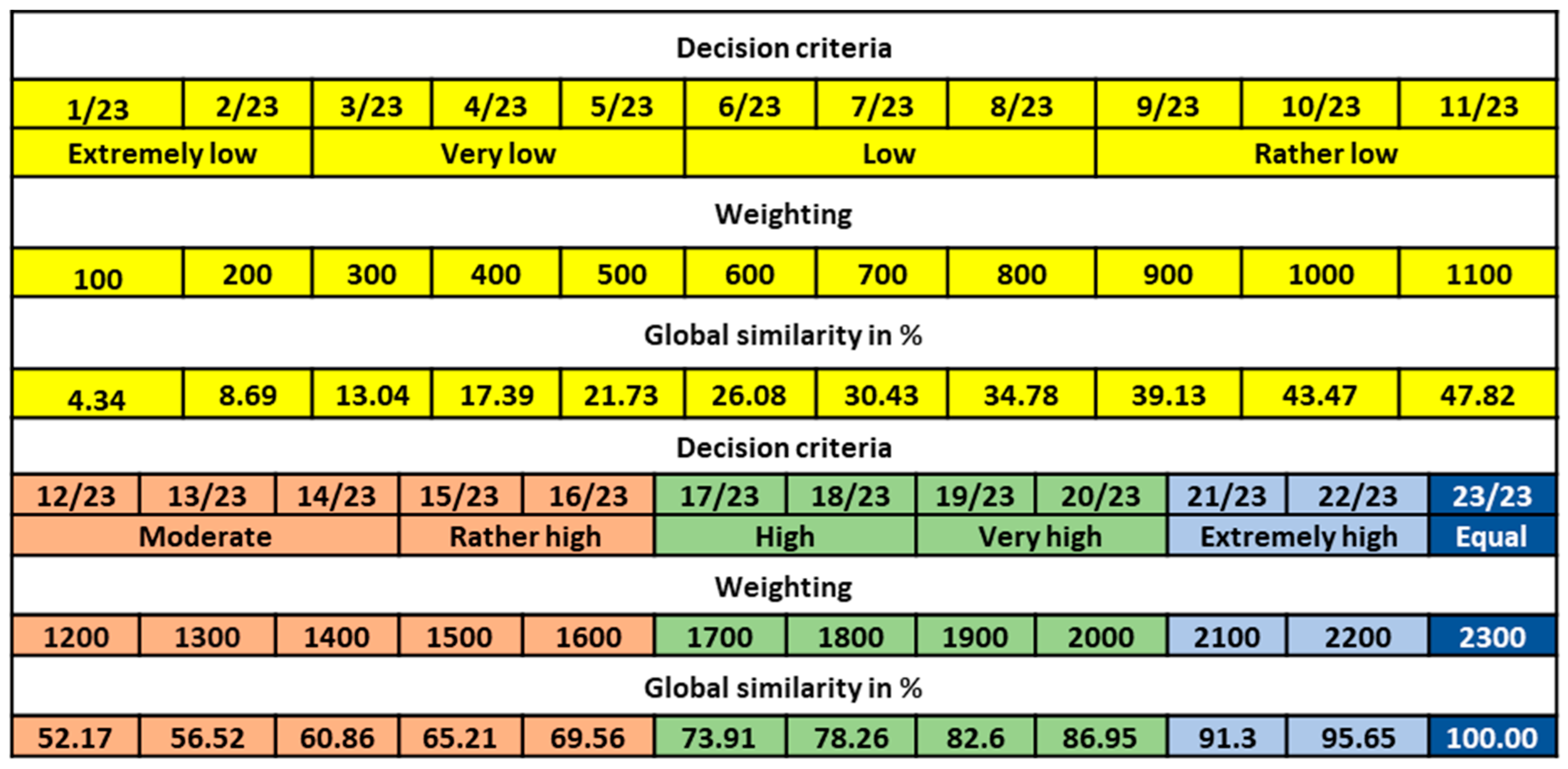
According to [25], we present, in Figure 3, the three modalities that contribute to the decision process. These decision rules are based on arithmetic and statistical procedures allowing the integration of stabilized criteria into a unique index. This index aims to help decision makers for making comparisons of alternatives of spatial distribution of species, community of species and landscape units.

In order to respect the three ecological situations mentioned previously, the interpretation of the table follows the coming logic:

• When a pixel has the 100% of global similarity (weighting = 23) it means that the pixel has 100% of suitability for species or community of species. In this area the environmental parameters correspond to the ecological niche of species or community of species (decision criteria = equal, that means equality of environmental parameters). In the case of the assessment of the potential impact of climate change on species distribution, 100% of global similarity means that species would not find problems for their life and their development.
• When a pixel has global similarity values between 82.6 and 100% (weighting = 1900, 2000, 2100 or 2200), this indicates that the environmental conditions for the species are slightly similar to their ecological niche. The potential impact of climate change should not be significant on their life and development, and the adaptation of species to the future environmental conditions should be appropriate.
• When a pixel has global similarity values between 52.17 and 82.6% (weighting between 1200 and 1800), the pixels represent an area where the species should adapt to the new environmental conditions but showing some slight periods of stress. In this case, the uncertainty for the adaption of species to the new ecological situation is more important than in the other part of the range of the global similarity values.
• Finally, when a pixel has global similarity values between 1 and 52.17% (weighting between 100 and 1200), the area can be considered as poorly suitable for the development of the species or community of species. The possibility of adaptation of species to the future environmental conditions decreases significantly.

The final result of the application of the CDS Toolbox SDM is a map showing the probability to find suitable areas for species, community of species, and landscape units.

We present hereinafter an example of the application of CDS Toolbox SDM in order to assess the spatial distribution of suitable areas for Vitis vinifera L., the common grapevine, in France. Viticulture is a key socio-economic sector in Europe. Due to the strong sensitivity of grapevines to atmospheric factors, climate change may represent an important challenge for this sector [26].

According to the CnIV (National Committee of Interprofessions of Wines), France is the leading wine and wine brandy exporter, and is the second economic sector in the trade This economic sector employs 500,000 people and it can be considered as a key sector for the economy. With 750,000 ha of grapevine crops, France represents 11% of the world surface area for wine production.

For this case study, the spatial resolution of the data is around 1 km. They come from:

• WorldClim for the 19 climatic/bioclimatic data and for the slopes (elevation layer);
• The Ecoregion Layer for the data on land cover provided by WWF (World Wildlife Fund) [27];
• GeoTypes.net for geology layer [28];
• FAO GeoNetwork (Food and Agriculture Organization of the United Nations) for the edaphology layer.

The proposed assessment aims to identify the potential problems or opportunities on such crop and, if necessary, to aware stakeholders for adapting their practices on crops, on supply chain management, and on the selection of the best areas for the cultivation of grapevine.

3. Results

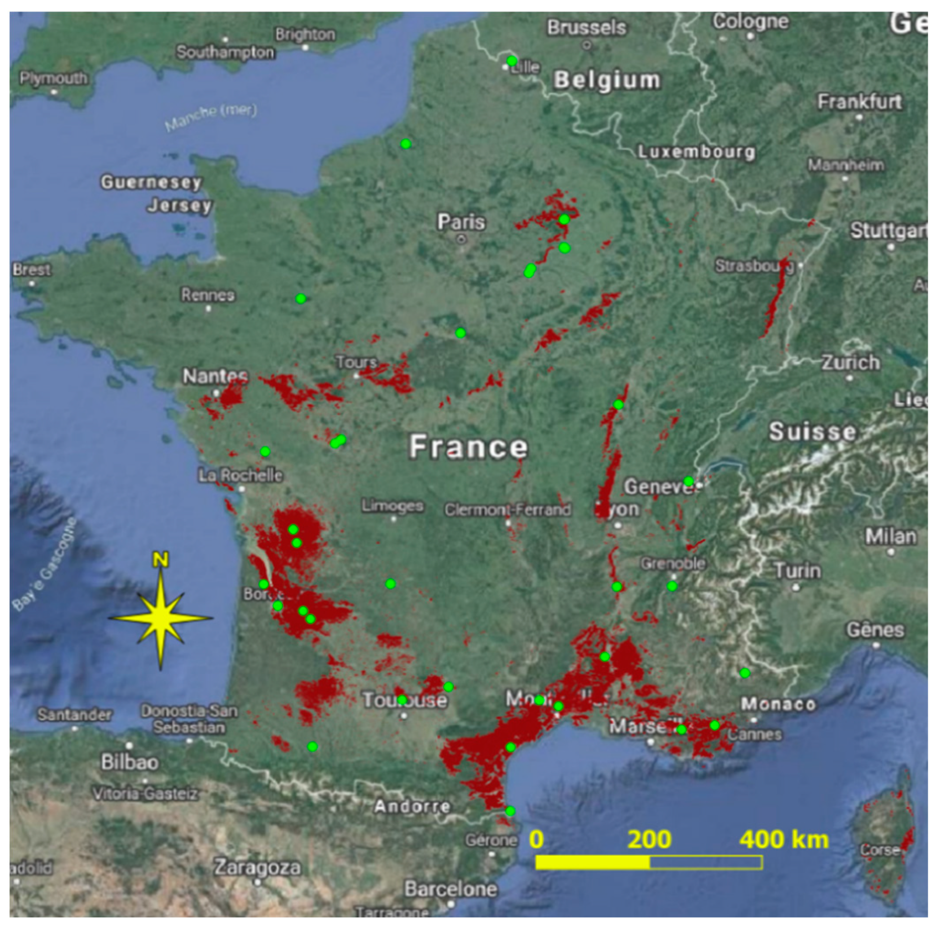
The field observations of Vitis vinifera L. in France (Figure 4) come from the iNaturalist Internet platform and they represent an amount of 35 observations. We also present the official map of grapevine crops in France (Figure 4) provided by the RGP (Parcells Geographic Register provided by the French National Geographic Institute–IGN) in 2018. All of this data is free of charge and open source.

The assessment of the suitable areas for Vitis vinifera L. has been performed for the closest climatic situation of the current period (called “baseline”) provided by the WorldClim platform and for 2050 and 2070 by the use of IPCC scenarios corresponding to two average Representative Concentration Pathway: RCP4.5 and RCP6.0. We decided to use those two scenarios because they represent moderately optimistic (RCP4.5) and moderately pessimistic (RCP6.0) scenarios of climate change according to the current and future adoption of policies and application of means dedicated to GHG (Greenhouse Gas) emissions reduction by countries, industries, and organizations.

The contributors of WorldClim dataset provided the baseline scenario that we use in our study [20] by using climatic data from 60,000 weather stations for a temporal range of 1970 to 2000. They interpolated these measures with thin-plate splines and covariates (elevation, distance to the coast, maximum and minimum temperature, cloud cover from MODIS satellite). For the scenarios of climate change, the WorldClim contributors used IPCC data for which they apply a statistical downscaling method based on interpolations [29].

These maps show the different level of probabilities that have been classified into three classes according to the Jenks Natural Break classification method [30]. This method is often used in GIS project because it allows underlying differences of different objects of a same data set in a map. This classification is based on an iterative process in order to define classes with significant differences in the values of the data.

Table 1. Ranges of the different classes of probabilities.

Classes	2050 RCP4.5		2050 RCP6.0		2070 RCP4.5		2070 RCP6.0		Baseline
1	4.34	60.86	4.34	56.52	4.34	56.52	4.34	52.17	4.34	60.86
2	60.86	82.6	56.52	82.6	56.52	78.26	52.17	78.26	60.86	86.95
3	82.6	100	82.6	100	78.26	95.65	78.26	100	86.95	100

presents the probability ranges of the different classes.

Class 1 corresponds to the low level of probabilities to find environmental conditions required for the development of a species, class 2 corresponds to the average level of probabilities, and class 3 corresponds to the high level of probabilities. The results of the model are analyzed by taking into account the different levels of probabilities to find suitable environmental conditions for the selected specie. These classes of probabilities are expressed by a colored code described below each figure.

The aim of these maps is to compare the potential spatial distribution of the suitable areas for cultivating the grapevine according to the current climatic situation and the climate change scenarios. The maps of probabilities to find suitable areas are presented on the left side of the figure while the right side of the figure represents the current probabilities to find suitable areas and the current locations of grapevine crops.

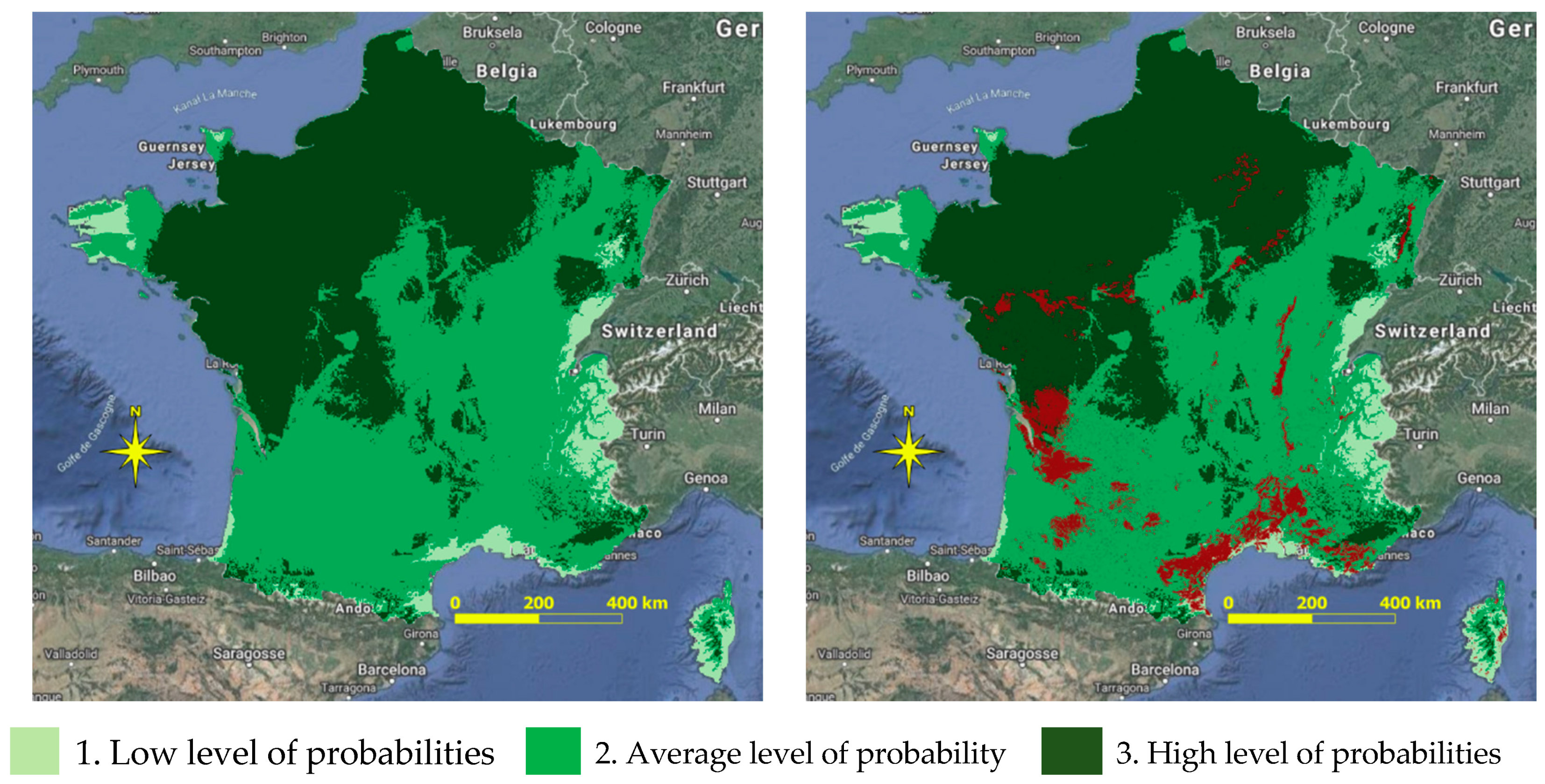
Figure 5 shows the potential suitable areas for Vitis vinifera L. in France according to the baseline climate. It also presents the location of the map of grapevine crops in order to compare its spatial distribution with the probabilities to find suitable areas.

A simple visual analysis of the maps shows that the current declared grapevine crops are mainly localized in the high probability level to find suitable areas for the development of Vitis vinifera L. The quantitative analysis of the overlap of these two information layers (

Table 2. Percentage and ha of grapevine crops in the probability classes to find suitable area.

	% of Polygons Outside of Suitable Areas	ha Outside of Suitable Areas	% of Polygons in Low Proba. Class	ha in Low Proba. Class	% of Polygons in Average Proba. Class	ha in Average Proba. Class	% of Polygons in High Proba. Class	ha in High Proba. Class
Baseline	<1	0	0	0	7	52,500	93	697,500
2050 RCP 4.5	1	7500	16	120,000	64	480,000	19	142,500
2050 RCP 6.0	1	7500	1	7500	46	345,000	52	390,000
2070 RCP 4.5	1	7500	5	37,500	85	637,500	9	67,500
2070 RCP 6.0	1	7500	1	7500	49	367,500	49	367,500

) shows that 93% of the surface of grapevine crops are located into the high level of probability to find suitable areas for this cultivation. This first result demonstrates the relevance of the model in order to assess the spatial distribution of suitable territories of this specie.

The other areas of grapevine crops (7%) are located into to average probability of occurrence of suitable areas and there are no declared crops in the low probability class. Only 0.1% of the crops’ surfaces are in areas that do not present any probability of occurrence. For the other results relating to the assessment for the future (2050 and 2070), they present a value of 1% of grapevine crops in areas without any probability to find suitable areas.

The analysis of Table 2 underlines a significant potential decrease of cultivated crops in the areas of high probably of suitable areas, according to the baseline scenario: this decrease would be of 555,000 ha for 2050 RCP4.5 scenario, 307,500 ha for 2050 RCP6.0 scenario, 630,000 ha for 2070 RCP4.5 and 330,000 ha for 2070 RCP6.0.

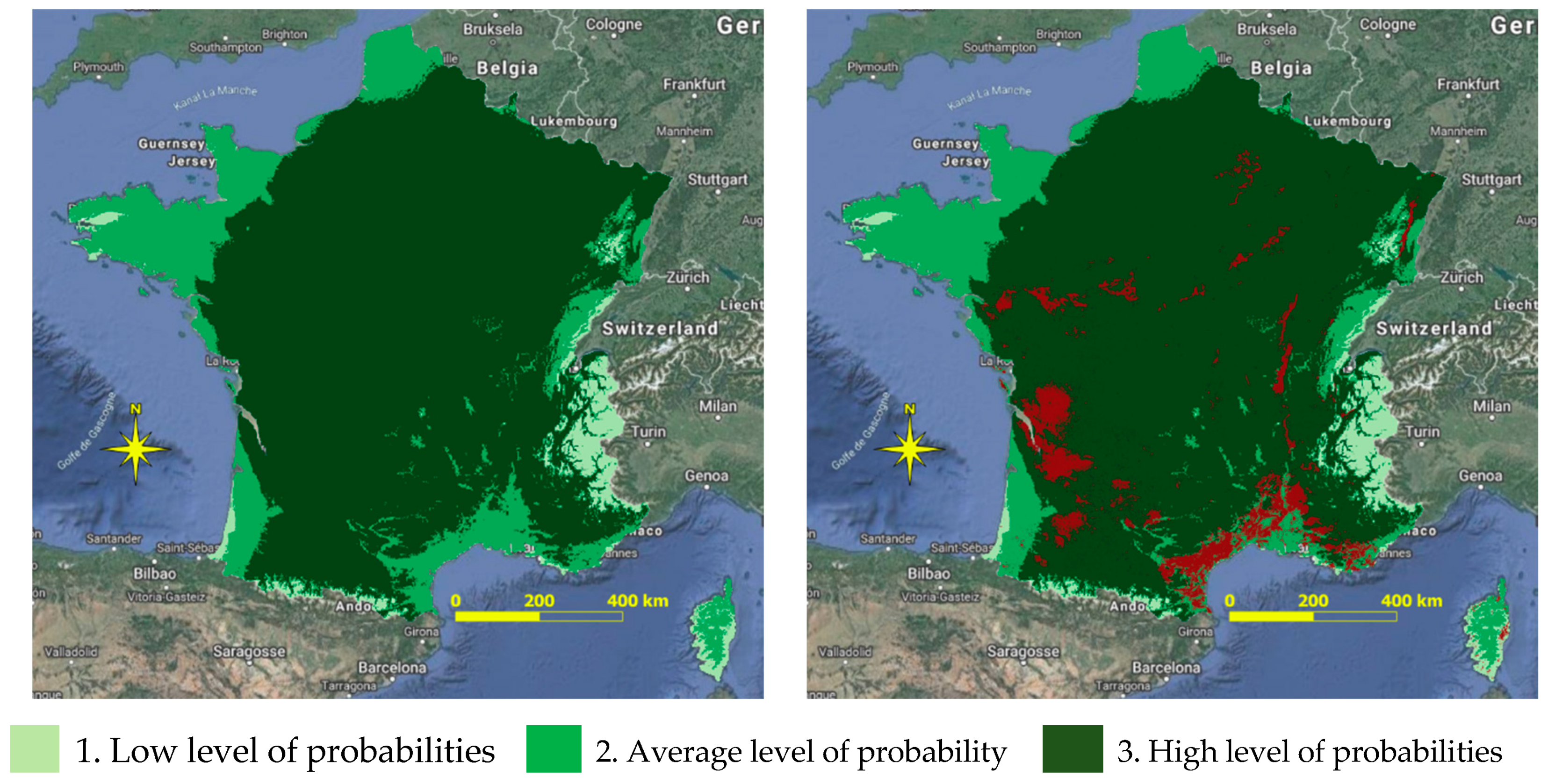
According to these first results, it is possible to compare the baseline situation with the potential future situations. The simulation of the potential impact of RCP4.5 climate scenario for 2050 (Figure 6) on the spatial distribution of suitable areas for Vitis vinifera L. shows a significant decrease of high level of probabilities on the French territory.

The comparison with the current grapevine crops (Table 2) shows that only 19% of the crops should be in the high level of probability to find suitable areas, 64% in the average level, and 16% in the low level.

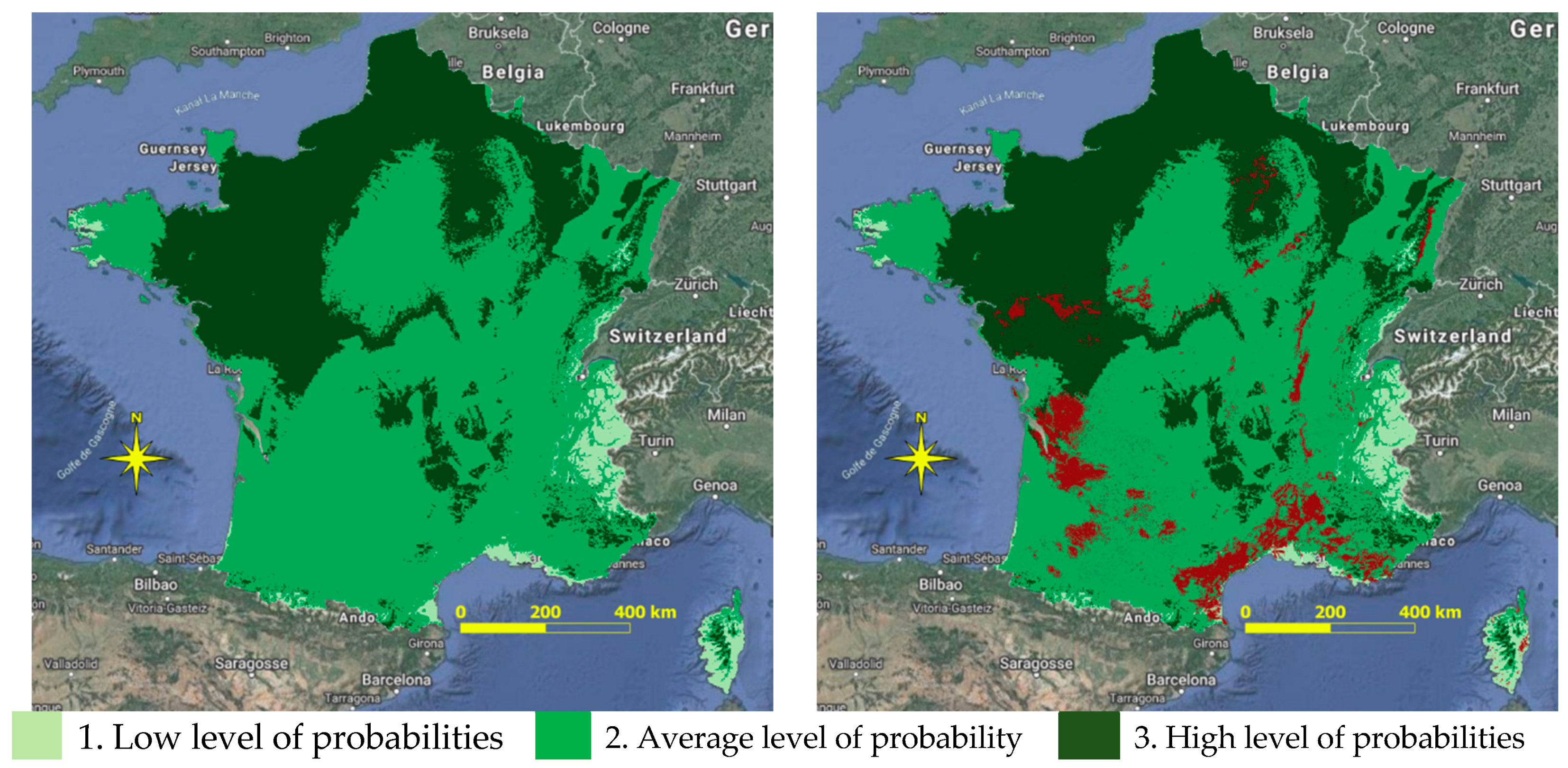
At the opposite of the previous result, the simulation of the potential impact of RCP6.0 climate scenario for 2050 on the spatial distribution of suitable areas for Vitis vinifera L. (Figure 7) presents a less contrasted situation. The comparison with the current grapevine crops (Table 2) shows that 52% of the crops should be in the high level of probability to find suitable areas, 46% in the average level, and only 1% in the low level.

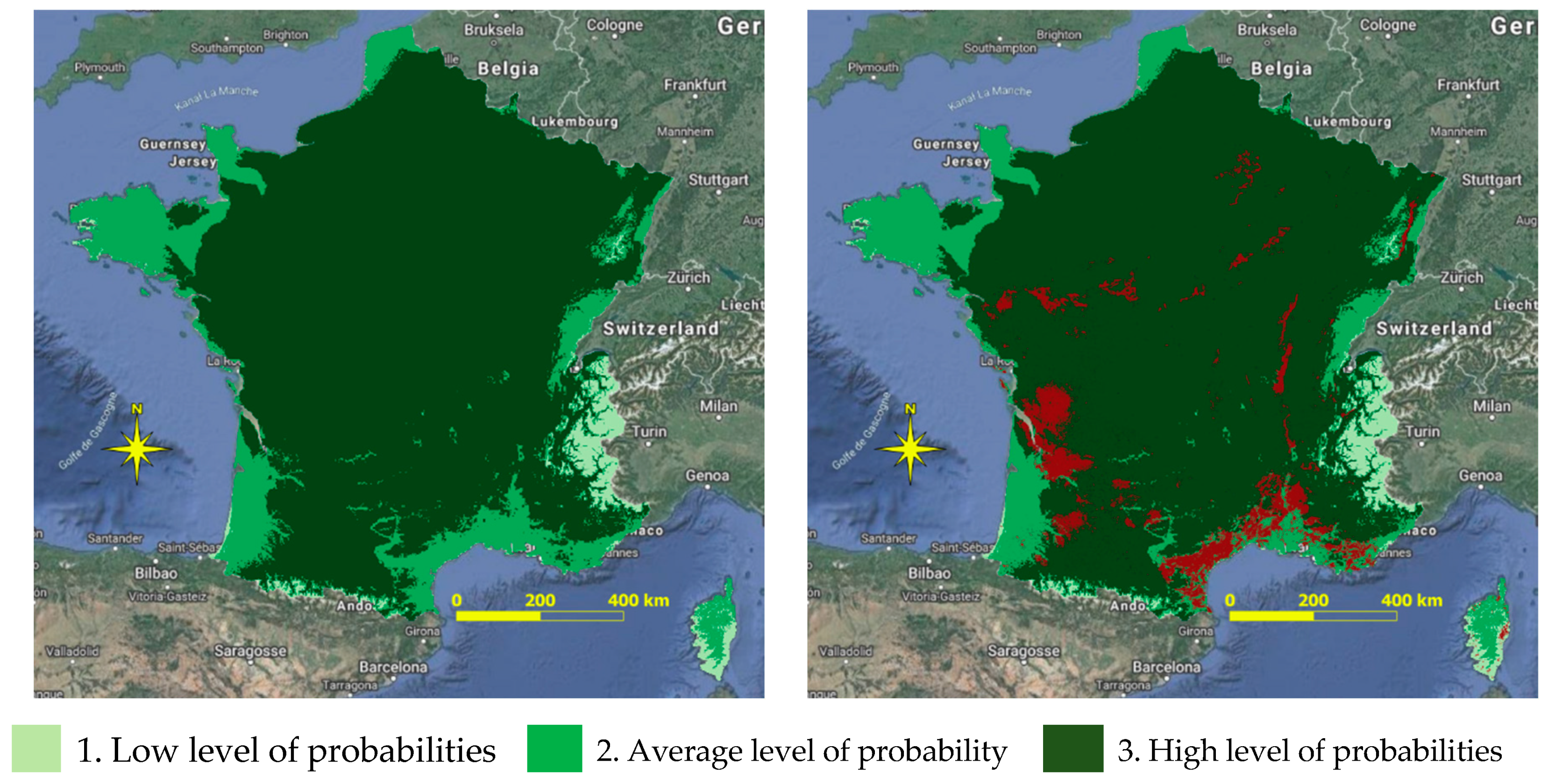
The modeling of the potential spatial distribution of suitable areas for Vitis vinifera L. in 2070 with RCP4.5 scenario (Figure 8) confirms the decrease of high probability class on the French territory. The comparison with the current crops areas shows that they should be located mainly in average probability class (85%) for this scenario (Table 2). The rest of the spatial distribution should correspond to 9% in high probability class and 5% in the low probability class.

The assessment of potential suitable areas for 2070 according to RCP6.0 scenario (Figure 9) presents a potential equivalent spatial distribution of grapevine crops of 49% for high and average classes of probability. Only 1% of current cultivations should be located in the lowest probability class.

The results presented in

Table 3. Average altitude of polygons into the different probability classes according to baseline and future climate scenarios.

Title Climate Scenarios	Avg. Alti. (m) Outside of Suitable Areas	Avg. Alti. (m) in Low Proba. Class	Avg. Alti. (m) in Average Proba. Class	Avg. Alti. (m) in High Proba. Class
Baseline	390	1306	421	233
2050 RCP 4.5	387	934	386	204
2050 RCP 6.0	384	1408	269	297
2070 RCP 4.5	387	1207	342	231
2070 RCP 6.0	384	1601	302	297

are related to the statistical distribution of the average altitude in each class of probability and according to the different climatic situations (baseline, 2050 and 2070).

This table highlights that the areas with a high level of probability to find suitable areas for grapevine crops should be located in higher altitudes than the current ones for scenario RCP6.0 in 2050 and 2070. For scenario RCP4.5, there could be a global decrease of average altitudes for 2050 and 2070 according to the baseline situation. This decrease should be significant with the low and average classes of probability.

The analysis of the whole results underlines that the current location of grapevine crops are mainly situated in high level probability class (93%) but, according to the potential impact of climate change, these areas should become less favorable to its cultivation towards 2050 and 2070, even if the RCP4.5 and RCP6.0 scenarios show contrasted future situations. The variation of the surface located in the high probability class would decrease from 41% to 84% of the amount of the current areas situated in this class which would represent an amount between 307,500 ha and 630,000 ha where grapevines would face some perturbations on its growth and its mortality rate.

The results also show that RCP4.5 scenario would have a more drastic impact on the spatial distribution of suitable areas for grapevine than RCP6.0 scenario for both 2050 and 2070 periods in France because most of the crops would be situated in average and low probability classes with RCP4.5 scenario.

4. Discussion

The application of CDS Toolbox SDM on the potential suitability of grapevine crops in France shows two main ecological and biogeographical mechanisms.

The first one is the selection pressure that leads to the contraction of the spatial distribution of species. This appears when the suitable areas are very few (global similarity values between 1 and 52.17%) like it is for class 1. In this case, species cannot adapt or may face very difficult problems to adapt to the future environmental conditions. The result is a decrease of the surface they previously colonized.

The second one is the environmental pressure on the phenotypic plasticity that can lead or not to the expansion of the areas colonized by the species or community of species. This process is complex because there are different ways of expression of the phenotypic plasticity. One of these possibilities is the contraction of the distribution area of species that correspond to the resistance of new environmental conditions. This process can also generate a migration of species to other areas that are more suitable but the areas colonized remain lower than the previous ecological situation (classes 2 and 3). Another type of expression of phenotypic plasticity is the expansion of the specie in more areas than before because the environmental changes provides areas that are more suitable.

With the use of RCP4.5 scenarios for the 2050 and 2070 periods, CDS Toolbox SDM shows that climate change would have a significant negative role on the spatial distribution of suitable areas for grapevine crops. RCP4.5 scenario seems to have a more drastic impact on the spatial distribution of grapevine than RCP6.0 scenario. Nevertheless, those two scenarios also show a significant decrease of suitable areas for grapevine in 2050 and 2070 according to its current distribution. This result is coherent with the conclusions of [31], which identified that new territories should be suitable for grapevine cultivation in the northern part of France by using A1B from penultimate IPCC climate scenarios version (scenario similar to RCP6.0, [32]) with three downscaling methods (weather type—WT; Quantile-Quantile—QQ; and Anomalies—ANO) in 2050 and 2100, but without proposing a mapping method. The model developed by [32] is based on the use of annual means and standard deviation in order to calculate the climate change impact on phenology, transpiration ratio, and climatic water balance [33], using a GIS approach, also shows a potential shift of suitable areas for viniculture towards 2100 in the northern part of France. They use the penultimate IPCC scenarios B1 (scenario close to RCP2.6 scenario, the most optimistic one, [31]) and A1B with a spatial resolution of 18 km. The estimation of the potential distribution of suitable areas is based on the spatial distribution of bioclimatic variables, but without calibrating the relationships between vineyards areas and these variables.

Fraga et al. [34] present similar trends with RCP4.5 and RCP8.5 scenarios in order to show the potential impact of climate change on climatic suitability of 44 varieties of grapevine in Portugal. Their results show a potential shift of suitable areas in the northern part of Portugal and other European countries and in higher altitudes than currently. Their model is based on a spatial resolution of 1 km using the WorldClim dataset and they focus their analysis on the spatial distribution of bioclimatic indexes and their correlation with the viticultural regions of Portugal.

Moriondo et al. [35] argue that climate change would provoke a shift in the north and north-west of their current location in France, Germany, Italy, Portugal and Spain using A2 and B2 scenarios towards 2050 at 1 km of spatial resolution. They also underline the potential expansion or contraction of some suitable areas for grapevine crops according to the potential impact of climate change.

In the frame of the European CORDEX project (Coordinated Downscaling Experiment—European Domain) Cardell et al. [36] studied the evolution of 11 bioclimatic indices for 3 periods (2021–2045, 2046–2070, 2071–2095) by using RCP4.5 and RCP8.5 scenarios at 12 km of spatial resolution. Their results show that climate change would induce a shift of suitable areas for grape wine crops in Central and Northern parts of Europe like Germany, North of France, Belgium, Poland, Southern England and Czech Republic due to better temperatures around 2050. Our study presents similar conclusions but with a more accurate spatial resolution (1 km) at the scale of the French territory.

In Italy, Caffarra and Eccel [37], by using A2 (scenario similar to RCP6.0, IPCC 2013) and B2 (scenario similar to RCP8.5, [31]) IPCC scenarios from the penultimate version of climatic assessment, mention that mountain areas at an elevation of around 1000 m in the region of Trentino (Italian Alps) would be suitable for the cultivation of grapevine due climate change towards 2100. In our model, the potential development of the grapevine in mountains is more nuanced, especially for the territories situated in high levels of probability to find suitable conditions. According to RCP6.0 in 2050 and 2070, there could be a potential increase of the average altitude but only around 300m. The areas situated around 1000 m mainly match with low probability class to find suitable environmental conditions for the cultivation of grapevine.

However, CDS Toolbox SDM also underlines that the potential impact of climate change may be less significant than the other studies suppose. This is particularly the case by the use of RCP6.0 scenario for 2050 and 2070. In this case, it seems that the future climate conditions related to RCP6.0 scenario would be more favorable for the grapevine crops than the one related to RCP4.5 scenario. These results show the ability of CDS Toolbox SDM to render the bioclimatic dimension of the relationship between the species and the climatic variables, which is a relevant aspect in order to help decision-makers establish their strategy to make their activities resilient to climate change.

5. Conclusions

CDS Toolbox SDM has been developed in order to help decision-makers adapt their strategy and activities concerning the biological resources (biodiversity, agriculture, landscape, etc.) to the potential impacts of climate change. The aim of this model is to support a prospective approach that can be considered as a key process to ensure territorial resilience.

The application of CDS Toolbox SDM on the viniculture in France has shown the capability of the model to take into account the different potential impacts of climate change on the spatial distribution of suitable areas for grapevine crops according to the scenarios RCP4.5 and RCP6.0 for 2050 and 2070 periods. These results can contribute to define practical actions in order to adapt viniculture to climate change. For example, some of these actions can be related to developing irrigation infrastructures and techniques as suggested by [31]. Another strategy could be based on the diversification of cultivars. In that frame, [38] demonstrated that the use of 11 grapevine cultivars may help to reduce the potential losses of suitable areas by a half (for a 2 °C scenario) or by a third (for a 4 °C) for 2100. Finally, CDS Toolbox SDM can be used in order to identify the territories that are and would still be suitable for grapevine crops towards 2050 and 2070 in order to plan the development of wine supply chain in regions where this cultivation has not been developed or only slightly so.

As an improvement of CDS Toolbox SDM, we plan to add a climatic downscaling module allowing the use of climate change scenarios at very high spatial resolution (75 m) in order to provide the results at parcels scale. Because Morales-Castilla et al. [38] underlines that climate change since the 2000s affected the production of wine, especially when drought occurs during the growing season in summer, we also plan to combine our approach with the use of other climate based indexes like the Net Primary Productivity (NPP). This index is able to assess the potential productivity of vineyard through the next decades and its potential impact on the expected grapevine harvest. As suggested by [39,40], the implementation of the Huglin index, used at high spatial resolution, could also be helpful in order to map the potential evolution of the thermal requirements of grape varieties and the potential sugar content of grapes, this last parameter being relevant for wine producers.