Comparison of Backscatter Coefficient at 1064 nm from CALIPSO and Ground–Based Ceilometers over Coastal and Non–Coastal Regions


Abstract
:1. Introduction
2. Instruments and Data
2.1. CALIOP
2.2. Jenoptik CHM15K Lidar Ceilometer
3. Study Sites
3.1. Coastal Area: Mace Head (MH)
3.2. Non–Coastal Area: Harzgerode (DWD)
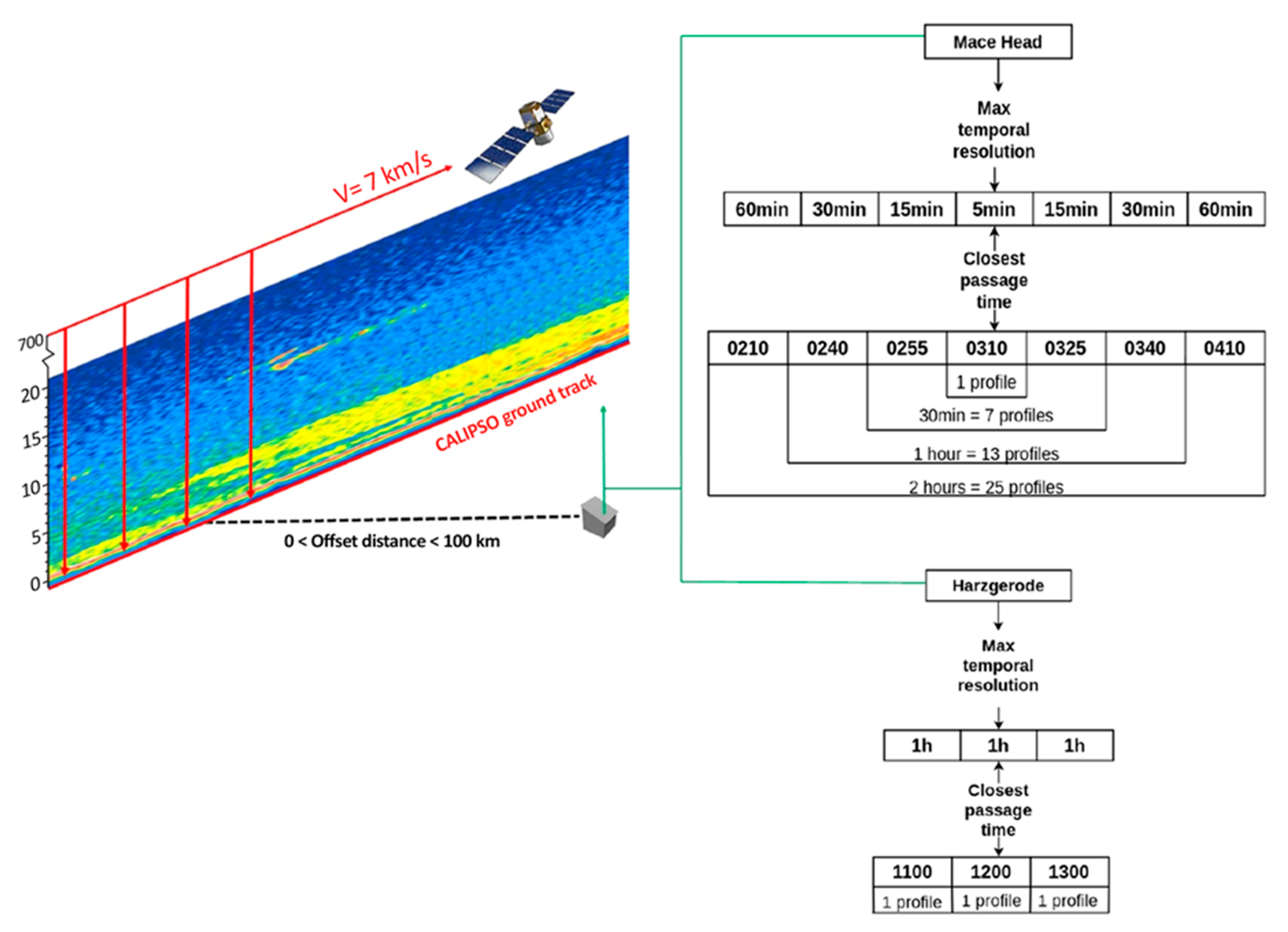
4. Comparison Methodology
5. Results and Discussion
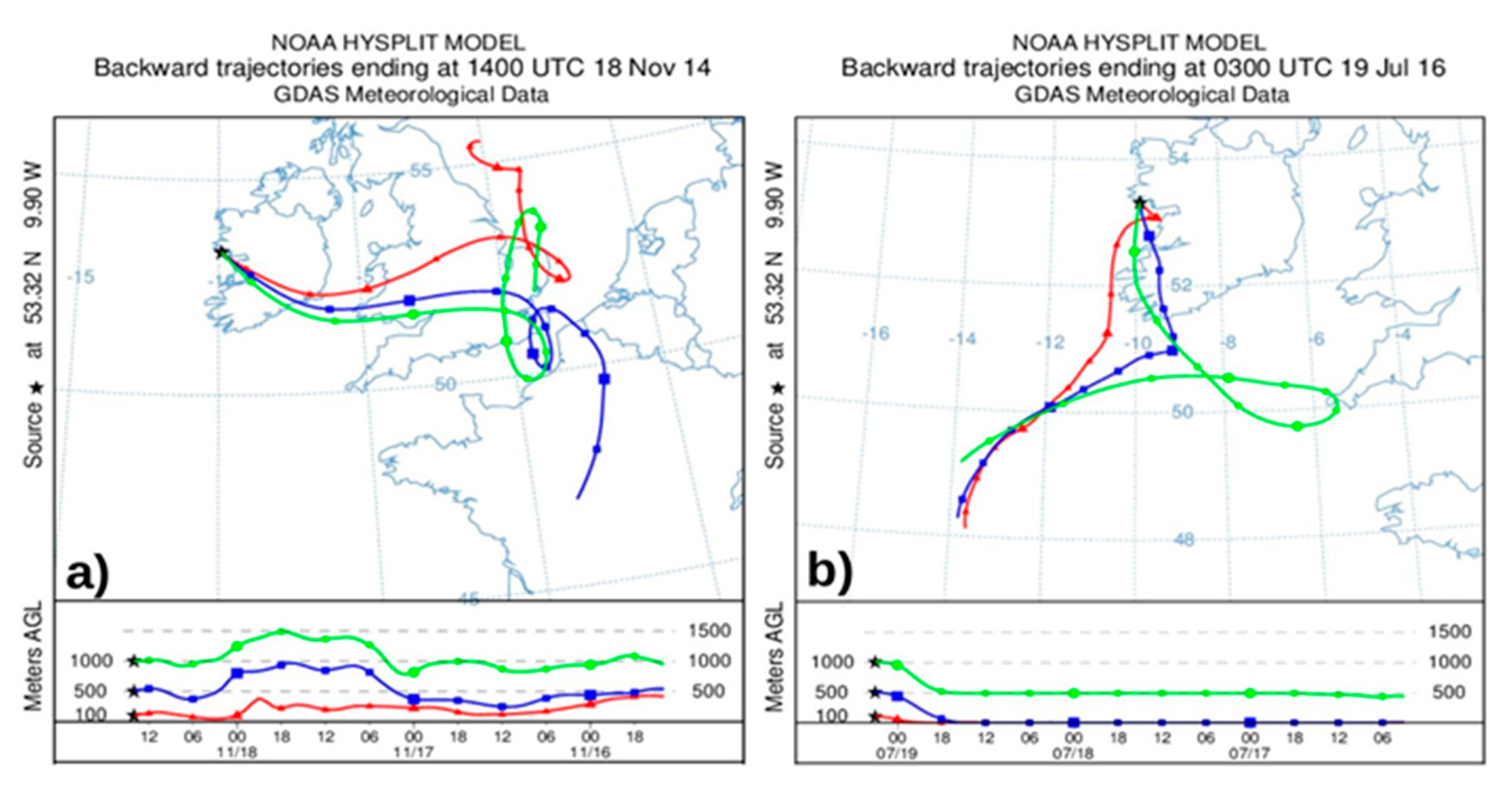
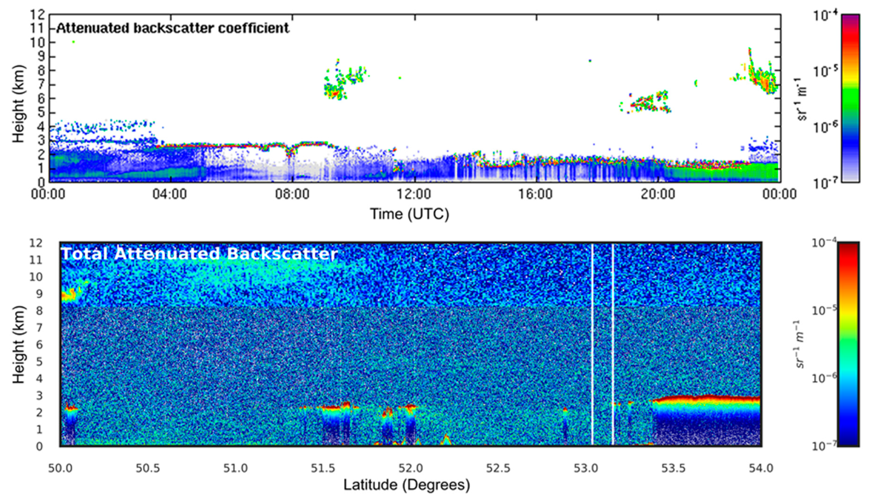
5.1. Case Studies
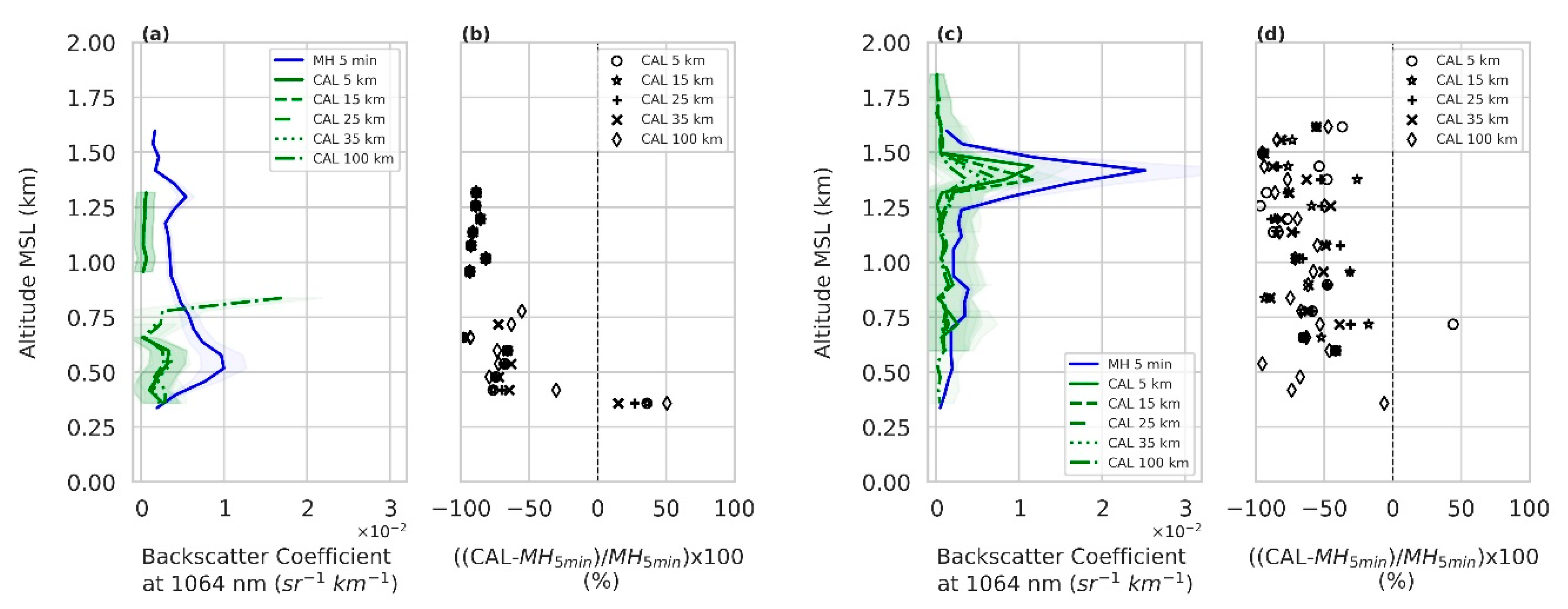
5.1.1. Coastal Region–Mace Head
5.1.2. Non–Coastal Region—Harzgerode–DWD
5.2. Long–Term Comparison
6. Summary and Conclusions
Author Contributions
Funding
Acknowledgments
Conflicts of Interest
Appendix A. Statistical Terms
Appendix A.1. The Mean Bias (MB)
Appendix A.2. The Mean Percentage Difference
Appendix A.3. The Correlation Coefficient (R)
Appendix A.4. Factor of Exceedance (FoE)
Appendix B. Mean Backscatter Coefficient Values for the Case Studies
Appendix B.1. Mace Head

| Along–Track Average | Mean Backscatter Coefficient (sr−1km−1) | |
|---|---|---|
| 2018/11/14 | 2019/7/16 | |
| 5 km | 1 × 10⁻³ ± 1 × 10⁻³ | 2 × 10⁻³ ± 3 × 10⁻³ |
| 15 km | 1 × 10⁻³ ± 1 × 10⁻³ | 2 × 10⁻³ ± 3 × 10⁻³ |
| 25 km | 1 × 10⁻³ ± 1 × 10⁻³ | 1 × 10⁻³ ± 2 × 10⁻³ |
| 35 km | 1 × 10⁻³ ± 1 × 10⁻³ | 1 × 10⁻³ ± 1 × 10⁻³ |
| 100 km | 2 × 10⁻³ ± 4 × 10⁻³ | 1 × 10⁻³ ± 1 × 10⁻³ |
| MH 5 min | 4 × 10⁻³ ± 2 × 10⁻³ | 5 × 10⁻³ ± 6 × 10⁻³ |
Appendix B.2. Harzgerode—DWD
| Along–Track Average | Mean Backscatter Coefficient ( sr−1km−1) | |
|---|---|---|
| 06/08/14 | 04/05/16 | |
| 5 km | 1 × 10⁻³ ± 1 × 10⁻³ | 1 × 10⁻³ ± 6 × 10⁻⁴ |
| 15 km | 1 × 10⁻³ ± 1 × 10⁻³ | 1 × 10⁻³ ± 6 × 10⁻⁴ |
| 25 km | 1 × 10⁻³ ± 1 × 10⁻³ | 1 × 10⁻³ ± 6 × 10⁻⁴ |
| 35 km | 1 × 10⁻³ ± 1 × 10⁻³ | 1 × 10⁻³ ± 6 × 10⁻⁴ |
| 100 km | 1 × 10⁻³ ± 1 × 10⁻³ | 1 × 10⁻³ ± 6 × 10⁻⁴ |
| DWD 60 min | 4 × 10⁻⁴ ± 4 × 10⁻⁴ | 1 × 10⁻³ ± 2 × 10⁻⁴ |
Appendix C. Mace Head Case Studies with Different Temporal Resolution


| Temporal Resolution 5 min | 2018/11/14 | 2019/7/16 | ||||||
|---|---|---|---|---|---|---|---|---|
| MPD (%) | R | p Value | MB (sr−1km−1) | MPD (%) | R | p Value | MB (sr−1km−1) | |
| 5 km | −75 ± 35 | 0.60 | 0.03 | −4 × 10⁻³ | −58 ± 37 | 0.87 | 0 | −4 × 10⁻³ |
| 15 km | −75 ± 35 | 0.60 | 0.03 | −4 × 10⁻³ | −61 ± 23 | 0.72 | 0 | −4 × 10⁻³ |
| 25 km | −75 ± 32 | 0.62 | 0.02 | −4 × 10⁻³ | −63 ± 20 | 0.71 | 0 | −4 × 10⁻³ |
| 35 km | −75 ± 28 | 0.68 | 0.01 | −4 × 10⁻³ | −66 ± 17 | 0.70 | 0 | −4 × 10⁻³ |
| 100 km | −49 ± 89 | 0.06 | 0.82 | −3 × 10⁻³ | −67 ± 20 | 0.58 | 0 | −4 × 10⁻³ |
| Temporal Resolution 30 min | 2018/11/14 | 2019/7/16 | ||||||
|---|---|---|---|---|---|---|---|---|
| MPD (%) | R | p Value | MB (sr−1km−1) | MPD (%) | R | p Value | MB (sr−1km−1) | |
| 5 km | −72 ± 40 | 0.38 | 0.2 | −4 × 10⁻³ | −62 ± 37 | 0.84 | 0 | −4 × 10⁻³ |
| 15 km | −72 ± 40 | 0.38 | 0.2 | −4 × 10⁻³ | −66 ± 26 | 0.69 | 0 | −3 × 10⁻³ |
| 25 km | −73 ± 37 | 0.4 | 0.18 | −4 × 10⁻³ | −68 ± 23 | 0.67 | 0 | −4 × 10⁻³ |
| 35 km | −72 ± 33 | 0.47 | 0.09 | −4 × 10⁻³ | −71 ± 19 | 0.67 | 0 | −4 × 10⁻³ |
| 100 km | −46 ± 91 | −0.01 | 0.98 | −3 × 10⁻³ | −71 ± 22 | 0.55 | 0 | −4 × 10⁻³ |
| Temporal Resolution 60 min | 2018/11/14 | 2019/7/16 | ||||||
|---|---|---|---|---|---|---|---|---|
| MPD (%) | R | p Value | MB (sr−1km−1) | MPD (%) | R | p Value | MB (sr−1km−1) | |
| 5 km | −73 ± 39 | 0.24 | 0.43 | −4 × 10⁻³ | −65 ± 34 | 0.76 | 0 | −4 × 10⁻³ |
| 15 km | −73 ± 39 | 0.24 | 0.43 | −4 × 10⁻³ | −71 ± 25 | 0.63 | 0 | −4 × 10⁻³ |
| 25 km | −74 ± 37 | 0.25 | 0.41 | −4 × 10⁻³ | −73 ± 20 | 0.6 | 0 | −4 × 10⁻³ |
| 35 km | −74 ± 33 | 0.32 | 0.26 | −4 × 10⁻³ | −75 ± 17 | 0.59 | 0 | −4 × 10⁻³ |
| 100 km | −52 ± 78 | 0.03 | 0.9 | −3 × 10⁻³ | −75 ± 22 | 0.49 | 0.01 | −4 × 10⁻³ |
Appendix D. Mean Backscatter Coefficient Values for Long–Term Comparison
| Along–Track Average | Mean Backscatter Coefficient( sr−1km−1) | |
|---|---|---|
| DAYTIME | NIGHTTIME | |
| 5 km | 2 × 10⁻³ ± 1 × 10⁻³ | 2 × 10⁻³ ± 1 × 10⁻³ |
| 15 km | 2 × 10⁻³ ± 1 × 10⁻³ | 2 × 10⁻³ ± 1 × 10⁻³ |
| 25 km | 2 × 10⁻³ ± 1 × 10⁻³ | 2 × 10⁻³ ± 1 × 10⁻³ |
| 35 km | 2 × 10⁻³ ± 1 × 10⁻³ | 1 × 10⁻³ ± 1 × 10⁻³ |
| 100 km | 2 × 10⁻³ ± 1 × 10⁻³ | 2 × 10⁻³ ± 1 × 10⁻³ |
| MH 60 min | 5 × 10⁻⁴ ± 2 × 10⁻⁴ | 7 × 10⁻⁴ ± 3 × 10⁻⁴ |
| Along–Track Average | Mean Backscatter Coefficient ( sr−1km−1) | |
|---|---|---|
| DAYTIME | NIGHTTIME | |
| 5 km | 1 × 10⁻³ ± 4 × 10⁻⁴ | 1 × 10⁻³ ± 1 × 10⁻³ |
| 15 km | 1 × 10⁻³ ± 4 × 10⁻⁴ | 1 × 10⁻³ ± 1 × 10⁻³ |
| 25 km | 1 × 10⁻³ ± 4 × 10⁻⁴ | 2 × 10⁻³ ± 1 × 10⁻³ |
| 35 km | 1 × 10⁻³ ± 4 × 10⁻⁴ | 2 × 10⁻³ ± 2 × 10⁻³ |
| 100 km | 1 × 10⁻³ ± 3 × 10⁻⁴ | 2 × 10⁻³ ± 2 × 10⁻³ |
| DWD 60 min | 9 × 10⁻⁴ ± 2 × 10⁻⁴ | 4 × 10⁻⁴ ± 1 × 10⁻⁴ |
References
- Haywood, J.M.; Francis, P.N.; Dubovik, O.; Glew, M.; Holben, B. Comparison of aerosol size distributions, radiative properties, and optical depths determined by aircraft observations and Sun photometers during SAFARI 2000. J. Geophys. Res. Space Phys. 2003, 108. [Google Scholar] [CrossRef]
- Forster, P.; Ramaswamy, V.; Artaxo, P.; Berntsen, T.; Betts, R.; Fahey, D.W.; Haywood, J.; Lean, J.; Lowe, D.C.; Myhre, G.; et al. Changes in Atmospheric Constituents and in Radiative Forcing; Chapter 2. In Climate Change 2007: The Physical Science Basis; Cambridge University Press: Cambridge, UK, 2007. [Google Scholar]
- Burton, S.P.; Ferrare, R.A.; Hostetler, C.A.; Hair, J.W.; Kittaka, C.; Vaughan, M.A.; Obland, M.D.; Rogers, R.R.; Cook, A.L.; Harper, D.B.; et al. Using airborne high spectral resolution lidar data to evaluate combined active plus passive retrievals of aerosol extinction profiles. J. Geophys. Res. Space Phys. 2010, 115. [Google Scholar] [CrossRef] [Green Version]
- Kim, S.W.; Berthier, S.; Chazette, P.; Raut, J.C.; Dulac, F.; Yoon, S.C. Validation of aerosol and cloud layer structures from the space–borne lidar CALIOP using Seoul National University ground–based lidar. Atmos. Chem. Phys. 2007, 7, 11207–11222. [Google Scholar] [CrossRef] [Green Version]
- Winker, D.M.; Pelon, J.; Coakley, J.A.; Ackerman, S.A.; Charlson, R.J.; Colarco, P.R.; Flamant, P.; Fu, Q.; Hoff, R.M.; Kittaka, C.; et al. The CALIPSO Mission. Bull. Am. Meteorol. Soc. 2010, 91, 1211–1230. [Google Scholar] [CrossRef]
- Wandinger, U.; Freudenthaler, V.; Baars, H.; Amodeo, A.; Engelmann, R.; Mattis, I.; Groß, S.; Pappalardo, G.; Giunta, A.; D’Amico, G.; et al. EARLINET instrument intercomparison campaigns: Overview on strategy and results; Discussion Paper 26. Atmos. Meas. Tech. 2016, 9, 1001–1023. [Google Scholar] [CrossRef] [Green Version]
- Pappalardo, G.; Wandinger, U.; Mona, L.; Hiebsch, A.; Mattis, I.; Amodeo, A.; Ansmann, A.; Seifert, P.; Linné, H.; Apituley, A.; et al. EARLINET correlative measurements for CALIPSO: First intercomparison results. J. Geophys. Res. Space Phys. 2010, 115. [Google Scholar] [CrossRef] [Green Version]
- Welton, E.J.C. The Micro–Pulse Lidar Network (MPL–Net). In Proceedings of the XXI International Laser Radar Conference, Quebec City, QC, Canada, 8–12 July 2002. [Google Scholar]
- Guerrero–Rascado, J.L.; Landulfo, E.; Antuña, J.C.; Barbosa, H.M.J.; Barja, B.; Bastidas, Á.E.; Bedoya, A.E.; Da Costa, R.F.; Estevan, R.; Forno, R.; et al. Latin American Lidar Network (LALINET) for aerosol research: Diagnosis on network instrumentation. J. Atmos. Solar Terr. Phys. 2016, 138, 112–120. [Google Scholar] [CrossRef]
- Sugimoto, N.; Nishizawa, T.; Shimizu, A.; Jin, Y. The Asian Dust and Aerosol Lidar Observation Network (AD–Net). In Light, Energy and the Environment; Paper EW2A.1; The Optical Society: Washington, DC, USA, 2016. [Google Scholar]
- Mamouri, R.E.; Amiridis, V.; Papayannis, A.; Giannakaki, E.; Tsaknakis, G.; Balis, D.S. Validation of CALIPSO space–borne–derived attenuated backscatter coefficient profiles using a ground–based lidar in Athens, Greece. Atmos. Meas. Tech. 2009, 2, 513–522. [Google Scholar] [CrossRef] [Green Version]
- Powell, K.A.; Hostetler, C.A.; Vaughan, M.A.; Lee, K.–P.; Trepte, C.R.; Rogers, R.R.; Winker, D.M.; Liu, Z.; Kuehn, R.E.; Hunt, W.H. CALIPSO lidar calibration algorithms. Part I: Nighttime 532–nm parallel channel and 532–nm perpendicular channel. J. Atmos. Oceanic Technol. 2009, 26, 2015–2033. [Google Scholar] [CrossRef]
- Winker, D.M.; Vaughan, M.; Omar, A.; Hu, Y.; Powell, K.A.; Liu, Z.; Hunt, W.H.; Young, S.A. Overview of the CALIPSO Mission and CALIOP Data Processing Algorithms. J. Atmos. Ocean. Technol. 2009, 26, 2310–2323. [Google Scholar] [CrossRef]
- Grigas, T.; Hervo, M.; Gimmestad, G.; Forrister, H.; Schneider, P.; Preißler, J.; Tarrason, L.; O’Dowd, C. CALIOP near–real–time backscatter products compared to EARLINET data. Atmos. Chem. Phys. 2015, 15, 12179–12191. [Google Scholar] [CrossRef] [Green Version]
- Martucci, G.; Milroy, C.; O’Dowd, C.D. Detection of Cloud–Base Height Using Jenoptik CHM15K and Vaisala CL31 Ceilometers. J. Atmos. Ocean. Technol. 2010, 27, 305–318. [Google Scholar] [CrossRef]
- Mona, L.; Pappalardo, G.; Amodeo, A.; D’Amico, G.; Madonna, F.; Boselli, A.; Giunta, A.; Russo, F.; Cuomo, V. One year of CNR–IMAA multi–wavelength Raman lidar measurements in coincidence with CALIPSO overpasses: Level 1 products comparison. Atmos. Chem. Phys. 2009, 9, 7213–7228. [Google Scholar] [CrossRef] [Green Version]
- Hu, Y.; Stamnes, K.; Vaughan, M.; Pelon, J.; Weimer, C.; Wu, D.; Cisewski, M.; Sun, W.; Yang, P.; Lin, B.; et al. Sea surface wind speed estimation from space–based lidar measurements. Atmos. Chem. Phys. 2008, 9. [Google Scholar] [CrossRef] [Green Version]
- Tesche, M.; Wandinger, U.; Ansmann, A.; Althausen, D.; Muller, D.; Omar, A.H. Ground-based validation of CALIPSO observations of dust and smoke in the Cape Verde region. J. Geophys. Res. Atmos. 2013, 118, 2889–2902. [Google Scholar] [CrossRef]
- Wu, Y.; Cordero, L.; Gross, B.; Moshary, F.; Ahmed, S. Assessment of CALIPSO attenuated backscatter and aerosol retrievals with a combined ground–based multi–wavelength lidar and sunphotometer measurement. Atmos. Environ. 2014, 84, 44–53. [Google Scholar] [CrossRef]
- Binietoglou, I.; Amodeo, A.; D’Amico, G.; Giunta, A.; Madonna, F.; Mona, L.; Pappalardo, G. Examination of possible synergy between lidar and ceilometer for the monitoring of atmospheric aerosols. In Lidar Technologies, Techniques, and Measurements for Atmospheric Remote Sensing VII; International Society for Optics and Photonics: Washington, DC, USA, 2011; Volume 8182, p. 818209. [Google Scholar]
- Pappalardo, G.; Mona, L.; Damico, G.; Wandinger, U.; Adam, M.; Amodeo, A.; Ansmann, A.; Apituley, A.; Alados–Arboledas, L.; Balis, D.; et al. Four–dimensional distribution of the 2010 Eyjafjallajökull volcanic cloud over Europe observed by EARLINET. Atmos. Chem. Phys. 2013, 13, 4429–4450. [Google Scholar] [CrossRef] [Green Version]
- Wiegner, M.; Madonna, F.; Binietoglou, I.; Forkel, R.; Gasteiger, J.; Geiß, A.; Pappalardo, G.; Schäfer, K.; Thomas, W. What is the benefit of ceilometers for aerosol remote sensing? An answer from EARLINET. Atmos. Meas. Tech. 2014, 19, 1979–1997. [Google Scholar] [CrossRef] [Green Version]
- Wiegner, M.; Geis, A. Aerosol profiling with the Jenoptik ceilometer CHM15kx. Atmos. Meas. Tech. 2012, 5, 1953–1964. [Google Scholar] [CrossRef] [Green Version]
- Heese, B.; Flentje, H.; Althausen, D.; Ansmann, A.; Frey, S. Ceilometer lidar comparison: Backscatter coefficient retrieval and signal–to–noise ratio determination. Atmos. Meas. Tech. 2010, 3, 1763–1770. [Google Scholar] [CrossRef] [Green Version]
- Caicedo, V.; Rappenglück, B.; Lefer, B.; Morris, G.; Toledo, D.; Delgado, R. Comparison of aerosol lidar retrieval methods for boundary layer height detection using ceilometer aerosol backscatter data. Atmos. Meas. Tech. 2017, 10, 1609–1622. [Google Scholar] [CrossRef] [Green Version]
- Kotthaus, S.; Grimmond, C.S.B. Atmospheric boundary-layer characteristics from ceilometer measurements. Part 1: A new method to track mixed layer height and classify clouds. Q. J. R. Meteorol. Soc. 2018, 144, 1525–1538. [Google Scholar] [CrossRef] [Green Version]
- Tsaknakis, G.; Papayannis, A.; Kokkalis, P.; Amiridis, V.; Kambezidis, H.D.; Mamouri, R.E.; Georgoussis, G.; Avdikos, G. Inter–comparison of lidar and ceilometer retrievals for aerosol and Planetary Boundary Layer profiling over Athens, Greece. Atmos. Meas. Tech. 2011, 4, 1261–1273. [Google Scholar] [CrossRef] [Green Version]
- Flentje, H.; Claude, H.; Elste, T.; Gilge, S.; Kohler, U.; Plass–Dülmer, C.; Steinbrecht, W.; Thomas, W.; Werner, A.; Fricke, W. The Eyjafjallajökull eruption in April 2010—Detection of volcanic plume using in–situ measurements, ozone sondes and lidar–ceilometer profiles. Atmos. Chem. Phys. 2010, 10, 10085–10092. [Google Scholar] [CrossRef] [Green Version]
- Flentje, H.; Heese, B.; Reichardt, J.; Thomas, W. Aerosol profiling using the ceilometer network of the German Meteorological Service. Atmos. Meas. Tech. Discuss. 2010, 3, 3643–3673. [Google Scholar] [CrossRef]
- Gasteiger, J.; Groß, S.; Freudenthaler, V.; Wiegner, M. Volcanic ash from Iceland over Munich: Mass concentration retrieved from ground–based remote sensing measurements. Atmos. Chem. Phys. 2010, 10, 26705–26750. [Google Scholar] [CrossRef]
- Hervo, M.; Haeffelin, M.; Hopkin, E.; Kotthaus, S.; Ruefenacht, R.; Thomas, W.; de Haij, M.; Mortier, A.; Laffineur, Q.; Itsvan, S.; et al. Smoke Long range transport: Monitoring with the new European automatic Lidar and ceilometer network: E–PROFILE. In Proceedings of the AGU Fall Meeting, Washington, DC, USA, 10–14 December 2018; p. 23. [Google Scholar]
- Kambezidis, H.D.; Paliatsos, A.G.; Kappos, N.; Kasselouri, B. A Case of African Dust Transport over Athens Captured by a Ceilometer. In Proceedings of the Advances in Meteorology, Climatology and Atmospheric Physics; Helmis, C.G., Nastos, P.T., Eds.; Springer: Berlin/Heidelberg, Germany, 2013; pp. 1011–1018. [Google Scholar]
- Cazorla, A.; Casquero–Vera, J.A.; Román, R.; Guerrero–Rascado, J.L.; Toledano, C.; Cachorro, V.E.; Orza, J.A.G.; Cancillo, M.L.; Serrano, A.; Titos, G.; et al. Near–real–time processing of a ceilometer network assisted with sun–photometer data: Monitoring a dust outbreak over the Iberian Peninsula. Atmos. Chem. Phys. 2017, 17, 11861–11876. [Google Scholar] [CrossRef] [Green Version]
- Lee, J.; Hong, J.W.; Lee, K.; Hong, J.; Velasco, E.; Lim, Y.J.; Lee, J.B.; Nam, K.; Park, J. Ceilometer Monitoring of Boundary–Layer Height and its Application in Evaluating the Dilution Effect on Air Pollution. Bound. Layer Meteorol. 2019, 172, 435–455. [Google Scholar] [CrossRef] [Green Version]
- Li, S.; Joseph, E.; Min, Q.; Yin, B.; Sakai, R.; Payne, M.K. Remote sensing of PM2.5 during cloudy and nighttime periods using ceilometer backscatter. Atmos. Meas. Tech. 2017, 10, 2093–2104. [Google Scholar] [CrossRef] [Green Version]
- Warren, E.; Charlton–Perez, C.; Kotthaus, S.; Lean, H.; Ballard, S.; Hopkin, E.; Grimmond, C. Evaluation of forward–modelled attenuated backscatter using an urban ceilometer network in London under clear–sky conditions. Atmos. Environ. 2018, 191, 532–547. [Google Scholar] [CrossRef]
- Kolláth, K.; Kolláth, Z. On the feasibility of using ceilometer backscatter profile as input data for skyglow simulation. J. Quant. Spectrosc. Radiat. Transf. 2020, 253, 107158. [Google Scholar] [CrossRef]
- Alexander, S.P.; Protat, A. Cloud Properties Observed from the Surface and by Satellite at the Northern Edge of the Southern Ocean. J. Geophys. Res. Atmos. 2018, 123, 443–456. [Google Scholar] [CrossRef]
- Snels, M.; Scoccione, A.; Di Liberto, L.; Colao, F.; Pitts, M.; Poole, L.; Deshler, T.; Cairo, F.; Cagnazzo, C.; Fierli, F. Comparison of Antarctic polar stratospheric cloud observations by ground–based and space–borne lidar and relevance for chemistry–climate models. Atmos. Chem. Phys. 2019, 19, 955–972. [Google Scholar] [CrossRef] [Green Version]
- Vaughan, M.A.; Garnier, A.; Josset, D.; Avery, M.; Lee, K.P.; Liu, Z.; Hunt, W.; Pelon, J.; Hu, Y.; Burton, S.; et al. CALIPSO lidar calibration at 1064 nm: Version 4 algorithm. Atmos. Meas. Tech. 2019, 12, 51–82. [Google Scholar] [CrossRef] [Green Version]
- Chen, B.; Huang, J.; Minnis, P.; Hu, Y.; Yi, Y.; Liu, Z.; Zhang, D.; Wang, X. Detection of dust aerosol by combining CALIPSO active lidar and passive IIR measurements. Atmos. Chem. Phys. 2010, 10, 4241–4251. [Google Scholar] [CrossRef] [Green Version]
- Hunt, W.H.; Winker, D.M.; Vaughan, M.A.; Powell, K.A.; Lucker, P.L.; Weimer, C. CALIPSO Lidar Description and Performance Assessment. J. Atmos. Ocean. Technol. 2009, 26, 1214–1228. [Google Scholar] [CrossRef]
- NASA Langley ASDC (2010), CALIPSO Data Quality Statements: Summary Statement for the Release of the CALIPSO Lidar Level 2 Cloud and Aerosol Profile Products Version 3.01, May 2010, Report, Hampton, Va. Available online: http://www–calipso.larc.nasa.gov/resources/calipso_users_guide/data_quality (accessed on 22 March 2020).
- Kim, M.H.; Omar, A.H.; Tackett, J.L.; Vaughan, M.A.; Winker, D.M.; Trepte, C.R.; Hu, Y.; Liu, Z.; Poole, L.R.; Pitts, M.C.; et al. The CALIPSO version 4 automated aerosol classification and lidar ratio selection algorithm. Atmos. Meas. Tech. 2018, 11, 6107–6135. [Google Scholar] [CrossRef] [PubMed] [Green Version]
- Hervo, M.; Poltera, Y.; Haefele, A. An empirical method to correct for temperature–dependent variations in the overlap function of CHM15k ceilometers. Atmos. Meas. Tech. 2016, 9, 2947–2959. [Google Scholar] [CrossRef] [Green Version]
- Preißler, J.; Martucci, G.; Saponaro, G.; Ovadnevaite, J.; Vaishya, A.; Kolmonen, P.; Ceburnis, D.; Sogacheva, L.; de Leeuw, G.; O’Dowd, C.D. Six years of surface remote sensing of stratiform warm clouds in marine and continental air over Mace Head, Ireland. J. Geophys. Res. Atmos. 2016, 121, 14538. [Google Scholar] [CrossRef] [Green Version]
- Odowd, C.D.; Ceburnis, D.; Ovadnevaite, J.; Vaishya, A.; Rinaldi, M.; Facchini, M.C. Do anthropogenic, continental or coastal aerosol sources impact on a marine aerosol signature at Mace Head? Atmos. Chem. Phys. 2014, 14, 10687–10704. [Google Scholar] [CrossRef] [Green Version]
- O’Connor, T.; Jennings, S.; O’Dowd, C.D. Highlights of fifty years of atmospheric aerosol research at Mace Head. Atmos. Res. 2008, 90, 338–355. [Google Scholar] [CrossRef]
- O’Dowd, C.D.; Hämeri, K.; Väkevä, M.; Aalto, P.; Becker, E.; Hansson, H.; Harrison, R.M.; Berresheim, H.; Kleefeld, C.; Geever, M.; et al. Coastal new particle formation: Environmental conditions and aerosol physicochemical characteristics during nucleation bursts. J. Geophys. Res. Space Phys. 2002, 107, 12. [Google Scholar] [CrossRef] [Green Version]
- O’Dowd, C.D.; Varghese, S.; Martin, D.; Flanagan, R.; McKinstry, A.; Ceburnis, D.; Ovadnevaite, J.; Martucci, G.; Bialek, J.; Monahan, C.; et al. The Eyjafjallajökull ash plume—Part 2: Simulating ash cloud dispersion with REMOTE. Atmos. Environ. 2012, 48, 143–151. [Google Scholar] [CrossRef]
- Ovadnevaite, J.; Ceburnis, D.; Plauskaite–Sukiene, K.; Modini, R.L.; Dupuy, R.; Rimselyte, I.; Ramonet, M.; Kvietkus, K.; Ristovski, Z.; Berresheim, H.; et al. Volcanic sulphate and arctic dust plumes over the North Atlantic Ocean. Atmos. Environ. 2009, 43, 4968–4974. [Google Scholar] [CrossRef] [Green Version]
- Jennings, S.; Geever, M.; McGovern, F.; Francis, J.; Spain, T.; Donaghy, T. Microphysical and physico–chemical characterization of atmospheric marine and continental aerosol at mace head. Atmos. Environ. 1997, 31, 2795–2808. [Google Scholar] [CrossRef]
- Rüfenacht, R.; Hervo, M.; Mona, L.; Papagiannopoulos, N.; Rosoldi, M.; D’Amico, G.; Mattis, I.; Cazorla, A.; Alados–Arboledas, L.; Luis, J.; et al. The European network of automatic lidars and ceilometers E–PROFILE: Validation through EARLINET/ACTRIS measurements and potential for satellite cal/val. 1. Geophys. Res. Abstr. 2019, 21, 1. [Google Scholar]
- Tao, Z.; McCormick, M.; Wu, D. A comparison method for spaceborne and ground–based lidar and its application to the CALIPSO lidar. Appl. Phys. A 2008, 91, 639–644. [Google Scholar] [CrossRef]
- Gimmestad, G.; Forrister, H.; Grigas, T.; O’Dowd, C.D. Comparisons of aerosol backscatter using satellite and ground lidars: Implications for calibrating and validating spaceborne lidar. Sci. Rep. 2017, 7, 42337. [Google Scholar] [CrossRef] [PubMed] [Green Version]
- Mosca, S.; Graziani, G.; Klug, W.; Bellasio, R.; Bianconi, R. A statistical methodology for the evaluation of long–range dispersion models. Atmos. Environ. 1998, 32, 4307–4324. [Google Scholar] [CrossRef]
- Stein, A.F.; Draxler, R.R.; Rolph, G.D.; Stunder, B.J.B.; Cohen, M.D.; Ngan, F. NOAA’s HYSPLIT Atmospheric Transport and Dispersion Modeling System. Bull. Am. Meteorol. Soc. 2015, 96, 2059–2077. [Google Scholar] [CrossRef]


| Temporal Resolution 5 min | 2018/11/14 | 2019/7/16 | ||||||
|---|---|---|---|---|---|---|---|---|
| MPD (%) | R | p Value | MB (sr−1km−1) | MPD (%) | R | p Value | MB (sr−1km−1) | |
| 5 km | −75 ± 35 | 0.6 | 0.03 | −4 × 10⁻³ | −58 ± 37 | 0.87 | 0 | −4 × 10⁻³ |
| 15 km | −75 ± 35 | 0.6 | 0.03 | −4 × 10⁻³ | −61 ± 23 | 0.72 | 0 | −4 × 10⁻³ |
| 25 km | −75 ± 32 | 0.62 | 0.02 | −4 × 10⁻³ | −63 ± 20 | 0.71 | 0 | −4 × 10⁻³ |
| 35 km | −75 ± 28 | 0.68 | 0.01 | −4 × 10⁻³ | −66 ± 17 | 0.7 | 0 | −4 × 10⁻³ |
| 100 km | −49 ± 89 | 0.06 | 0.82 | −3 × 10⁻³ | −67 ± 20 | 0.58 | 0 | −4 × 10⁻³ |
| Temporal Resolution 60 min | 2006/8/14 | 2004/5/16 | ||||||
|---|---|---|---|---|---|---|---|---|
| MPD (%) | R | p Value | MB (sr−1km−1) | MPD (%) | R | p Value | MB (sr−1km−1) | |
| 5 km | 298 ± 420 | 0.65 | 0 | 0.4 × 10⁻³ | 2 ± 54 | 0.57 | 0.03 | 0.05 × 10⁻³ |
| 15 km | 298 ± 420 | 0.65 | 0 | 0.4 × 10⁻³ | 2 ± 54 | 0.57 | 0.03 | 0.05 × 10⁻³ |
| 25 km | 286 ± 370 | 0.66 | 0 | 0.4 × 10⁻³ | 2 ± 54 | 0.57 | 0.03 | 0.05 × 10⁻³ |
| 35 km | 270 ± 334 | 0.65 | 0 | 0.3 × 10⁻³ | 2 ± 54 | 0.57 | 0.03 | 0.05 × 10⁻³ |
| 100 km | 281 ± 316 | 0.6 | 0 | 0.3 × 10⁻³ | 7 ± 55 | 0.44 | 0.09 | 0.08 × 10⁻³ |
| Temporal Resolution 60 min | DAYTIME 6 Cases | NIGHTTIME 9 Cases | ||
|---|---|---|---|---|
| MPD (%) | MB (sr−1km−1) | MPD (%) | MB (sr−1km−1) | |
| 5 km | −50 ± 41 | −2 × 10⁻³ | −80 ± 17 | −4 × 10⁻³ |
| 15 km | −50 ± 40 | −2 × 10⁻³ | −81 ± 16 | −4 × 10⁻³ |
| 25 km | −50 ± 40 | −2 × 10⁻³ | −80 ± 16 | −4 × 10⁻³ |
| 35 km | −50 ± 39 | −2 × 10⁻³ | −80 ± 17 | −4 × 10⁻³ |
| 100 km | −49 ± 42 | −2 × 10⁻³ | −73 ± 27 | −4 × 10⁻³ |
| Temporal Resolution 60 min | DAYTIME 4 Cases | NIGHTTIME 24 Cases | ||
|---|---|---|---|---|
| MPD (%) | MB (sr−1km−1) | MPD (%) | MB (sr−1km−1) | |
| 5 km | 68 ± 157 | 2 × 10⁻³ | 216 ± 206 | 4 × 10⁻³ |
| 15 km | 68 ± 157 | 2 × 10⁻³ | 274 ± 359 | 3 × 10⁻³ |
| 25 km | 68 ± 154 | 2 × 10⁻³ | 318 ± 337 | 3 × 10⁻³ |
| 35 km | 67 ± 150 | 2 × 10⁻³ | 343 ± 368 | 2 × 10⁻³ |
| 100 km | 63 ± 142 | 2 × 10⁻³ | 445 ± 563 | 2 × 10⁻³ |
| Total Cases | −0.5 < FoE < 0. 0 | FoE = 0.0 | 0.0 < FoE < 0.5 | FoE Mean | MB < 0 | MB = 0 | MB > 0 | MB Mean (sr−1km−1) |
|---|---|---|---|---|---|---|---|---|
| Mace Head | 93% | 0% | 7% | −0.28 | 80% | 13% | 7% | −3 × 10⁻³ |
| Harzgerode–DWD | 0% | 0% | 100% | 0.34 | 0% | 32% | 68% | 3 × 10⁻³ |
Publisher’s Note: MDPI stays neutral with regard to jurisdictional claims in published maps and institutional affiliations. |
© 2020 by the authors. Licensee MDPI, Basel, Switzerland. This article is an open access article distributed under the terms and conditions of the Creative Commons Attribution (CC BY) license (http://creativecommons.org/licenses/by/4.0/).
Share and Cite
Baroni, T.; Pandey, P.; Preissler, J.; Gimmestad, G.; O’Dowd, C. Comparison of Backscatter Coefficient at 1064 nm from CALIPSO and Ground–Based Ceilometers over Coastal and Non–Coastal Regions. Atmosphere 2020, 11, 1190. https://doi.org/10.3390/atmos11111190
Baroni T, Pandey P, Preissler J, Gimmestad G, O’Dowd C. Comparison of Backscatter Coefficient at 1064 nm from CALIPSO and Ground–Based Ceilometers over Coastal and Non–Coastal Regions. Atmosphere. 2020; 11(11):1190. https://doi.org/10.3390/atmos11111190
Chicago/Turabian StyleBaroni, Thaize, Praveen Pandey, Jana Preissler, Gary Gimmestad, and Colin O’Dowd. 2020. "Comparison of Backscatter Coefficient at 1064 nm from CALIPSO and Ground–Based Ceilometers over Coastal and Non–Coastal Regions" Atmosphere 11, no. 11: 1190. https://doi.org/10.3390/atmos11111190
APA StyleBaroni, T., Pandey, P., Preissler, J., Gimmestad, G., & O’Dowd, C. (2020). Comparison of Backscatter Coefficient at 1064 nm from CALIPSO and Ground–Based Ceilometers over Coastal and Non–Coastal Regions. Atmosphere, 11(11), 1190. https://doi.org/10.3390/atmos11111190