Article

Analysis of the ETNA 2015 Eruption Using WRF–Chem Model and Satellite Observations

1
Institute of Atmospheric Sciences and Climate (ISAC), National Research Council (CNR), Unit of Lecce, 73100 Lecce, Italy
2
Department of Industrial Engineering and Mathematics Sciences, Università Politecnica delle Marche, 60131 Ancona, Italy
3
Department of Mathematical and Informatics Sciences, Physical Sciences and Earth Sciences (MIFT), University of Messina, Viale F. Stagno D’Alcontres 31, 98166 Messina, Italy
*
Author to whom correspondence should be addressed.
Atmosphere 2020, 11(11), 1168; https://doi.org/10.3390/atmos11111168
Submission received: 1 October 2020 / Revised: 16 October 2020 / Accepted: 27 October 2020 / Published: 29 October 2020
(This article belongs to the Special Issue Forecasting the Transport of Volcanic Ash in the Atmosphere)

Abstract

:
The aim of the present work is to utilize a new functionality within the Weather Research and Forecasting model coupled with Chemistry (WRF–Chem) that allows simulating emission, transport, and settling of pollutants released during the Etna 2015 volcanic activities. This study constitutes the first systematic application of the WRF–Chem online-based approach to a specific Etna volcanic eruption, with possible effects involving the whole Mediterranean area. In this context, the attention has been focused on the eruption event, recorded from 3–7 December 2015, which led to the closure of the nearby Catania International Airport. Quantitative meteorological forecasts, analyses of Etna volcanic ash transport, and estimates of the ash ground deposition have been performed. In order to test the performance of the proposed approach, the model outputs have been compared with data provided by satellite sensors and Doppler radars. As a result, it emerges that, as far as the selected eruption event is concerned, the WRF–Chem model reasonably reproduces the distribution of SO2 and of volcanic ash. In addition, this modeling system may provide valuable support both to airport management and to local stakeholders including public administrations.

1. Introduction

Airport security is constantly under threat due to extreme weather events, such as strong wind-shear conditions and heavy rainfall, as well as due to natural hazards, like dust intrusions from desert and volcanic fallout. These latter may cause interruptions to flight operations and damage to ground infrastructures [1]. Indeed, the particulate expelled by volcanoes, consisting of small particles (typically ranging from a few millimeters to a few micrometers), can remain suspended in the air for usually long times, during which the particles retain their identity even if they are involved in physical–chemical processes in the atmosphere. For instance, suspended particles act as condensation nuclei for water droplets, favoring the occurrence of extreme weather phenomena, and acid rains [2,3]. In addition, the ash plume can cause serious damage to aircrafts during their flights. For example, it can be mentioned the emblematic case occurred on June 24th, 1982. The British Airways Boeing 747, with 263 people on board, crossed a cloud of volcanic ash expelled during the eruption of the volcano Galunggung (Indonesia). This event, never recorded before, caused the shutdown of the four airplane’s engines [4]. The siliceous ashes sandblasted on the windshield and on the landing lights. Finally, due to the high temperature inside the turbines, ash ingested into the engine melted and deposited on moving parts, causing engine failure. An almost identical case occurred on 15 December 1989, when a KLM Boeing 747, flying from Amsterdam to Anchorage, crossed the plume of the eruption of Mount Redoubt.
Besides their possible impact on the airport security and flight safety, volcanic eruptions play a significant role in the atmospheric increase of particulate matter. The latter is typically constituted by fine particles with a diameter less than 2.5 μm, since the coarser ones, being heavier, are quickly deposited [5]. Aerosols, in particular, are among the most widespread atmospheric components, and therefore they are the main components responsible for air pollution. During a volcanic eruption, it is possible to observe the contemporary emission of both aerosol, liquid matter, and solid particles (pyroclastic materials) [6]. The gaseous component is given by the various released substances: these include water vapor, carbon dioxide, hydrogen, sulfur dioxide (SO2), chlorine, fluorine, and various rare gases. Approximately 17% of the SO2 in the atmosphere is attributable to volcanic eruptions [7]. The SO2 is well quantifiable by means of remote-sensing techniques performed with ultraviolet (UV) space-based instruments such as the Total Ozone Mapping Spectrometer (TOMS) [8], the Ozone Monitoring Instrument (OMI) [9], and the Ozone Mapping and Profiler Suite (OMPS) [10], supplemented by infrared measurements (IR) registered with HIRS, MODIS, and AIRS [11]. As an example of the deep influence of the volcanic emissions on the global climate, it has been shown that the years immediately following highly explosive volcanic eruptions are characterized by particularly harsh winters [12,13], although their action is mitigated by the fact that the particles also reflect infrared radiation from the Earth [14].
With reference to both gas emission in the atmosphere and airport security, one of the most important volcanoes whose activity needs to be continuously monitored is Etna, which is located in Sicily (Italy), as depicted in Figure 1. In particular, Etna volcano plays an important role, being the largest source of emissions of gas and particles that are transported in the troposphere by winds for long distances covering a significant portion of the Mediterranean Sea [15]. A study performed in the context of the Aerosol Comparisons between Observations and Models (AEROCOM) program [7], reported that when considering the daily SO2 emissions and plume heights above the vent for 1167 volcanoes from 1-1-1979 to 12-31-2009, Etna is the largest contributor, with more than 45 Tg. This was also evidenced by the NASA Modelling, Analysis, and Prediction (MAP) program [16]. Etna volcano is located along the routes going from northern Europe to Africa (Figure 1), the Middle and Far East, and Australia; furthermore, the connections between Sicily and the mainland take place mainly by air. In this framework, both the position of Etna volcano in proximity to two airports, within a distance of 40 km, and the explosive activity of the volcano cause repeated flight cancellations and closures of the Catania International Airport. Furthermore, the eruptive activity affects numerous air routes, involving not only the Catania airport, but also other regional airports like Sigonella, Comiso, Reggio Calabria, Palermo, and Trapani (see Figure 1). From these considerations, the need to develop an adequate monitoring of Etna volcanic emission clearly emerges, through both the use of sensors and the prediction of volcanic ash transport.
In the present work, we make use of the Weather Research and Forecasting model [17] coupled with the chemistry module (WRF–Chem) [18,19], to describe in detail the significant Etna eruption that occurred in December 2015, from 3rd to 7th, which led to the closure of the Catania airport. This case study is thought as an application of the WRF–Chem model to investigate the effects of Etna eruptions on the air traffic of the involved airports. From a general point of view, the impact of Etna emissions on the Mediterranean area has been largely documented by different techniques, including Doppler radar [20,21], Lidar [22], and polar satellite [23] monitoring: further studies concerning, among others, the tephra fallout [24], the explosivity of basaltic magmas [25], and the ash emission [26] of Etna volcano have been also performed.
The WRF–Chem package has been already applied to model emissions and transport of ash and SO2 from volcanic eruptions all over the globe. In particular, Stuefer et al., [27] made a significant development on the WRF–Chem software architecture exploring the functionality that permits simulating emissions, transport, and settling of volcanic particles and gases. Webley et al. [28] analyzed the Eyjafjallajökull 2010 eruption simulating with the WRF–Chem model the ash cloud dispersing toward mainland Europe. Beside WRF–Chem, the 2010 Eyjafjallajökull eruption has also been analyzed through LIDAR observations [29], dispersion models [30,31] including FALL3D [32], and inverse modeling [33]. The WRF–Chem simulations performed by Webely et al. [28] used the Eruption Source Parameters (ESP) introduced by the fundamental work of Mastin et al., 2009 (hereinafter M09) [6].
A coupling of aerosol clouds and radiative processes in the WRF–Chem model has already been investigated [34,35], as well as the effect of biomass burning [36]. Further significant contributions to the development of the WRF–Chem package have been performed in Refs. [37,38,39,40].
In the present study, in order to perform a preliminary validation of the above-mentioned modeling package, we compare the meteorological and aerosols model predictions with experimental data obtained from reanalysis and satellite retrievals.
The paper is organized as follows: in Section 2, we describe in detail the considered case study, while the WRF–Chem model is introduced in Section 3. A semi-empirical description of eruption processes and input parameters of the WRF–Chem model is presented in Section 4, with results and discussion in Section 5. Finally, conclusions and perspectives are given in Section 6.

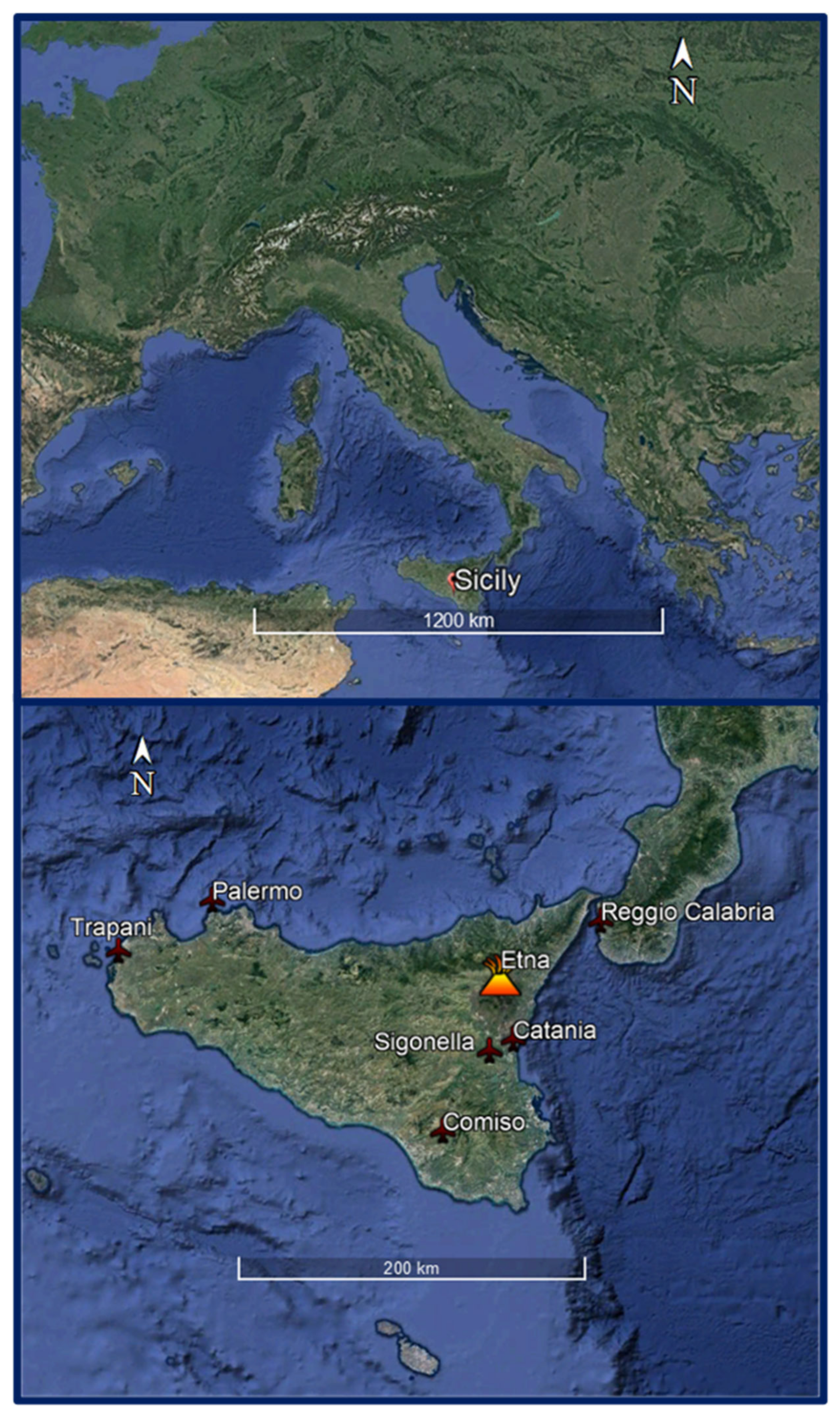
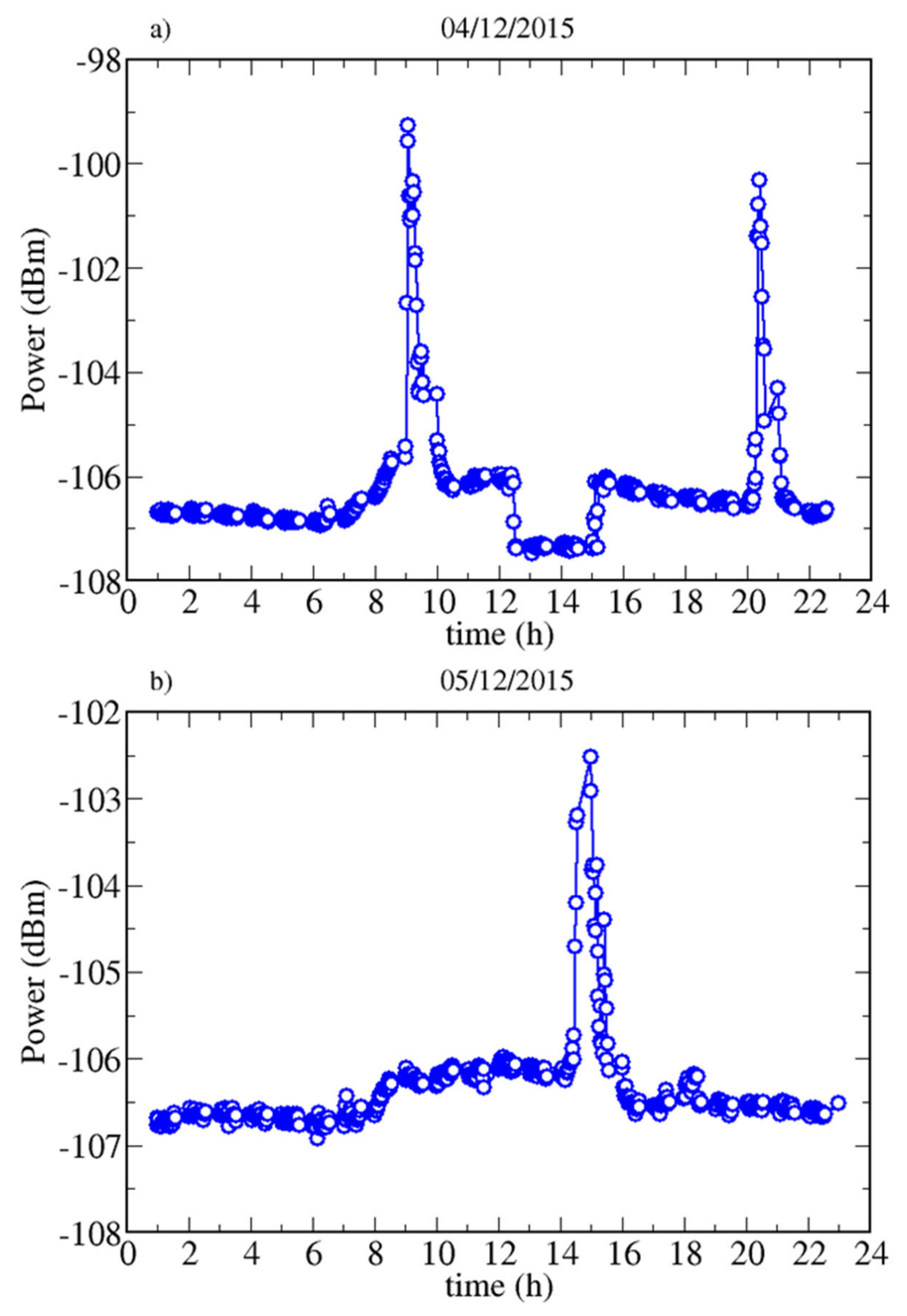
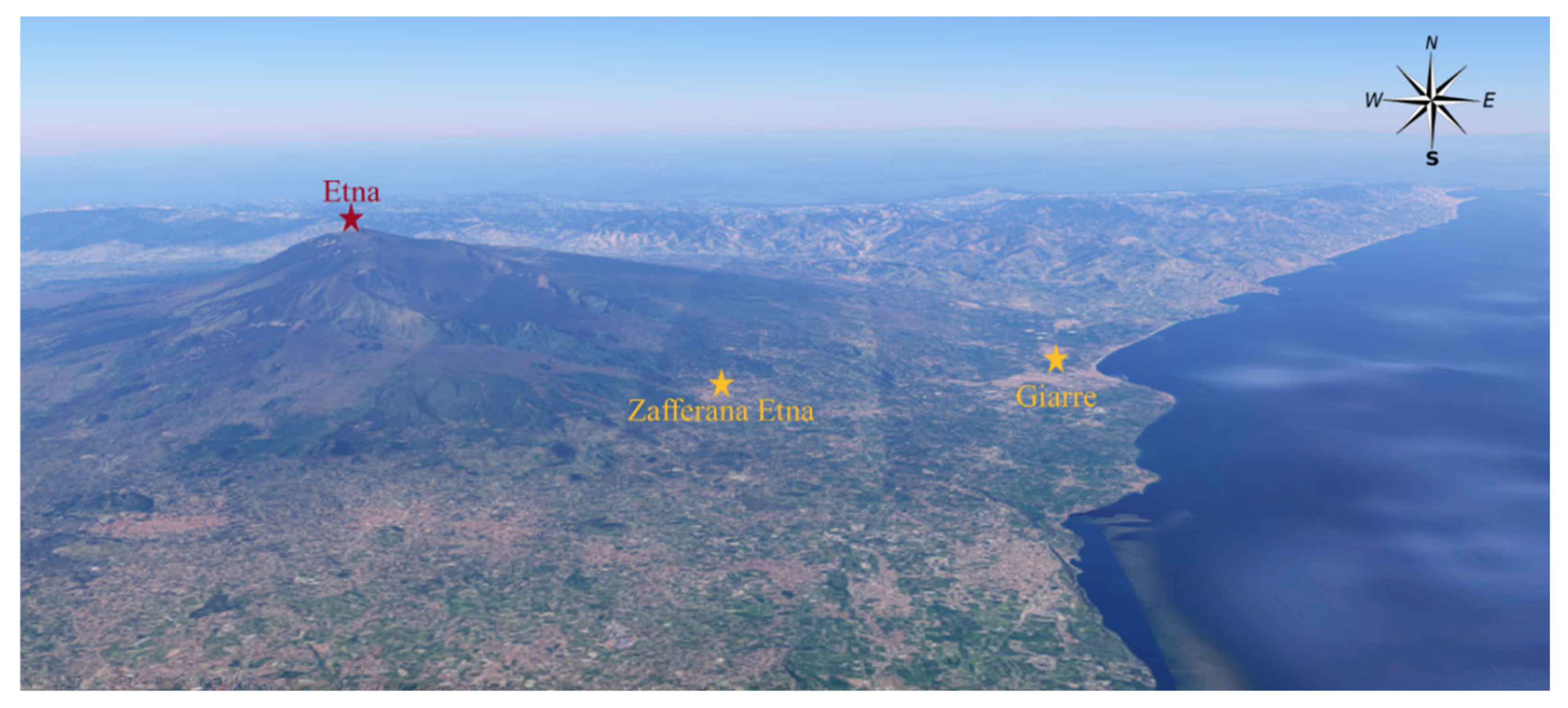
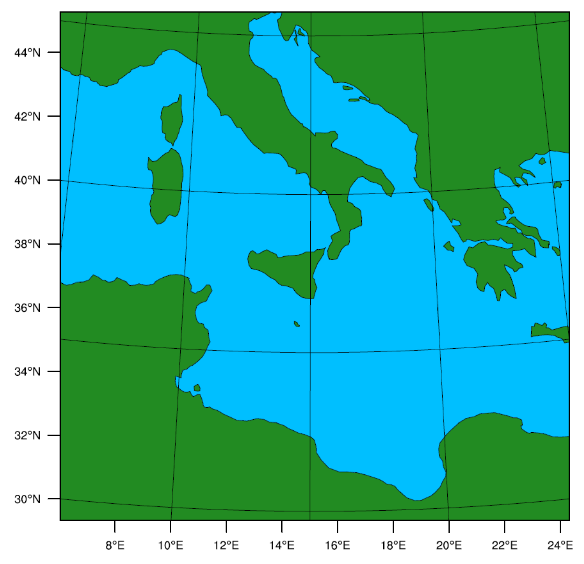
2. Case Study: December 2015

From December 3rd–7th, 2015, at Etna volcano, an explosive event occurred; it lasted about a week and was characterized by various episodes of different intensity. Moreover, these events had repercussions on the air traffic; in fact, the Catania International Airport reported numerous closures due to the volcanic ashes accumulated on the runway. In the weeks before the explosive event, constant strombolian activity (explosions of varying intensity and frequency, with the casting of incandescent material sometimes accompanied by small amounts of volcanic ash) was observed inside the Voragine crater (often called “central”), one of the four summit craters of Etna. The strombolian activity intensified on the evening of December 2th, culminating in a brief, but very violent, paroxysm on the night of December 3th. Around 02:20 UTC, the monitoring tools recorded the beginning of the eruption, which remained active until around 03:10 UTC. The eruption column exceeded 3 km in height above the vent, accompanied by volcanic explosions and lightning inside the ash cloud formed above the Voragine crater. The recorded data, obtained through the Voldorad Doppler radar, detected a signal/noise ratio of +18 dB and a longitudinal speed at the beam axis equal on average to 50 m s−1, with peaks of 60 m s−1. The eruption of December 3th was followed by three other similar paroxysmal episodes: two occurred on December 4th, respectively between 09:00 and 10:15 UTC and between 20:27 and 21:17 UTC, while the other one was detected in the afternoon of December 5th between 14:40 and 16.20 UTC. Figure 2 shows the intensity measurements of the volcanic activity (power), expressed in decibel-milliwatt (dBm) and taken from the database of the Physique du Globe de Clermont-Ferrand University [41]. Such data, captured by the OPGC Doppler radar (VOLDORAD 2B), provides immediate information on the eruption intensity by means of near-source measurements of echo power.
These three events were the most significant of the whole series of eruptions that affected Etna in this period of intense explosive activity. The eruption that occurred on the morning of December 4th was characterized by eruptive columns that reached about 7 km in height above the top of the volcano in about 15 min and at the same time frequent emissions of brown-greyish ash from a new crater were observed, along with high amplitude of volcanic tremor and strombolian explosions. The coarser pyroclastic material was deposited on the high south-western side of the volcano, at an elevation of about 2 km, while the ash fallout occurred in its eastern sector, covering the Giarre-Zafferana Etnea area. A representative map showing the position of Giarre and Zafferana Etnea with respect to Etna volcano is given in Figure 3.
The paroxysms that occurred on the evening of December 4th and in the afternoon of December 5th had almost the same characteristics as the previous ones, but the radial speed of the particles ejected by the volcano and the intensity of the volcanic activity (still measured by means of echo power) substantially decreased. In the late evening of December 5th, only degassing phenomena have been observed. At the dawn of the following day, the strombolian activity moved to the New Southeast Crater (NSEC), followed by landslides of unstable material (mixed with fragments of hot lava), which in a short time turned into pyroclastic flows. At the same time, a seismic swarm occurred in the north-eastern slope of Etna, probably connected with the volcano deflation due to the removal of a significant amount of magma: this deflation can be connected to the response of the tectonic structures in the eastern flank of the volcano. After about a week, the situation became normal again, and the explosive event finished.

3. The WRF–Chem Model

The numerical simulation of the eruptive event was carried out by means of the WRF–Chem model [18] in version 3.6.1 [42]. It consists of a type of “online” model, as it allows the evaluation of the meteorological fields together with the emission, transport, dispersion, and sedimentation of all anthropogenic and natural pollutants. In such a framework, it is possible to consider both physical processes and chemical transformations of aerosol particles released during volcanic eruptions. This key characteristic has been shown to significantly improve the accuracy of model forecasts in comparison with offline models [43]. Indeed, it is worth noting that, although weather conditions are the main factor that determines air quality, they may also depend on the direct and indirect effects that aerosol compounds have on the solar radiation and on the cloud microphysics. Most of the Volcanic Ash Transport and Dispersion (VATD) approaches are “offline” models, since they separately describe the physics and chemistry characterizing the dispersion of volcanic emissions into the atmosphere, and generally, given their low computational cost, they are largely adopted by the operational forecasting centers. However, it is more realistic to privilege the “online” approach, since an inappropriate treatment of atmospheric processes and their feedback with aerosol components could lead to incorrect predictions concerning the deposition of the ash and the diffusion of aerosols [43,44].
The WRF–Chem is based on the WRF model [17,45,46,47,48], which supports both research applications and operational meteorological forecasting applications [49], including various options for dynamic cores and physical parameterizations [50]: therefore, it can be used to simulate atmospheric conditions on a wide range of space and time scales. The chemical package that simulates tracer gases and aerosol interactively with the meteorological fields making use of different photochemical treatments and aerosols models has been integrated by using the WRF–ARW numerical core [51]. Among others, the WRF–Chem model can be used to forecast and simulate meteorological/climatic conditions on a regional and local scale, predicting the release and transport of pollutants and natural aerosols [52], estimating the air quality, and studying important processes for global climate change [35]. The capability of the model to predict the transport and concentration of ash clouds and SO2 depends on the initial information regarding volcanic emissions, such as the scale of the eruption (which includes the expelled mass), the height of the plume above the vent, the eruption rate, the date, and duration of the event [27,53].
In our simulations, the spectrum of the grain size distribution of the ash particles has been taken from Stuefer et al. [27]. In particular in their Table 1, adapted from M09 [6], they classified Eruption Source Parameters (ESP) for Etna as “small mafic”, or M1 [24].
Figure 4 shows the numerical domain adopted in the present work: this domain includes a part of North Africa, Italy, and a part of Balkan Europe, with a 180 × 180 grid centered at a latitude of 37.74° and longitude of 15.18°. The horizontal space of the grid is 10 km in both directions with 40 vertical levels up to 50 hPa. The initial and boundary conditions were acquired by NCAR/NCEP Final Analysis (FNL by GPS) (ds083.2), with resolution of 1 degree, every six hours [54].
Table 1 shows the physical schemes selected for the setting of the parameterizations, specifically Mellor-Yamada-Nakanishi and Niino (MYNN, level 2.5) for the planetary boundary layer [55], surface similarity [56], and the surface model RUC (rapid update cycle) [57]. These schemes have been chosen to represent the physics of the surface layer and the parametrization of the Earth’s surface. The Rapid Radiative Transfer Model (RRTMG) for both short-wave (ra_sw_physics = 4) and long-wave (ra_lw_physics = 4) radiation is used for the direct radiative effect of aerosol [58]. The Purdue Lin scheme (mp_physics = 2) is used for microphysics processes. This configuration is compatible with short-wave radiative feedback [59].
The implementations of the other parameters follow the guidelines of Stuefer et al., 2009 [27] (such as the mass of volcanic ash, set to 1.7 × 10⁹ kg), or are based on estimates derived from the literature (as for the mass of SO2 set to 1.0 × 10⁹ kg) [60]. These parameters are reported in Table 2: for the injection heights above the vent and duration, the observations taken from the cameras and radar Doppler VOLDORAD 2B [39] have been adopted. Such a radar is placed at approximately 3 km from the top of the volcano and has been made available by the Observatoire de Physique do Globe de Clermont-Ferrand (OPGC) in collaboration with the Istituto Nazionale di Geofisica e Vulcanologia (INGV) of Catania.

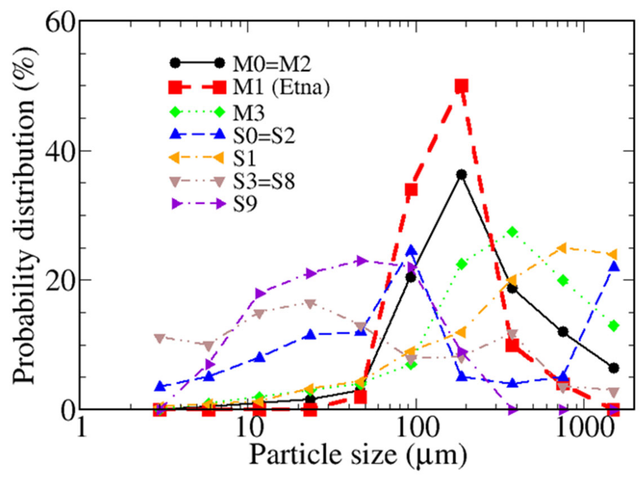
4. Semi-Empirical Description of Eruption Processes and Input Parameters of the WRF–Chem Model

The classification drawn up by M09 is based on the study of well-documented past eruptions and includes eleven types of eruptions. If new observations reveal data different from the predefined ones, one needs to find the type of eruption closest to the one under study and use its parameters. Stuefer et al., 2013 [27], divided the granulometric size spectrum of the ash particles into 10 bins (in their Table 2) and coded them within the WRF–Chem software. This classification considers particles’ diameter in a range going from 2 mm to less than 3.9 μm and the corresponding percentage of the mass fraction depending on the type of Eruption Source Parameters (ESP). The latter are needed to predict the transport and dispersion of volcanic ash clouds during eruptions, with the aim of identifying risks for the air navigation. For each ash-bin (Table 3), it is possible to define the aerodynamic radius as half of the arithmetic mean between the limits of the diameters of each ash-bin. The erupted mass is distributed in the so-called umbrella cloud model, for which it is assumed that 75% of the erupted mass is detrained in the umbrella cloud and 25% beneath, with a linear distribution from the umbrella to the vent [27].
According to M09, all the possible eruption categories may be classified as M-type, or mafic types, which include basaltic and ultramafic magmas; and S-type, or silicic types, which include andesite, dacite, rhyolite, and others such as phonolite that can produce high ash columns (M09, Table 3, pag.16). As far as Etna is concerned, the M09 classification assigned the class M1 to its eruptions, which are mainly of an effusive type, i.e., they are characterized by basaltic dense-lava fountains, with relatively high temperatures (>1000 °C). In Table 3, it is reported the particle size distribution assigned to the emitted particles diameters in the range between 1000 μm and 31.25 μm.
It has been formulated considering for Etna a grain distribution that has been obtained by the semi-empirical methodology defined by Scollo et al. [24]. According to the classification reported in the table, 4% of particles have a diameter between 0.5 and 1 mm (vash_2), 10% between 0.25 and 0.5 mm (vash_3), 50% between 125 and 250 μm (vash_4), 34% between 62.50 and 125 μm (vash_5), and 2% between 31.25 and 62.50 μm (vash_6). No particles with diameter less than 31.25 μm are considered [27]. It is evident from Table 3 that smaller particles (bins 7–10) are not considered in M1 classification. In this context, it may be crucial for future studies to consider in-situ measurements, for example from an Optical Particle Counter, for the direct measurement of the size distribution of volcanic aerosols after the Etna eruption [61].
In Figure 5, the distributions of volcanic ash emitted by Etna (M1) are compared with those observed in different classes of eruptions, according to the database by M09. In this figure, each point represents the midpoint of each bin reported in Table 3, as stated above. It emerges that the distribution of Etna ash shows a well-defined peak at a particle size of 175 μm, with about 50% of emitted particles having this size. In addition, it is worth noting that this is the less polydisperse distribution, with only five values other than zero. These findings suggest that this particular class of eruptions may attain very high temperatures in order to generate a huge amount of particles of relatively large size with a low degree of polydispersity and this result should likely be verified by local measurements as stated above. It is worth noting that also different total grain size distributions could be adopted for the Etna volcano, such those reported in Ref. [62]. In future studies, we plan to compare these different distributions in order to assess how the ash dispersion and transportation depends on their spectrum in the WRF–Chem model.
The input parameters of the WRF–Chem model are determined by using a software pre-processor called PREP–CHEM–SRC [63], developed to prepare the grid emission parameters for the most important anthropogenic pollutants. In this work, the Version 1.5 of the PREP–CHEM–SRC has been employed. Such a pre-processor is specifically designed to include input parameters concerning volcanic eruptions. Once the height of the plume above the vent and the eruption duration are defined, the total erupted mass can be estimated according to the following equation, holding for volcanic ash only (see M09):
M = ρd(0.5 h)4.1494
where M is the mass eruption rate (in kg), ρ is the ash density (in kgm−3), d the eruption duration (in s), and ρ the plume height (in km) above the vent.
Moreover, the PREP–CHEM–SRC provides the position of the volcano in the numerical domain considering the nearest grid cell.
It is important to mention that in addition to the ash, during a volcanic eruption, a considerable amount of SO2 is also emitted, which, once in the atmosphere, oxidizes and transforms into sulfuric acid (H2SO4); the latter condenses into sulfate aerosols, characterized by a residence time in the atmosphere proportional to the gases containing sulfur present in the volcanic plume. Unlike the ash that settles within few days, SO2 can last up to several months [12].
The data provided by the international program AEROCOM (started in 2002 with the target to reduce the uncertainty on the impact of aerosols on the climate system) contain the volcanic emissions of SO2 and other variables for the time interval going from January 1979 to December 2009 for all the volcanoes listed in the Global Volcanism Program database provided by the Smithsonian Institution. In particular, there is a file for each year containing the number of events occurred, along with the name of the volcano, the date, the height above the average sea level, the height of the plume above the vent, the longitude, the latitude, and the daily emission rate of SO2, distinguishing between volcanic eruptive and non-eruptive emissions. In analogy with the preprocessing phase of ash emissions, the SO2 emissions are placed in a grid point of the spatial domain, which includes the position of the investigated volcano. The total SO2 emission corresponds to the amount of SO2 emitted by the volcano inside the grid point, and it is expressed in kg m−2 dy−1 [27].
The pre-processing tool, as in the case of volcanic ash, places the SO2 emissions in the grid point of the WRF–Chem domain that surrounds the geographical position of the investigated volcano. The total emission is calculated by adding the emissions of all the volcanoes inside the cell and is expressed in Kg km−2 hr−1. However, it is important to point out that this value is often only approximated, in consideration of the difficulty usually met in accurately estimating the correct total amount of SO2 emitted during a volcanic eruption.

5. Results and Discussion
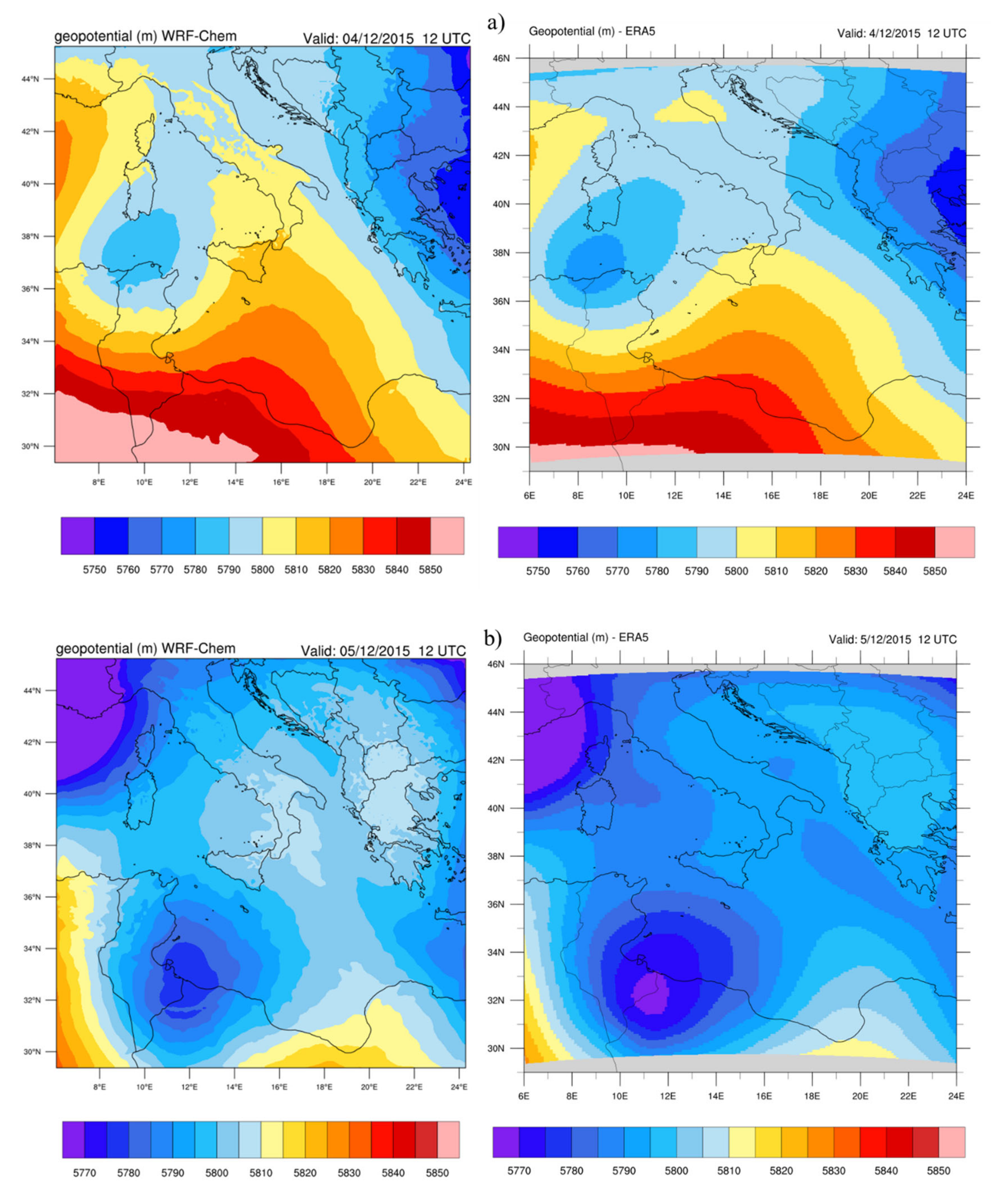
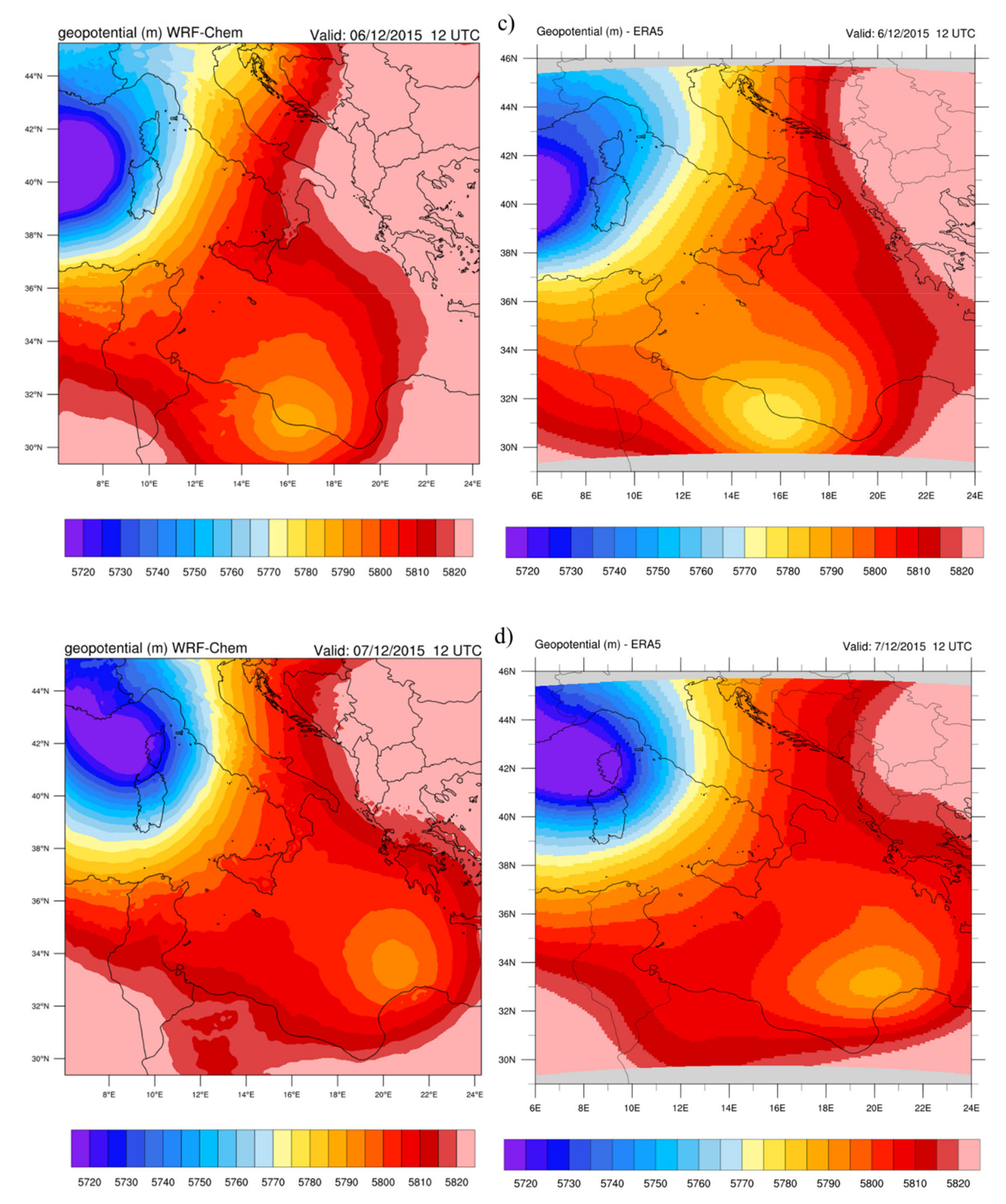
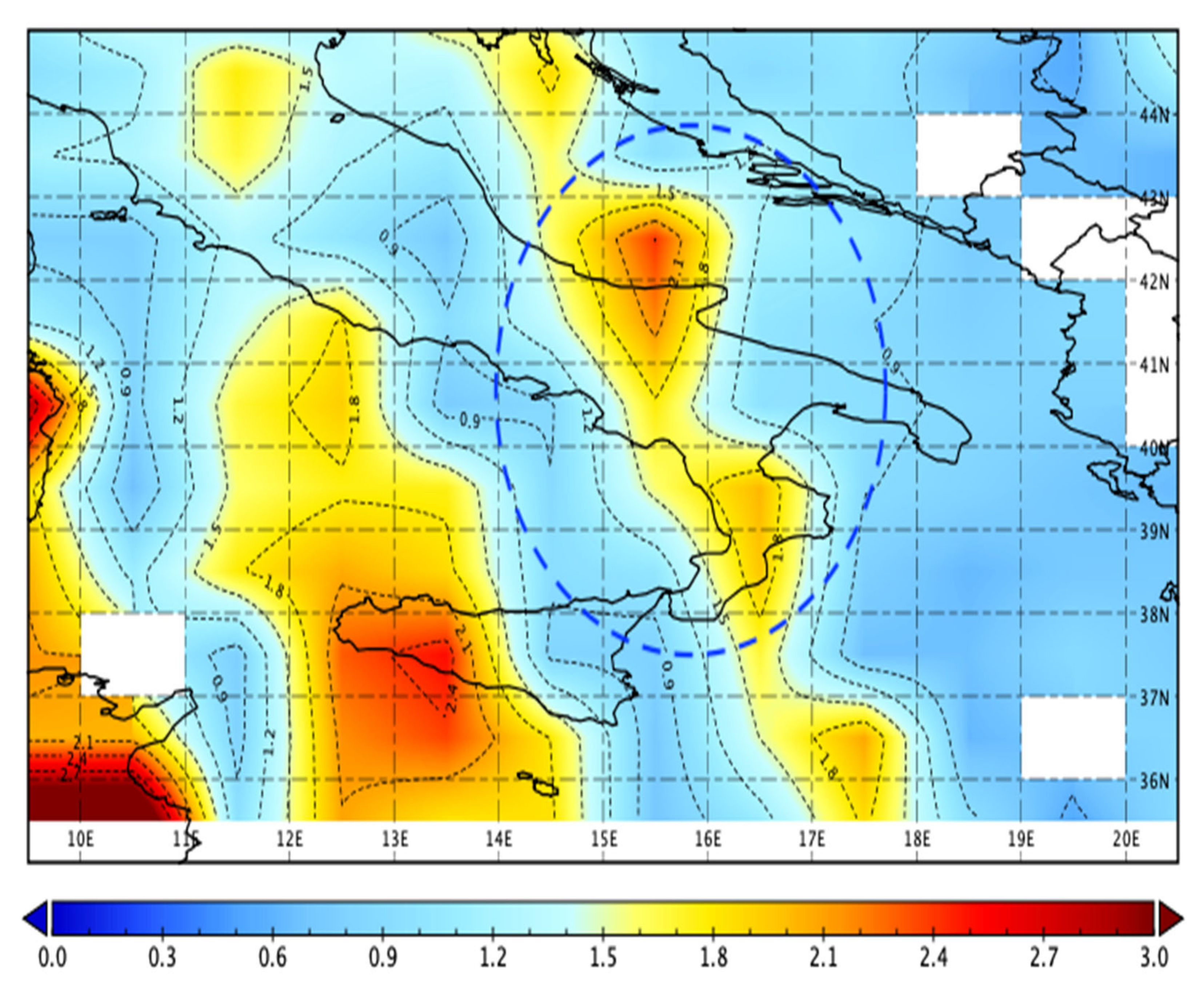
5.1. Geopotential

In Figure 6a–d, the comparison between the geopotential height at an atmospheric pressure of 500 hPa predicted by the WRF–Chem (left panels) and data downloaded from ECMWF/ERA5-reanalysis (right panels) is reported. ERA5-reanalysis are available from the Copernicus Climate Change Service (C3S, 2017) at the following URL (https://www.ecmwf.int/en/forecasts/datasets/reanalysis-datasets/era5) [64].
During December 4th (Figure 6a), ERA5-reanalysis (right panel) shows a pressure minimum localized between the southern coast of Sardinia and northern coast of Tunisia that fosters a south-east circulation near Etna. The following day, December 5th (Figure 6b, right panel), ERA5-reanalysis depicts that the pressure minimum is further dislocated toward the south entering the African continent near the Tunisia/Libyan border. The consequent circulation at Etna is rotated in the north-west direction. On December 6th, again considering ERA5-reanalysis (Figure 6c, right panel), a deepening of the low pressure between Balearic Islands and Sardinia producing northward wind near Etna is evident. Finally, on December 7th, when the eruptive intensity started to decrease, ERA5-reanalysis (Figure 6d, right panel) shows that the cyclonic system moved in the north-west direction toward the southern coast of France, inducing a northern flow near Etna. The close agreement between the ERA5 (Figure 6, right panels) geopotential at 500 hPa and the WRF–Chem model is evident (Figure 6, left panels). This is quite important, as the dispersion of eruptive plumes of ashes and gases (SO2) is strictly connected with wind speed and direction.

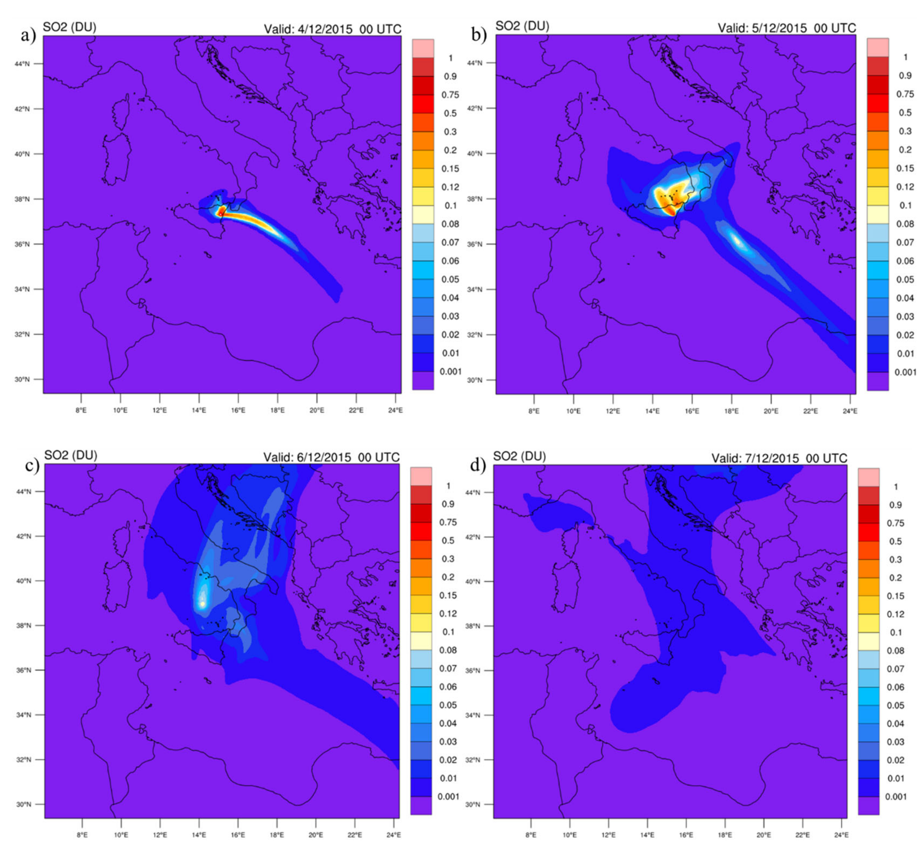
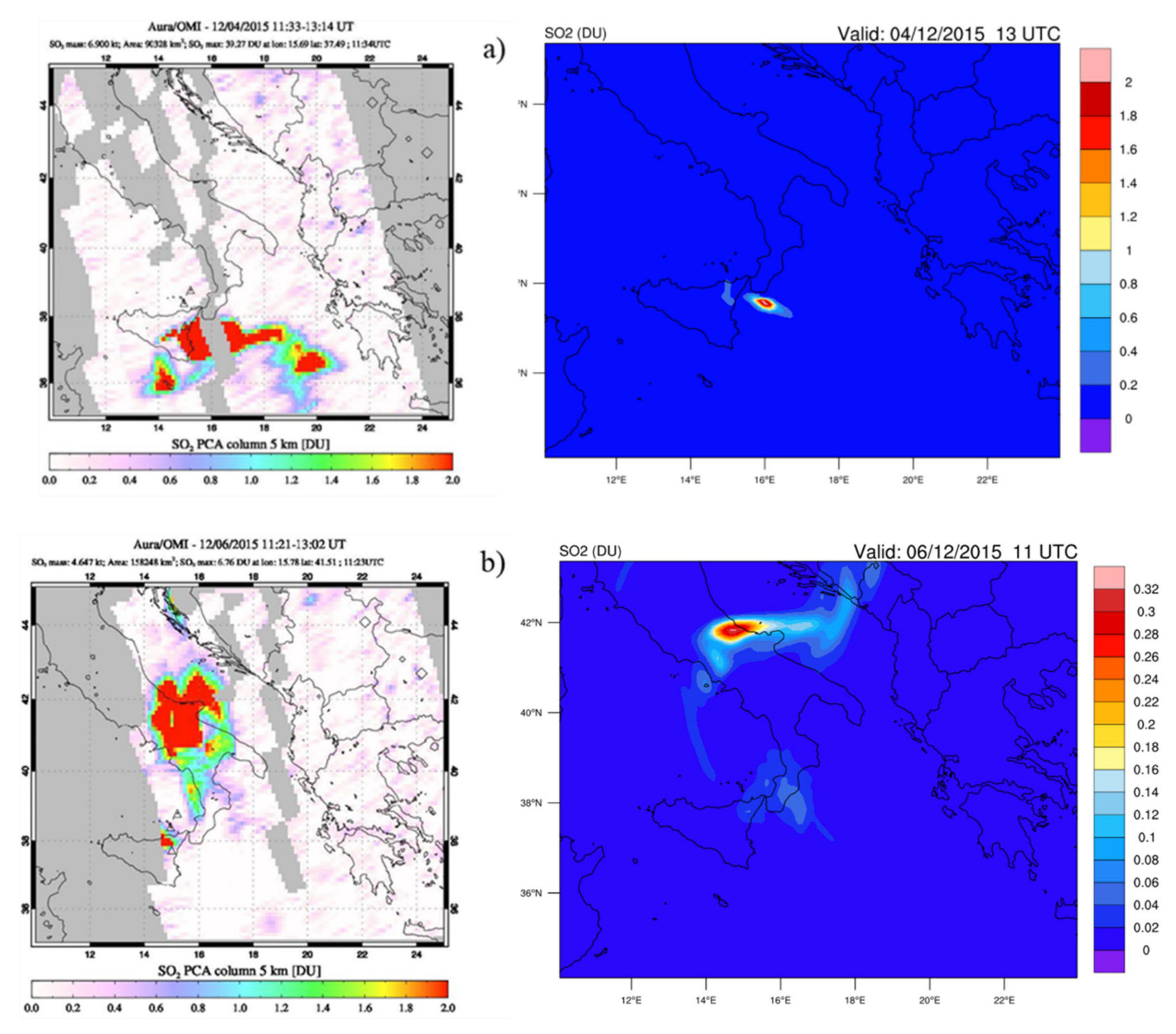
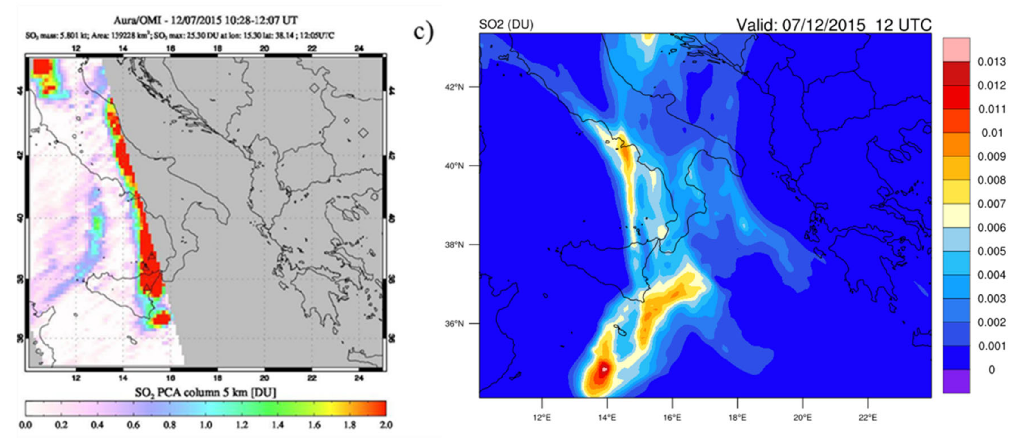
5.2. Transport of SO2

Sulfur dioxide (SO2) is a colorless, irritating, non-flammable gas, very soluble in water and with a pungent smell. This compound is one of the most widespread, dangerous, and studied atmospheric pollutants. It derives from the oxidation of sulfur during the combustion processes of substances that contain this element. Due to the characteristics of sulfur dioxide, it is interesting to analyze its distribution in the course of the studied event. At this purpose, the daily data relating to the columnar density of SO2, expressed in Dobson Units (DU), have been downloaded from the NASA/Earthdata program [66] through one of its dedicated web-portals [67]. The DU indicates the concentration of gas in a column of air, above a certain point on the Earth’s surface. The daily SO2 total column data have been provided by the EOS-Aura satellite [68] via the OMI sensor (Ozone Monitoring Instrument) with a spatial resolution of 0.25° × 0.25°. The SO2 observational data have been compared with the output of the WRF–Chem model: the latter have been first averaged over a single day and then column-integrated in every surface grid point, finally providing values expressed in DU. The conversion factor is: 1 DU 28,000 μg m−2.
The WRF–Chem simulations allow the analysis of the spatial distribution of daily averaged sulfur dioxide emitted during the eruptive event under investigation. The scale of the daily average SO2 concentrations shown in Figure 7 identifies values ranging from 0 to 1 DU. In particular, on December 4th (Figure 7a), there is an intense emission of SO2 that spreads out mainly to the south-east with a plume that crosses the Mediterranean until it almost reaches the coast of Africa.
Between December 5th and 7th (Figure 7b–d) another intense flow of SO2 from Etna is transported to the north, covering the entire Italian southern peninsula. In this context, it may be evidenced that the results of the simulations provide a spatial distribution of the daily average SO2 that reflects in a fairly precise way the synoptic analysis and the description of the event discussed above (see Figure 6).
A comparison between the results obtained by using the WRF–Chem model and the daily data retrieved by the Aura satellite via the OMI sensor has been also performed. At 13:00 UTC on December 4th, immediately after the paroxysm, the OMI map reports approximately the same distribution of SO2, characterized by a shift of the flow towards the south-east (Figure 8a). According to the simulation results, the SO2 concentration amounts to approximately 1.8 DU, close enough to the observed value of about 2 DU. Due to the lack of satellite data, it is not possible to make a comparison on December 5th. On December 6th (Figure 8b), there is a good qualitative correspondence between the spatial distribution predicted by the model and that provided by the satellite, albeit the amount of SO2 appears slightly underestimated by the simulations. In particular, it is possible to observe from both maps the transport of the SO2 to the north, up to the Gargano and the Adriatic regions. Finally, with reference to December 7th (Figure 8c), both maps show that sulfur dioxide, spread to central Italy, decreased in concentration, although it is not possible to explain the presence of an abundant quantity of SO2 recorded by the OMI sensor between Sicily and Calabria. The origin of this discrepancy can be ascribed to the fact that in the WRF–Chem approach, we simulate only the three main events (see Table 2), whereas puffs of erupted material can be expected along the entire duration of the event (degassing). Despite the discrepancy observed on the last day of the eruption, the overall distribution of SO2 along the whole duration of the process appears fairly well reproduced by the WRF–Chem model.

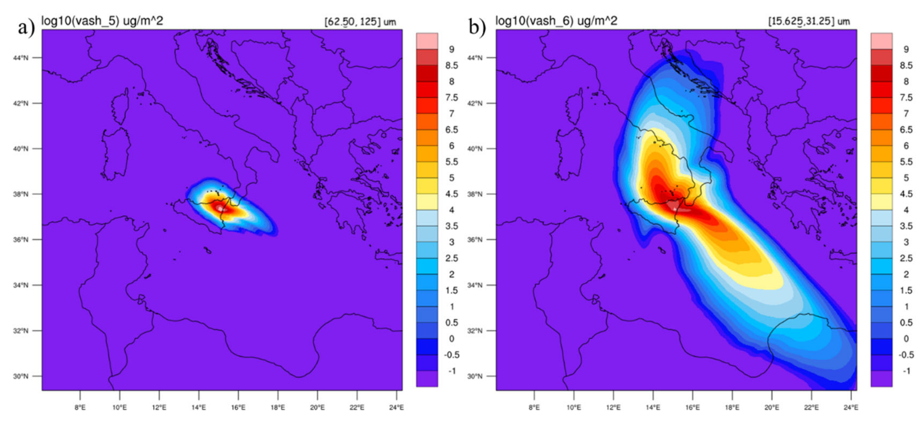
5.3. Distribution of Volcanic Ash

In addition to the SO2, in this study the transport of ash particles of different sizes has been analysed for the time interval from December 4th to 7th.
It is important to mention that in its default configurations, the WRF–Chem model uses the Stokes law corrected by the Cunningham slip factor [27] for calculating the terminal fall velocity. This is well suited for small particles only (typically with a diameter < 0.125 mm). Such an issue could be solved by implementing in the WRF–Chem model different formulations of the settling velocity, as detailed, for instance, in Refs. [69,70,71,72]. In this context, for the following analysis, we showed results only for vash_5 and vash_6 particles. As reported in Figure 9, the average values of the different vash sizes range between 10−1 and 108 μg m−2. These data, expressed as mass per unit area, have been obtained by integrating the column load. It is observed that the larger particles (vash_5), being heavier, have fallen back into the areas adjacent to the volcano, while the finer ones (vash_6), and therefore lighter, have been transported to greater distances, reaching central Italy and the African coast.
In order to validate the model predictions, the simulation results have been compared with observed data characterized by the Aerosol Index (AI), explicitly developed to detect the presence of aerosols in the air. The aerosol measurements were carried out again by the OMI sensor on board the above-described NASA/Aura spacecraft. In Figure 10, the area circumscribed by the dashed line highlights the regions affected by the dispersion of aerosols due to the eruption of Etna, showing how the suspension of particles is spread mainly over Sicily, the Mediterranean Sea, and the Gargano, in agreement with the wind circulation derived from the synoptic analysis previously described. There are also high concentrations of aerosols (orange coloring) in the south-east part of Sicily, but since the wind mainly blew northwards during the paroxysmal episodes, this can be ascribed to dust from the Sahara. A qualitative agreement with the WRF–Chem results is clearly visible, albeit a more detailed comparison is not possible due to the different units adopted.
A further analysis has been done considering only the volcanic ash with diameter between 15.62 and 31.25 μm (vash_7) that, according to M09 distribution reported in Table 3, should not be present for M1 class. Therefore, the starting amount of vash_7 has been set by choosing that corresponding to the M2 classification (see M09); according to this prescription, the percentage of vash_7 particles is 1.5% of the total ash. This supplementary study aims to investigate the transport of small particles in the numerical domain. In Figure 11a, the WRF–Chem predictions on the transport of vash_7 are shown: as observed, in this case, the finest volcanic particles can be found in the eastern regions of Europe. Finally, in Figure 11b, the amount of vash_7 that exceeds the detection limit of satellite-based ash retrieval algorithms of 0.1 g m−2 is reported. Even if we only consider vash_7, the large distribution of volcanic ash above the threshold limit that may be considered potentially dangerous for any flight operations is evident. This aspect needs to be further investigated and verified by future studies by considering the LIDAR measurements network in Europe [73,74] or the satellite retrievals from the Spinning Enhanced Visible and Infrared Imager (SEVIRI) onboard the Meteosat Second Generation spacecraft.

6. Conclusions

In this work, we have presented an application of the WRF–Chem model to systematically investigate the Etna volcanic eruption registered at the beginning of December 2015 and its role in affecting the security of the airports involved as well as the transportation of pollutants and volcanic ash in the Mediterranean area. As far as the case study considered is concerned, the WRF–Chem model has proved to be an excellent candidate for the prediction of the transport and dispersion of natural and anthropogenic aerosols, as well as for volcanic ash and sulfur dioxide emitted during the volcanic eruption. In this study, the output obtained from the numerical model agrees with the satellite retrievals and with the meteorological reanalysis. It has been possible to reconstruct the dynamics of Etna volcanic ash transport and to confirm the data concerning both the concentration and the direction of propagation of ash and gases emitted into the atmosphere.
More in detail, immediately after the first paroxysm, the ejected material was transported towards the north-east by winds. Then, the circulation underwent a south-east rotation and, at the end of the eruptive event, the volcanic cloud overlooked the skies of southern Italy, up to the Gargano, the Balkans, and the African coast. Concentrations of SO2, of the order of 1.8 DU, were recorded in the time bands of maximum explosive activity, which progressively decreased to a few tenths. The particles expelled during the eruption reached maximum concentrations 2.0 DU, and the finest ones (vash_6) went as far as the Balkans and Africa, while those with a larger diameter (vash_5) fell back in the areas surrounding Etna mountain.
Although the model has exhaustively reproduced the event, it is advisable to modify the WRF–Chem input settings, especially with regard to the particle size distribution to be adopted. The results, obtained by simulating the transport of volcanic ash including particles having dimensions between 15.62 and 31.25 μm (vash_7), suggest the possible spreading out of Etna volcanic ash until the east of Europe. Upon summarizing the model predictions and the relative comparison with the observed data, it emerges that the WRF–Chem model can be a valid support both to airport management companies affected by volcanic emission phenomena and to other local stakeholders such as public administrations. In addition, the capability of the model to describe the diffusion of Etna volcanic ash and SO2 in the atmosphere is particularly useful in order to better understand the impact of this volcano on the meteorological phenomena involving the whole Mediterranean area. Additional developments of the WRF–Chem model aiming to further increase the accuracy of the predictions are currently underway, as well as the comparison with different models, including FALL3D [32], HYSPLIT [75], and Ash3d [76].

Author Contributions

All authors contributed to conceptualization, methodology, investigation, writing, reviewing, and editing of the present work. All authors have read and agreed to the published version of the manuscript.

Funding

This work is to be framed within the Progetto di Ricerca e Sviluppo “Impiego di tecnologie, materiali e modelli innovativi in ambito aeronautico (AEROMAT)”, Asse II “Sostegno all’innovazione”, Area di Specializzazione “Aerospazio” Avviso n. 1735/Ric del 13 luglio 2017 - Codice CUP J66C18000490005, codice identificativo Progetto ARS01_01147 nell’ambito del Programma Operativo Nazionale “Ricerca e Innovazione” 2014–2020 (PON R&I 2014–2020).

Acknowledgments

Analyses and visualizations used in this paper were produced with the Giovanni online data system, developed and maintained by the NASA GES DISC.

Conflicts of Interest

The authors declare no conflict of interest.

References

  1. Wilson, G.; Wilson, T.M.; Deligne, N.I.; Cole, J.W. Volcanic hazard impacts to critical infrastructure: A review. J. Volcanol. Geoterm. Res. 2014, 286, 148–182. [Google Scholar] [CrossRef] [Green Version]
  2. Curtius, J. Nucleation of atmospheric aerosol particles. Comptes Rendus Phys. 2006, 7, 1027–1045. [Google Scholar] [CrossRef]
  3. Castorina, G.; Caccamo, M.T.; Magazù, S.; Restuccia, L. Multiscale mathematical and physical model for the study of nucleation processes in meteorology. AAPP 2018, 96. [Google Scholar] [CrossRef]
  4. Hanstrum, B.N.; Watson, A.S. A case study of two eruptions of Mount Galunggung and an investigation of volcanic eruption cloud characteristics using remote sensing techniques. Aust. Met. Mag. 1983, 31, 131–177. [Google Scholar]
  5. Davies, C.N. Size distribution of atmospheric particles. J. Aerosol. Sci. 1974, 5, 293–300. [Google Scholar] [CrossRef]
  6. Mastin, L.G.; Guffanti, M.; Servranckx, R.; Webley, P.; Barsotti, S.; Dean, K.; Durant, A.; Ewert, J.W.; Neri, A.; Rose, W.I.; et al. A multidisciplinary effort to assign realistic source parameters to models of volcanic ash-cloud transport and dispersion during eruptions. J. Volcanol. Geotherm. Res. 2009, 186, 10–21. [Google Scholar] [CrossRef]
  7. Diehl, T.; Heil, A.; Chin, M.; Pan, X.; Streets, D.; Schultz, M.; Kinne, S. Anthropogenic, biomass burning, and volcanic emissions of black carbon, organic carbon, and SO2 from 1980 to 2010 for hindcast model experiments. Atmos. Chem. Phys. Discuss. 2012, 12, 24895–24954. [Google Scholar] [CrossRef] [Green Version]
  8. Schoeber, M.R.; Doiron, S.D.; Lait, L.R.; Newman, P.A.; Krueger, A.J. A simulation of the Cerro Hudson SO2 cloud. J. Geophys. Res. Atmos. 1993, 98, 2949–2955. [Google Scholar] [CrossRef]
  9. Carn, S.A.; Yang, K.; Prata, A.J.; Krotkov, N.A. Extending the long-term record of volcanic SO2 emissions with the Ozone Mapping and Profiler Suite nadir mapper. Geophys. Res. Lett. 2015, 42, 925–932. [Google Scholar] [CrossRef] [Green Version]
  10. Li, C.; Krotkov, N.A.; Carn, S.; Zhang, Y.; Spurr, R.J.D.; Joiner, J. New-generation NASA Aura Ozone Monitoring Instrument (OMI) volcanic SO2 dataset: Algorithm description, initial results, and continuation with the Suomi-NPP Ozone Mapping and Profiler Suite (OMPS). Atmos. Meas. Tech. 2017, 10, 445–458. [Google Scholar] [CrossRef] [Green Version]
  11. Prata, A.J.; Bernardo, C. Retrieval of volcanic SO2 column abundance from Atmospheric Infrared Sounder data. J. Geophys. Res. Atmos. 2007, 112, D20204. [Google Scholar] [CrossRef]
  12. McCormick, M.P.; Thomason, L.W.; Trepte, C.R. Atmospheric effects of the Mt Pinatubo eruption. Nature 1995, 373, 399–404. [Google Scholar] [CrossRef]
  13. Robock, A. Volcanic eruptions and climate. Rev. Geophys. 2000, 38, 191–219. [Google Scholar] [CrossRef]
  14. Frolicher, T.L.; Joos, F.; Raible, C.C. Sensitivity of atmospheric CO2 and climate to explosive volcanic eruptions. Biogeosciences 2011, 8, 2317–2339. [Google Scholar] [CrossRef] [Green Version]
  15. Wang, X.; Boselli, A.; D’Avino, L.; Pisani, G.; Spinelli, N.; Amodeo, A.; Chaikovsky, A.; Wiegner, M.; Nickovic, S.; Papayannis, A.; et al. Volcanic dust characterization by EARLINET during Etna’s eruptions in 2001–2002. Atmos. Environ. 2008, 42, 893–905. [Google Scholar] [CrossRef]
  16. Tanguy, J.C.; Condomines, M.; Le Goff, M.; Chillemi, V.; La Delfa, S.; Patanè, G. Mount Etna eruptions of the last 2,750 years: Revised chronology and location through archeomagnetic and 226Ra-230Th dating. Bull. Volcanol. 2007, 70, 55–83. [Google Scholar] [CrossRef]
  17. Skamarock, W.C.; Klemp, J.B. A time-split nonhydrostatic atmospheric model for weather research and forecasting applications. J. Comput. Phys. 2008, 227, 3465–3485. [Google Scholar] [CrossRef]
  18. Grell, G.A.; Peckahm, S.E.; Schmitz, R.; McKeen, S.A.; Frost, G.; Skamarock, W.C.; Eder, B. Fully coupled “online” chemistry within the WRF model. Atmos. Environ. 2005, 39, 6957–6975. [Google Scholar] [CrossRef]
  19. Misenis, C.; Zhang, Y. An examination of sensitivity of WRF/Chem predictions to physical parameterizations, horizontal grid spacing, and nesting options. Atmos. Res. 2010, 97, 315–334. [Google Scholar] [CrossRef]
  20. Donnadieu, F.; Freville, P.; Hervier, C.; Coltelli, M.; Scollo, S.; Prestifilippo, M.; Valade, S.; Rivet, S.; Cacault, P. Near-source Doppler radar monitoring of tephra plumes at Etna. J. Volcanol. Geotherm. Res. 2016, 312, 26–39. [Google Scholar] [CrossRef]
  21. Freret-Lorgeril, V.; Donnadieu, F.; Scollo, S.; Provost, A.; Fréville, P.; Guéhenneux, Y.; Hervier, C.; Prestifilippo, M.; Coltelli, M. Mass Eruption Rates of Tephra Plumes During the 2011–2015 Lava Fountain Paroxysms at Mt. Etna From Doppler Radar Retrievals. Front. Earth Sci. 2018, 6, 73. [Google Scholar] [CrossRef]
  22. Favalli, M.; Karatson, D.; Mazzarini, F.; Pareschi, M.T.; Boschi, E. Morphometry of scoria cones located on a volcano flank: A case study from Mt. Etna (Italy), based on high-resolution LiDAR data. J. Volcanol. Geotherm. Res. 2009, 186, 320–330. [Google Scholar] [CrossRef]
  23. Andronico, D.; Spinetti, C.; Cristaldi, A.; Buongiorno, M.F. Observations of Mt. Etna volcanic ash plumes in 2006: An integrated approach from ground-based and polar satellite NOAA–AVHRR monitoring system. J. Volcanol. Geotherm. Res. 2009, 180, 135–147. [Google Scholar] [CrossRef]
  24. Scollo, S.; Del Carlo, P.; Coltelli, M. Tephra fallout of 2001 Etna flank eruption: Analysis of the deposit and plume dispersion. J. Volcanol. Geotherm. Res. 2007, 160, 147–164. [Google Scholar] [CrossRef]
  25. Edwards, M.J.; Pioli, L.; Andronico, D.; Scollo, S.; Ferrari, F.; Cristaldi, A. Shallow factors controlling the explosivity of basaltic magmas: The 17–25 May 2016 eruption of Etna Volcano (Italy). J. Volcanol. Geotherm. Res. 2018, 357, 425–436. [Google Scholar] [CrossRef]
  26. Andronico, D.; Scollo, S.; Cristaldi, A.; Ferrari, F. Monitoring ash emission episodes at Mt. Etna: The 16 November 2006 case study. J. Volcanol. Geotherm. Res. 2009, 180, 123–134. [Google Scholar] [CrossRef]
  27. Stuefer, M.; Freitas, S.R.; Grell, G.; Webley, P.; Peckham, S.; McKeen, S.A.; Egan, S.D. Inclusion of ash and SO2 emissions from volcanic eruptions in WRF-Chem: Development and some applications. Geosci. Model. Dev. 2013, 6, 457–468. [Google Scholar] [CrossRef] [Green Version]
  28. Hirtl, M.; Stuefer, M.M.; Arnold, D.; Grell, G.; Maurer, C.; Natali, S.; Scherllin-Pisher, B.; Webley, P. The effects of simulating volcanic aerosol radiative feedbacks with WRF-Chem during the Eyjafjallajökull eruption, April and May 2010. Atmos. Environ. 2019, 198, 194–206. [Google Scholar] [CrossRef]
  29. Dacre, H.F.; Grant, A.L.M.; Hogan, R.J.; Belcher, S.E.; Thomson, D.J.; Devenish, B.J.; Marenco, F.; Hort, M.C.; Haywood, J.M.; Ansmann, A.; et al. Evaluating the structure and magnitude of the ash plume during the initial phase of the 2010 Eyjafjallajökull eruption using lidar observations and NAME simulations. J. Geophys. Res. 2011, 116. [Google Scholar] [CrossRef]
  30. Devenish, B.; Francis, P.N.; Johnson, B.T.; Sparks, R.S.J.; Thomson, D.J. Sensitivity analysis of dispersion modeling of volcanic ash from Eyjafjallajökull in May 2010. J. Geophys. Res. 2012, 117. [Google Scholar] [CrossRef]
  31. Webster, H.N.; Thomson, D.J.; Johnson, B.T.; Heard, I.P.C.; Turnbull, K.; Marenco, F.; Kristiansen, N.I.; Dorsey, J.; Minikin, A.; Weinzierl, B.; et al. Operational prediction of ash concentrations in the distal volcanic cloud from the 2010 Eyjafjallajökull eruption. J. Geophys. Res. 2012, 117. [Google Scholar] [CrossRef] [Green Version]
  32. Folch, A.; Costa, A.; Basart, S. Validation of the Fall3D ash dispersion model using observations of the 2010 Eyjafjallajokull volcanic ash clouds. Atmos. Environ. 2012, 48, 165–183. [Google Scholar] [CrossRef]
  33. Kristiansen, N.I.; Stohl, A.; Prata, A.J.; Bukowiecki, N.; Dacre, H.; Eckhardt, S.; Henne, S.; Hort, M.C.; Johnson, B.T.; Marenco, F.; et al. Performance assessment of a volcanic ash transport model mini-ensemble used for inverse modeling of the 2010 Eyjafjallajökull eruption. J. Geophys. Res. 2012, 117. [Google Scholar] [CrossRef] [Green Version]
  34. Chapman, E.G.; Gustafson, W.I.; Easter, R.C.; Barnard, J.C.; Ghan, S.J.; Pekour, M.S.; Fast, J.D. Coupling aerosol-cloud-radiative processes in the WRF-Chem model: Investigating the radiative impact of elevated point sources. Atmos. Chem. Phys. 2009, 9, 945–964. [Google Scholar] [CrossRef] [Green Version]
  35. Zhang, Y.; Wen, X.Y.; Jang, C.J. Simulating chemistry-aerosol-cloud-radiation-climate feedbacks over the continental US using the online-coupled Weather Research Forecasting Model with chemistry (WRF/Chem). Atmos. Environ. 2010, 44, 3568–3582. [Google Scholar] [CrossRef]
  36. Grell, G.A.; Freitas, S.R.; Stuefer, S.; Fast, J. Inclusion of biomass burning in WRF-Chem: Impact of wildfires on weather forecasts. Atmos. Chem. Phys. 2011, 11, 5289–5303. [Google Scholar] [CrossRef] [Green Version]
  37. Shrivastava, M.; Fast, J.; Easter, R.; Gustafson, W.I.; Zaveri, R.A.; Jimenez, J.L.; Saide, P.; Hodzic, A. Modeling organic aerosols in a megacity: Comparison of simple and complex representations of the volatility basis set approach. Atmos. Chem. Phys. 2011, 11, 6639–6662. [Google Scholar] [CrossRef] [Green Version]
  38. Tuccella, P.; Curci, G.; Visconti, G.; Bessagnet, B.; Menut, L.; Park, R.J. Modeling of gas and aerosol with WRF/Chem over Europe: Evaluation and sensitivity study. J. Geophys. Res-Atmos. 2012, 117, D03303. [Google Scholar] [CrossRef] [Green Version]
  39. Poulidis, A.P. Orographic effects on the transport and deposition of volcanic ash: A case study of Mount Sakurajima, Japan. JGR Atmos. 2017, 122, 9332–9350. [Google Scholar] [CrossRef]
  40. Egan, S.D.; Stuefer, M.; Webley, P.W.; Lopez, T.; Cahill, C.F.; Hirtl, M. Modeling volcanic ash aggregation processes and related impacts on the April/May 2010 eruptions of Eyjafjallajökull Volcano with WRF-Chem. Nat. Hazard Earth Syst. 2019. [Google Scholar] [CrossRef]
  41. Voldorad. Available online: http://wwwobs.univ-bpclermont.fr/SO/televolc/voldorad/ (accessed on 3 February 2020).
  42. Weather Research and Forecasting Model Coupled to Chemistry (WRF-Chem). Available online: https://ruc.noaa.gov/wrf/wrf-chem/ (accessed on 15 October 2020).
  43. Marti, A.; Folch, A. Volcanic ash modeling with the NMMB-MONARCH-ASH model: Quantification of offline modeling errors. Atmos. Chem. Phys. 2018, 18, 4019–4038. [Google Scholar] [CrossRef] [Green Version]
  44. Grell, G.A.; Baklanov, A. Integrated Modeling for Forecasting Weather and Air Quality: A Call for Fully Coupled Approaches. Atmos. Environ. 2011, 45, 6845–6851. [Google Scholar] [CrossRef]
  45. Castorina, G.; Colombo, F.; Caccamo, M.T.; Cannuli, A.; Insinga, V.; Maiorana, E.; Magazù, S. Cultural Heritage and Natural Hazard: How WRF Model Can Help to Protect and Safe Archaeological Sites. Int. J. Res. Environ. Sci. 2017, 3, 37–42. [Google Scholar] [CrossRef]
  46. Colombo, F.; Castorina, G.; Caccamo, M.T.; Insinga, V.; Maiorana, E.; Magazù, S. IT Technologies for Science Application: Using meteorological Local Area Model to contrast the hydrogeological risks. Hydrol. Curr. Res. 2017, 8. [Google Scholar] [CrossRef] [Green Version]
  47. Powers, J.G.; Klemp, J.B.; Skamarock, W.C.; Davis, C.A.; Dudhia, J.; Gill, D.O.; Coen, J.L.; Gochis, D.J.; Ahmadov, R.; Peckham, S.E.; et al. The weather research and forecasting model overview, system efforts, and future directions. Bull. Am. Meteorol. Soc. 2017, 98, 1717–1737. [Google Scholar] [CrossRef]
  48. Castorina, G.; Caccamo, M.T.; Magazù, S. Employment of a Weather Forecasting Model for Yield Photovoltaic Plants Optimization. S.F. J. Environ. Earth. Sci. 2018, 1, 1002. [Google Scholar]
  49. Caccamo, M.T.; Castorina, G.; Colombo, F.; Insinga, V.; Maiorana, E.; Magazù, S. Weather forecast performances for complex orographic areas: Impact of different grid resolutions and of geographic data on heavy rainfall event simulations in Sicily. Atmos. Res. 2017, 198, 22–33. [Google Scholar] [CrossRef]
  50. Castorina, G.; Caccamo, M.T.; Magazù, S. Study of convective motions and analysis of the impact of physical parametrization on the WRF-ARW forecast model. AAPP 2019, 97, A19. [Google Scholar] [CrossRef]
  51. Skamarock, W.C.; Klemp, J.B.; Dudhia, J.; Gill, D.O.; Barker, D.; Duda, M.G.; Huang, X.Y.; Wang, W. A Description of the Advanced Research WRF Version 3. NCAR Tech. Note TN-468+STR 2008, 113. [Google Scholar] [CrossRef]
  52. Rizza, U.; Miglietta, M.M.; Mangia, C.; Ielpo, P.; Morichetti, M.; Iachini, C.; Virgili, S.; Passerini, G. Sensitivity of WRF-Chem model to land surface schemes: Assessment in a severe dust outbreak episode in the Central Mediterranean (Apulia Region). Atmos. Res. 2018, 201, 168–180. [Google Scholar] [CrossRef]
  53. Steenses, T.; Stuefer, M.; Webley, P.; Webley, P.; Freitas, S. Qualitative comparison of Mount Redoubt 2009 volcanic clouds using the PUFF and WRF-Chem dispersion models and satellite remote sensing data. J. Volcanol. Geotherm. Res. 2012, 259, 235–247. [Google Scholar] [CrossRef]
  54. Kalnay, E.; Kanamitsu, M.; Kistler, R.; Collins, W.; Deaven, D.; Gandin, L.; Iredell, M.; Saha, S.; White, G.; Woollen, Y.Z.J.; et al. The NCEP/NCAR 40-year reanalysis project. Bull. Am. Meteor. Soc. 1996, 77, 437–470. [Google Scholar] [CrossRef] [Green Version]
  55. Nakanishi, M.; Niino, H. Development of an Improved Turbulence Closure Model for the Atmospheric Boundary Layer. J. Meteorol. Soc. Japn. 2009, 87, 895–912. [Google Scholar] [CrossRef] [Green Version]
  56. Paulson, C.A. The Mathematical Representation of Wind Speed and Temperature Profiles in the Unstable Atmospheric Surface Layer. J. Appl. Meteorol. Paulson 1970, 9, 857–861. [Google Scholar] [CrossRef]
  57. Benjamin, S.G.; Dévényi, D.; Weygandt, S.S.; Brundage, K.J.; Brown, J.M.; Grell, G.A.; Kim, D.; Schwartz, B.E.; Smirnova, T.G.; Smith, T.L. An Hourly Assimilation–Forecast Cycle: The RUC. J. Appl. Meteorol. 2004, 132, 495–518. [Google Scholar] [CrossRef]
  58. Mlawer, E.J.; Taubman, S.J.; Brown, P.D.; Iacono, M.J.; Clough, S.A. Radiative transfer for inhomogeneous atmosphere: RRTM, a validated correlated-k model for the longwave. J. Geophys. Res. 1997, 102, 16663–16682. [Google Scholar] [CrossRef] [Green Version]
  59. Bohren, C.F.; Huffman, D. Absorption and scattering of light by small particles. Dan. Natl. Res. Database 1983, 4. [Google Scholar] [CrossRef] [Green Version]
  60. Schnetzler, C.C.; Bluth, G.J.S.; Krueger, A.J.; Walter, L.S. A proposed volcanic sulfur dioxide index (VSI). J. Geophys. Res. 1997, 102, 20087–20091. [Google Scholar] [CrossRef]
  61. Jaenicke, R. The optical particle counter: Cross-sensitivity and coincidence. J. Aerosol Sci. 1972, 3, 95–111. [Google Scholar] [CrossRef]
  62. Costa, A.; Pioli, L.; Bonadonna, C. Assessing tephra total grain-size distribution: Insights from field data analysis. Earth Planet. Sci. Lett. 2016, 443, 90–107. [Google Scholar] [CrossRef]
  63. Freitas, S.R.; Longo, K.M.; Alonso, M.F.; Pirre, M.; Marecal, V.; Grell, G.; Stockler, R.; Mello, R.F.; Sánchez Gácita, M. PREP-CHEM-SRC–1.0: A preprocessor of trace gas and aerosol emission fields for regional and global atmospheric chemistry models. Geosci. Model Dev. 2011, 4, 419–433. [Google Scholar] [CrossRef] [Green Version]
  64. Copernicus Climate Change Service (C3S), 2017. Available online: https://cds.climate.copernicus.eu/cdsapp#!/home (accessed on 7 February 2020).
  65. ERA5 Hourly Data on Pressure Levels from 1979 to Present. Available online: https://cds.climate.copernicus.eu/cdsapp#!/dataset/reanalysis-era5-pressure-levels?tab=overview (accessed on 7 February 2020).
  66. NASA, Earth Data. Available online: https://earthdata.nasa.gov/ (accessed on 16 February 2020).
  67. NASA, Giovanni The Bridge between Data and Science v 4.34. Available online: https://giovanni.gsfc.nasa.gov/giovanni/ (accessed on 16 February 2020).
  68. NASA, AURA Atmospheric Chemistry. Available online: https://aura.gsfc.nasa.gov (accessed on 16 February 2020).
  69. Poulidis, A.P.; Phillips, J.C.; Renfrew, I.A.; Barclay, J.; Hogg, A.; Jenkins, S.F.; Robertson, R.; Pyle, D.M. Meteorological Controls on Local and Regional Volcanic Ash Dispersal. Sci. Rep. 2018, 8, 6873. [Google Scholar] [CrossRef] [PubMed]
  70. Bonadonna, C.; Ernst, G.G.J.; Sparks, R.S.J. Thickness variations and volume estimates of tephra fall deposits: The importance of particle Reynolds number. J. Volcanol. Geotherm. Res. 1998, 81, 173–187. [Google Scholar] [CrossRef]
  71. Bagheri, G.; Bonadonna, C. On the drag of freely falling non-spherical particles. Powder Technol. 2016, 301, 526–544. [Google Scholar] [CrossRef] [Green Version]
  72. Ganser, G.H. A rational approach to drag prediction of spherical and nonspherical particles. Powder Technol. 1993, 77, 143–152. [Google Scholar] [CrossRef]
  73. Prata, A.J. Infrared radiative transfer calculations for volcanic ash clouds: Geophys. Res. Lett. 1989, 16, 1293–1296. [Google Scholar] [CrossRef]
  74. Wen, S.; Rose, W.I. Retrieval of sizes and total masses of particles in volcanic clouds using AVHRR bands 4 and 5. J. Geophys. Res. 1994, 99, 5421–5431. [Google Scholar] [CrossRef]
  75. Stein, A.F.; Draxler, R.R.; Rolph, G.D.; Stunder, B.J.B.; Cohen, M.D.; Ngan, F. NOAA’s HYSPLIT Atmospheric Transport and Dispersion Modeling System. Bull. Am. Meteor. Soc. 2015, 96, 2059–2077. [Google Scholar] [CrossRef]
  76. Schwaiger, H.; Denlinger, R.; Mastin, L.G. Ash3d: A finite-volume, conservative numerical model for ash transport and tephra deposition. J. Geophys. Res. 2012, 117. [Google Scholar] [CrossRef]
Figure 1. Top panel: map showing the location of Sicily in Europe. Bottom panel: airports affected by the eruptive activity of the volcanic area of Etna.
Atmosphere 11 01168 g001
Figure 2. Intensity of Etna volcanic activity on December 4th (a) and December 5th (b). It is possible to observe the occurrence of three paroxysmal events: on December 4th, one between 09:00 and 10:15 UTC and the other one between 20:27 and 21:17 UTC; on December 5th, one between 14:40 and 16:20 UTC.
Atmosphere 11 01168 g002
Figure 3. Map showing the position of Etna volcano along with Giarre and Zafferana Etnea. The distance between Etna and Giarre is about 30 km, while that between the volcano and Zafferana Etnea is about 18 km as the crow flies.
Atmosphere 11 01168 g003
Figure 4. Numerical domain of the WRF–Chem model.
Atmosphere 11 01168 g004
Figure 5. Probability distribution in a semi-logarithmic scale of particle sizes of volcanic ash emitted by Etna (M1) [6] compared with other classes of eruptions.
Atmosphere 11 01168 g005
Figure 6. Geopotential height at an atmospheric pressure of 500 hPa checked on four days: (a) December 4th, (b) December 5th, (c) December 6th, and (d) December 7th. Left panels: output from WRF–Chem simulations. Right panels: observed data from ERA5—ECMWF website [65].
Atmosphere 11 01168 g006aAtmosphere 11 01168 g006b
Figure 7. Sequence of images illustrating the distribution of sulfur dioxide (SO2), obtained from simulations with the WRF–Chem model and checked on four days: (a) December 4th, (b) December 5th, (c) December 6th, and (d) December 7th. The legend is expressed in Dobson units.
Atmosphere 11 01168 g007
Figure 8. Comparison between the results of the daily data acquired by the Aura satellite (left) and the simulations performed with the WRF–Chem model (right), relative to the transport of SO2. The maps referring to the days of December 4th at 13:00 UTC (a), December 6th at 11:00 UTC (b), and December 7th at 12:00 UTC (c) were chosen.
Atmosphere 11 01168 g008aAtmosphere 11 01168 g008b
Figure 9. Transportation of volcanic ash (a) vash_5 and (b) vash_6, in the period from December 4th–7th.
Atmosphere 11 01168 g009
Figure 10. Time averaged map of UV Aerosol Index daily 1 deg. [OMI OMTO3d v003] over 2015-12-04–2015-12-07. The area delimited by the dashed blue line highlights the presence of volcanic aerosols in the domain of interest of this study.
Atmosphere 11 01168 g010
Figure 11. Panel (a): distribution of volcanic ash considering vash_7 (not included in the M1 classification) in the average period December 4th–7th. Panel (b): distribution of vash_7 exceeding 0.1 g m−2.
Atmosphere 11 01168 g011
Table 1. List of the variables that constitute the physical parameterization of the WRF–Chem model.
Option NumberNamelist VariableModel
Land surface3sf_surface_physicsRUC model
PBL model5bl_pbl_physicsMYNN 2.5 level
Surface similarity1sf_sfclay_physicsMM5 Similarity Scheme
Microphysics2mp_physicsPurdue Lin
Short-wave radiation4ra_sw_physicsRRTMG
Long-wave radiation4ra_lw_physicsRRTMG
Table 2. Eruption source parameters and chemistry setup. The total amount of volcanic ash has been calculated through Equation (1).
CaseEruption BeginDuration
(s)
Injection Height
(m)
Ash Mass
(kg)
SO2 Mass
(kg)
Chem Opt
012015/12/04–09:00360070001.7 × 1091.0 × 109402
022015/12/04–20:30360070001.7 × 1091.0 × 109402
032015/12/05–14:55360070001.7 × 1091.0 × 109402
Table 3. Particle size distribution characterizing the particles emitted by Etna volcano, according to M09.
Ash Binμm %
1[1000–2000]0
2[500–1000]4
3[250–500]10
4[125–250]50
5[62.50–125]34
6[31.25–62.50]2
7[15.62–31.25]0
8[7.81–15.62]0
9[3.91–7.81]0
10[0–3.91]0
Publisher’s Note: MDPI stays neutral with regard to jurisdictional claims in published maps and institutional affiliations.

