Polar Winds: Airborne Doppler Wind Lidar Missions in the Arctic for Atmospheric Observations and Numerical Model Comparisons


Abstract
:1. Introduction
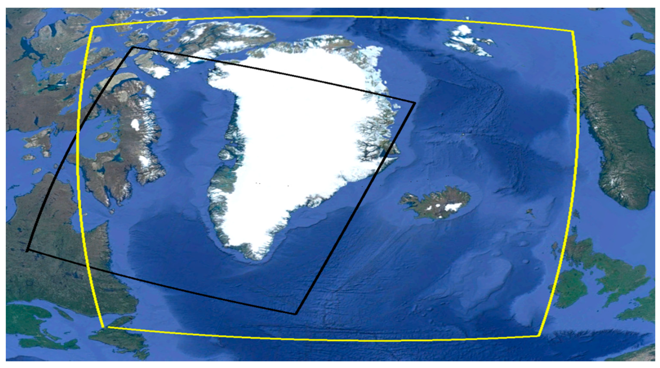
2. Field Campaigns
Numerical Models
3. The DAWN Instrument and Wind Profile Retrieval Methods
3.1. Instrument Description and Specifications
3.2. DAWN Wind Profile Retrieval
- Pointing Knowledge and Aircraft Motion Accounting—DAWN has its own GPS/INS and much effort is made to keep pointing errors below 1 degree. Navigation data from the DC-8 systems are combined with the DAWN navigation data to achieve the best results, especially with regard to well-known heading drifts.
- Utilizing Surface Returns During Calibration Legs—We use ground returns in cloud-free conditions (below aircraft) during constant altitude flight segments over uniform terrain to calibrate the GPS/INS. The attitude corrections for pitch and yaw were determined by comparing the LOS velocity at the ground for each look angle of a scan with the value of 0 m/s, which should be the speed of the ground, and iteratively finding the optimum pitch and yaw correction that minimizes the mean difference between the LOS velocities at the ground and zero. Although the correction factors derived from the ground returns should be constant once determined, we find they can vary from one day to another. The results are a significant reduction in uncertainty in the LOS wind range profiles and the vertical profiles of all three components of the winds (u, v, and w).
- Range Precision (Height Correction)—Adjusting the height assignment of range gated LOS data. The height adjustment, usually less than a few 10′s of meters, is made empirically by “correcting” the reported time of flight from the lidar system. Strong aerosol gradients just adjacent to the surface may also cause a few meters of uncertainty to the range to ground values.
4. Results
4.1. DAWN–Dropsonde Comparisons
4.2. Case Study Analyses
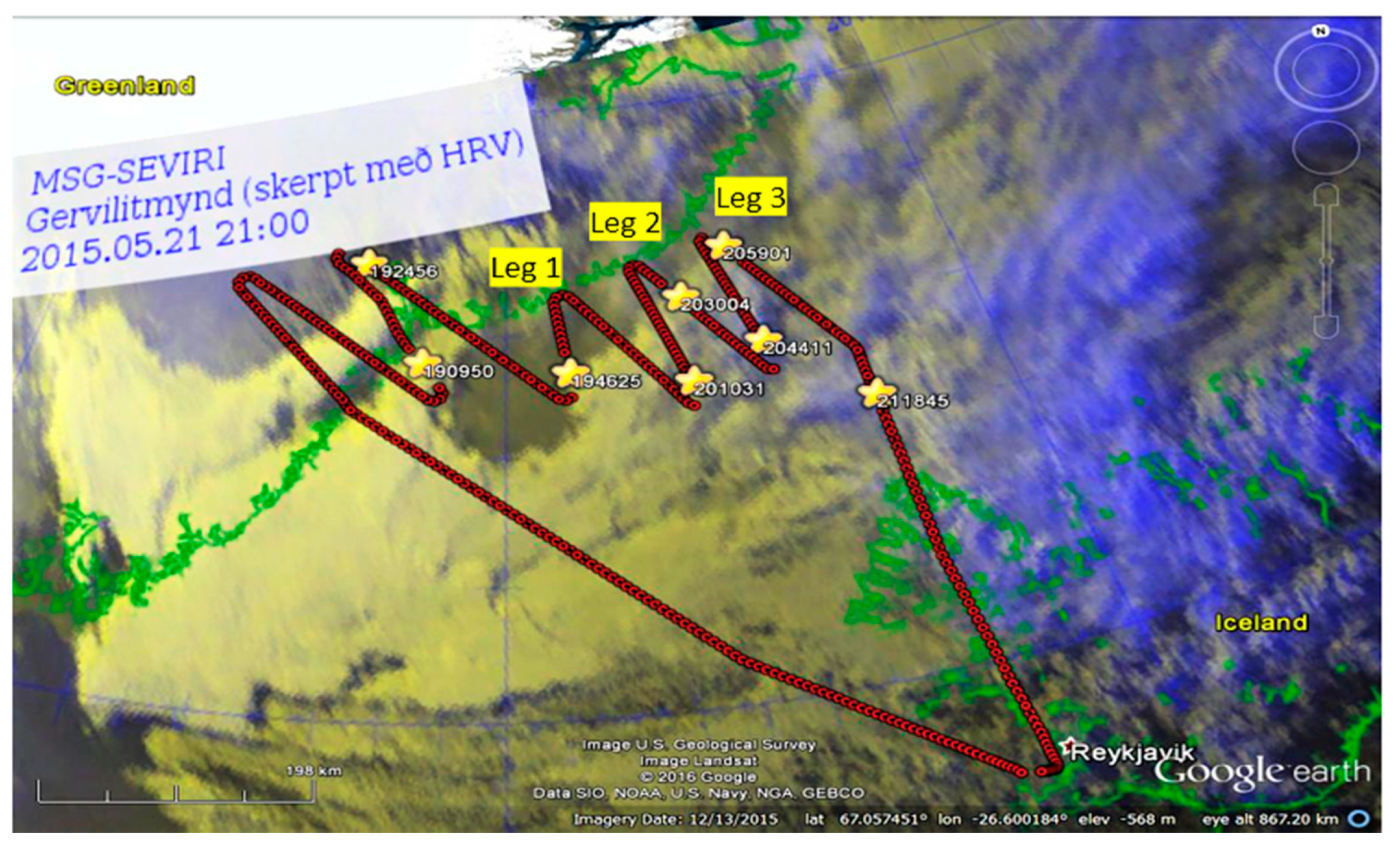
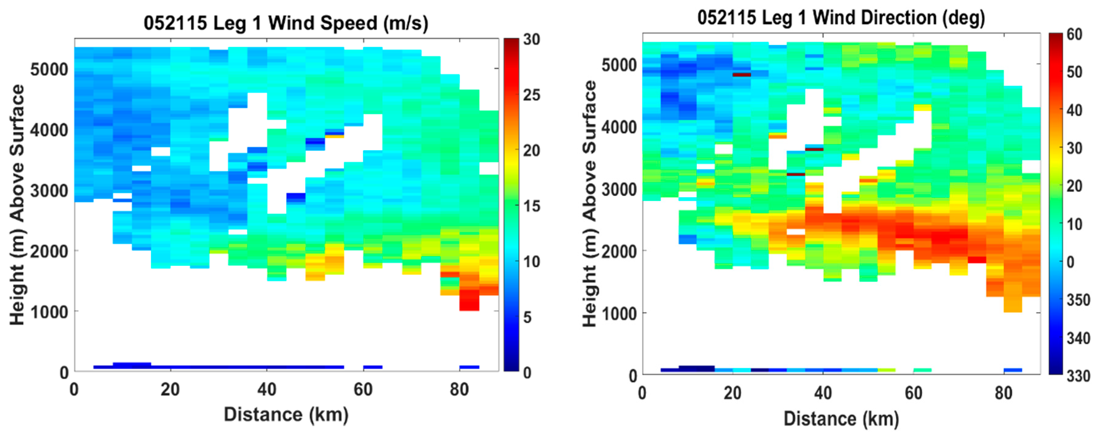
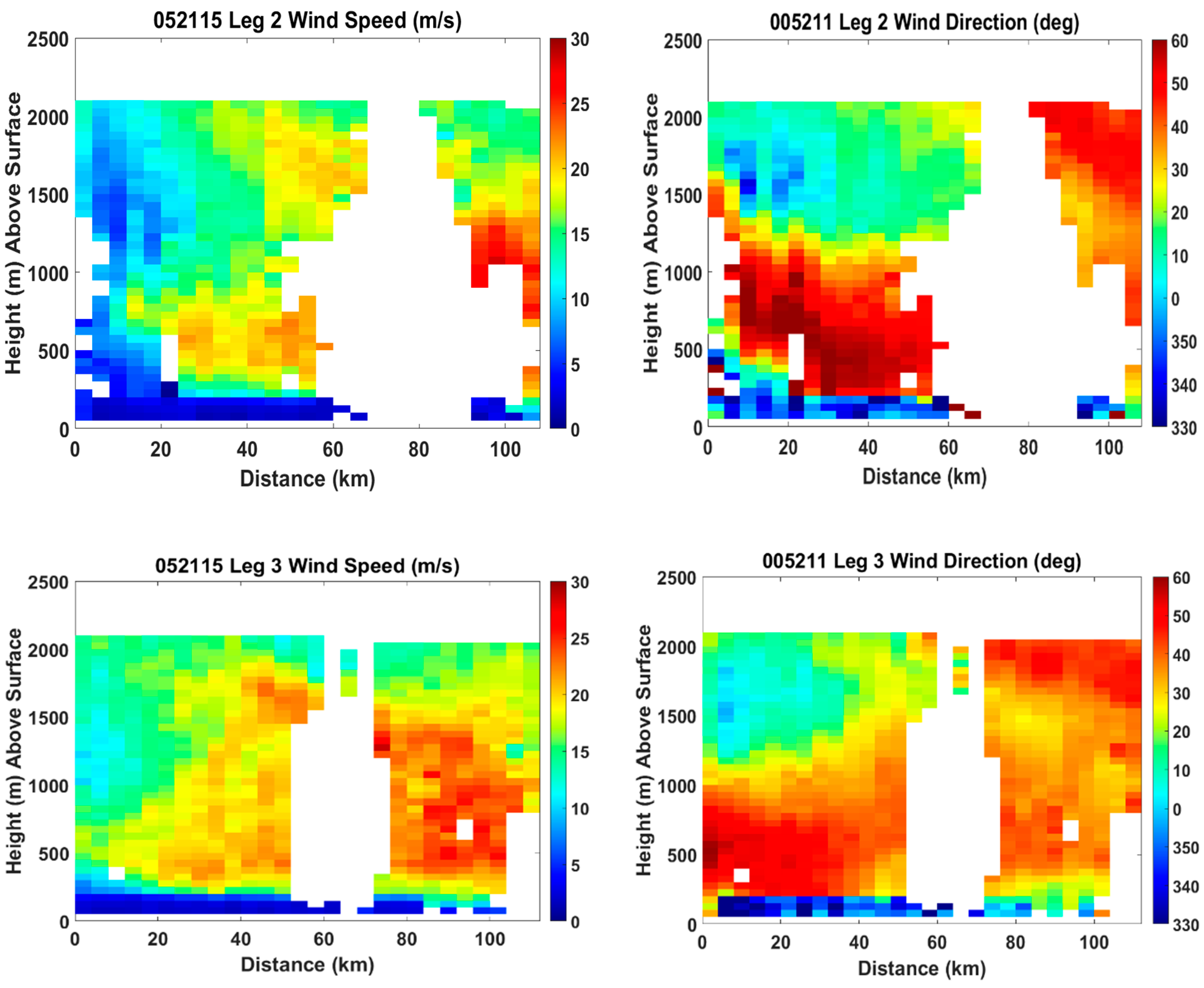
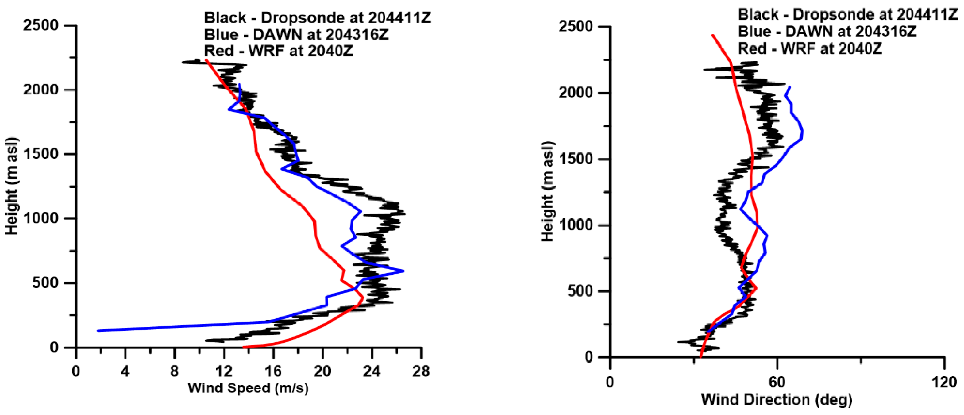
4.2.1. Barrier Wind Event during PW2 on 21 May 2015
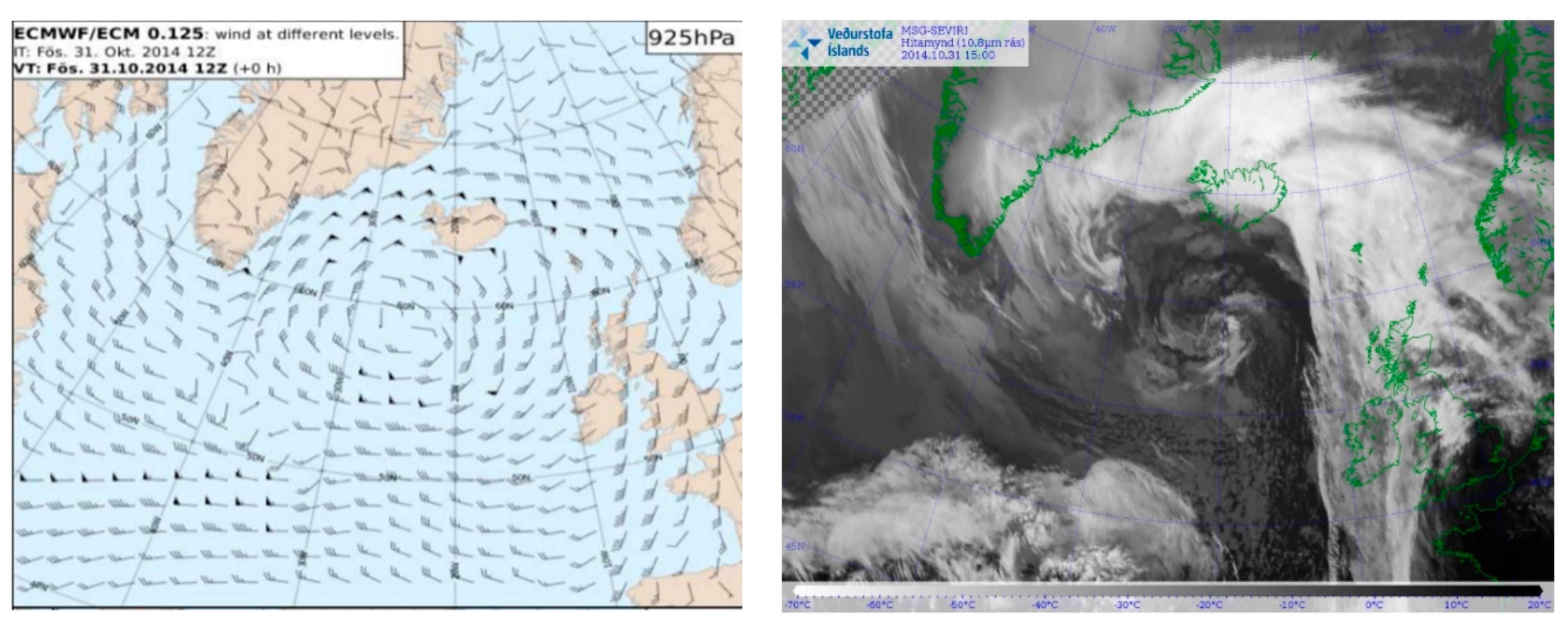
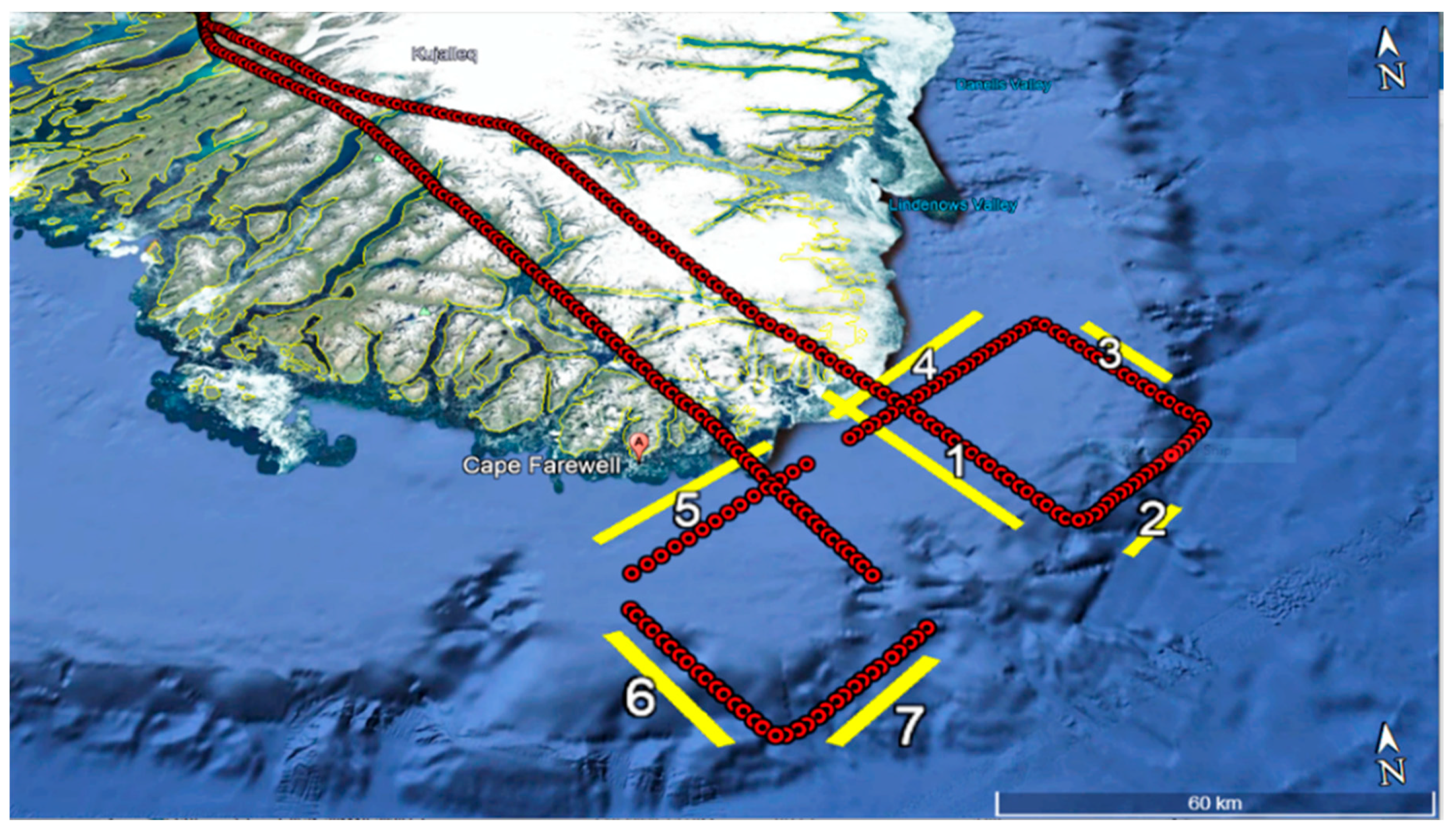
4.2.2. Greenland Tip Jet during PW1 on 31 October 2014
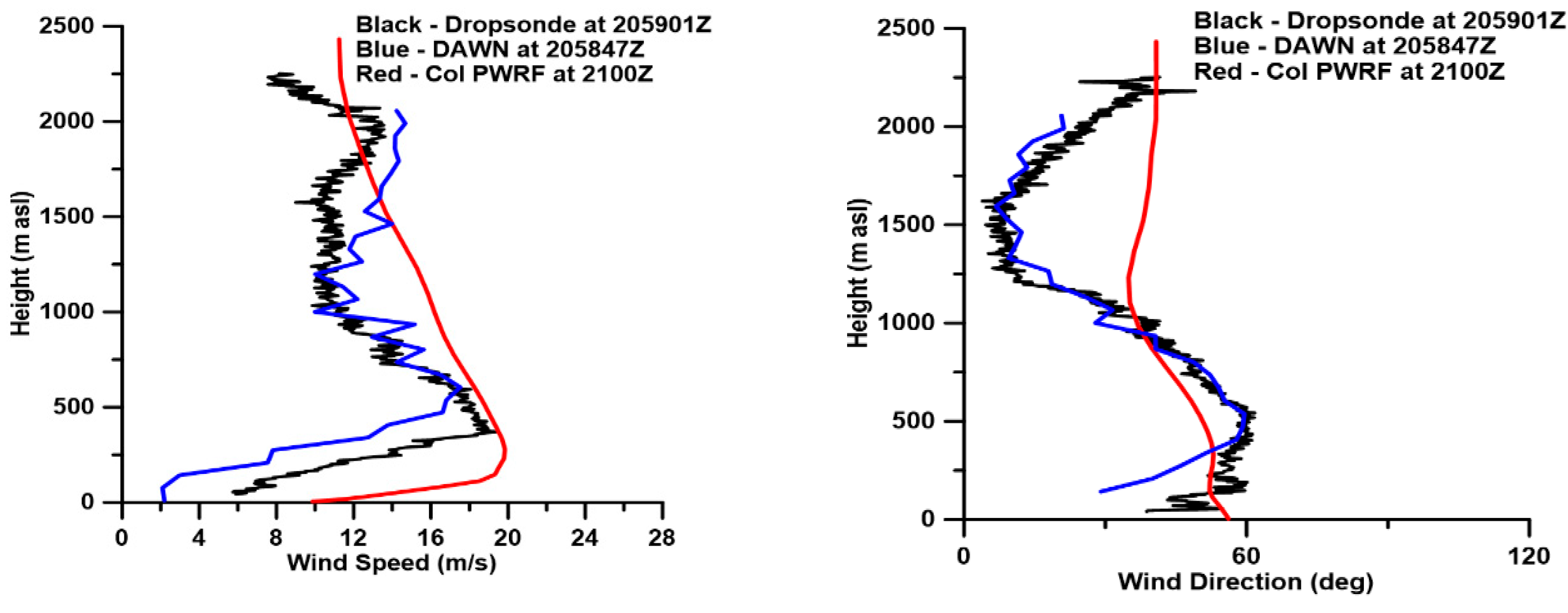
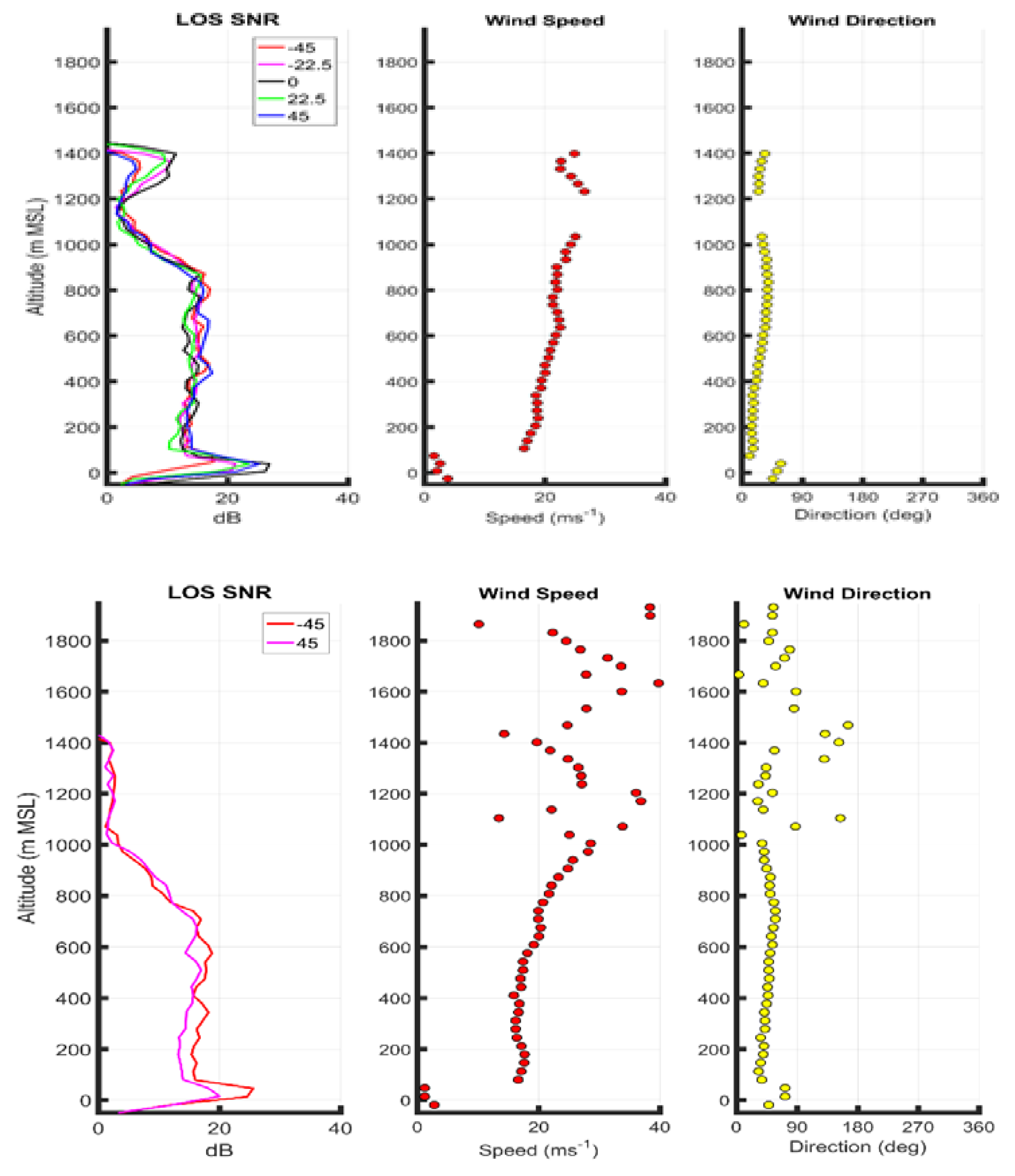
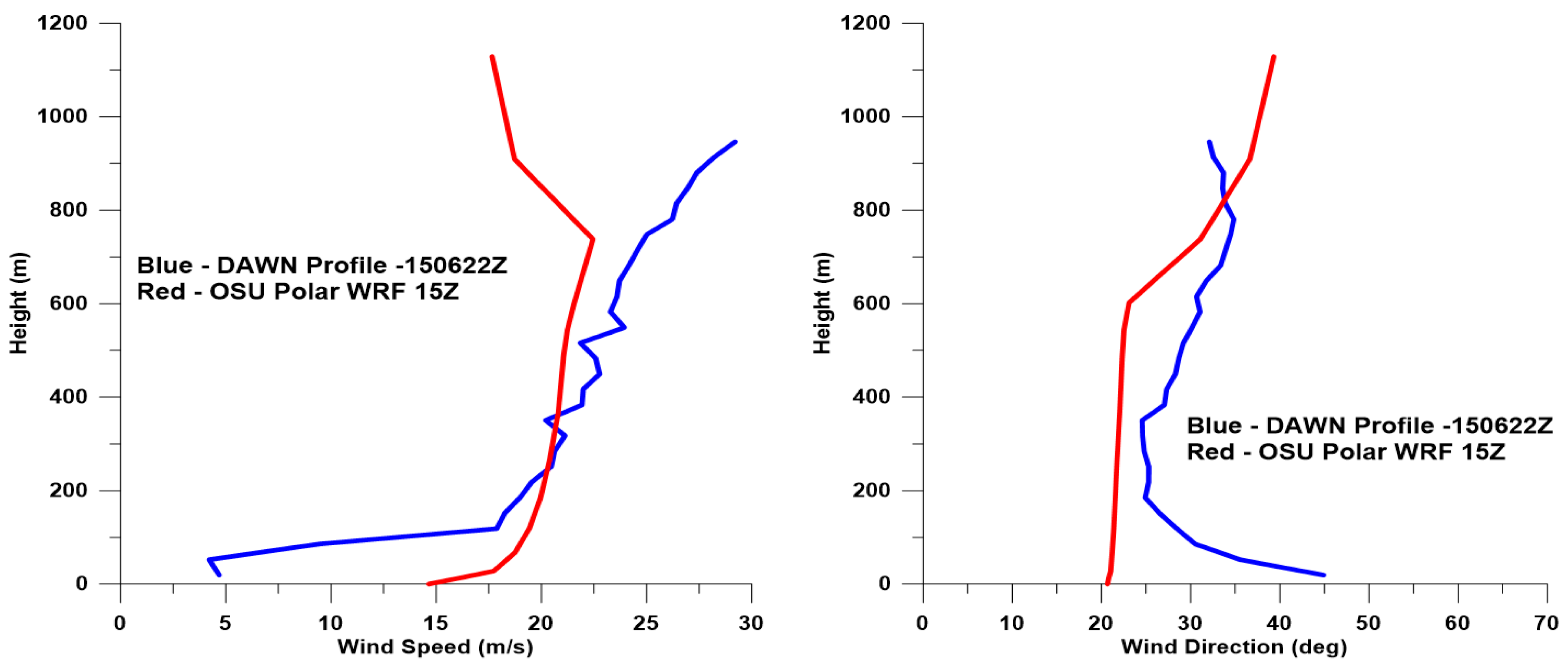
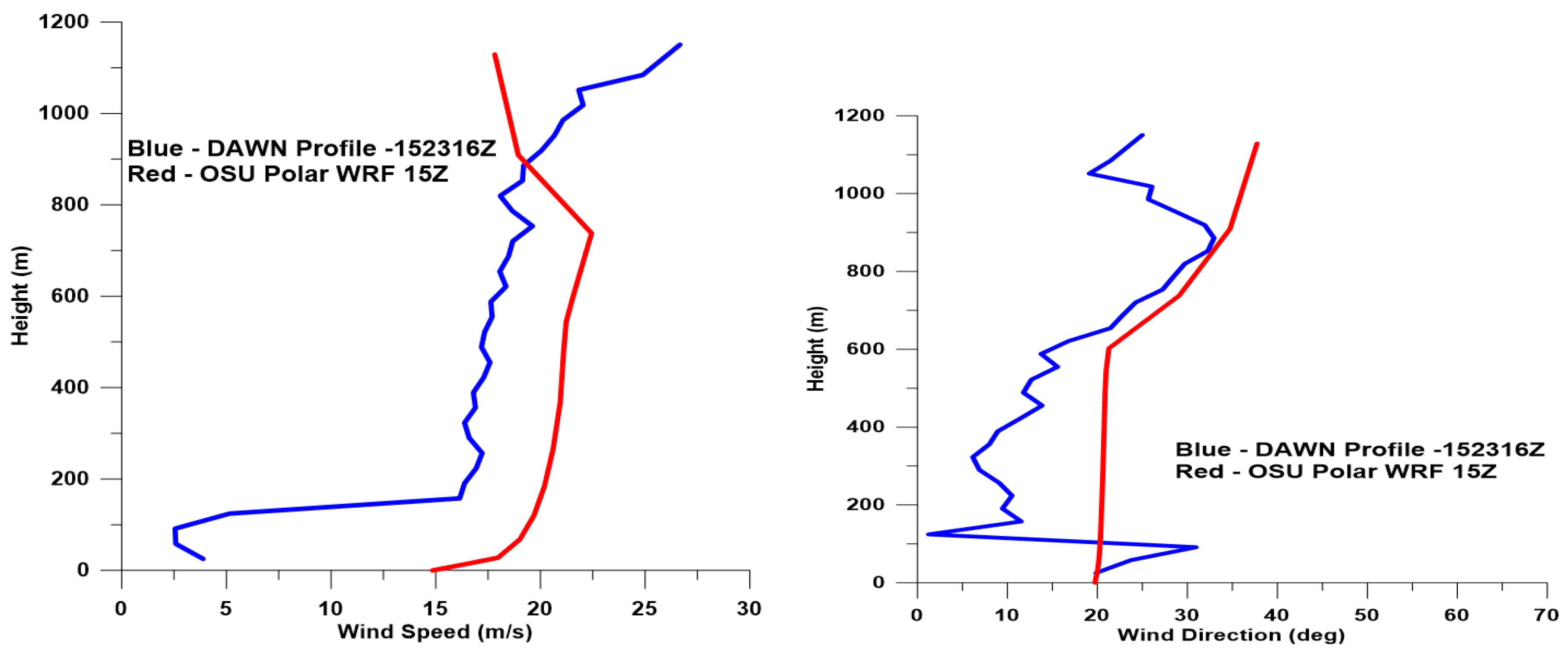
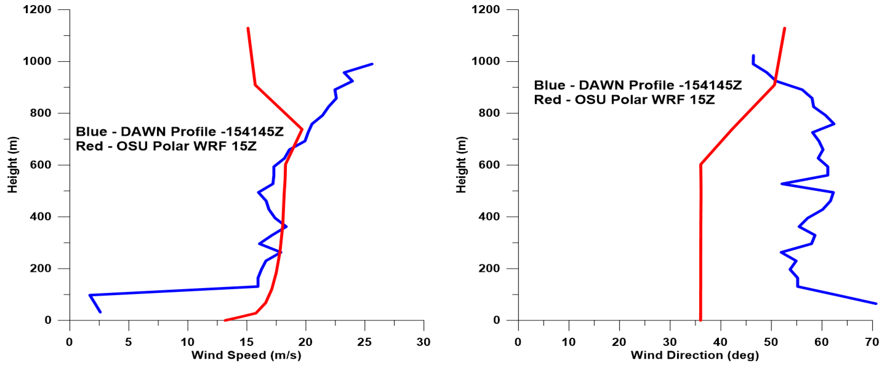
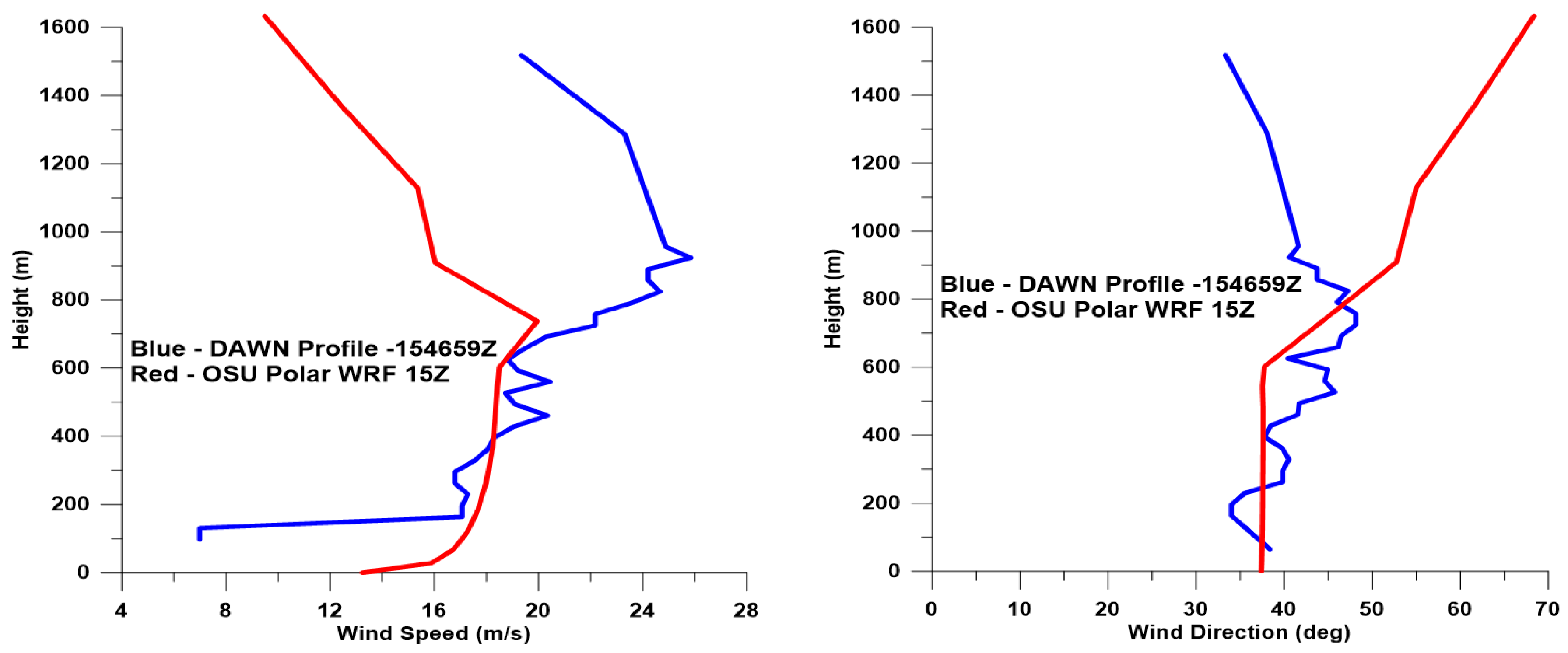
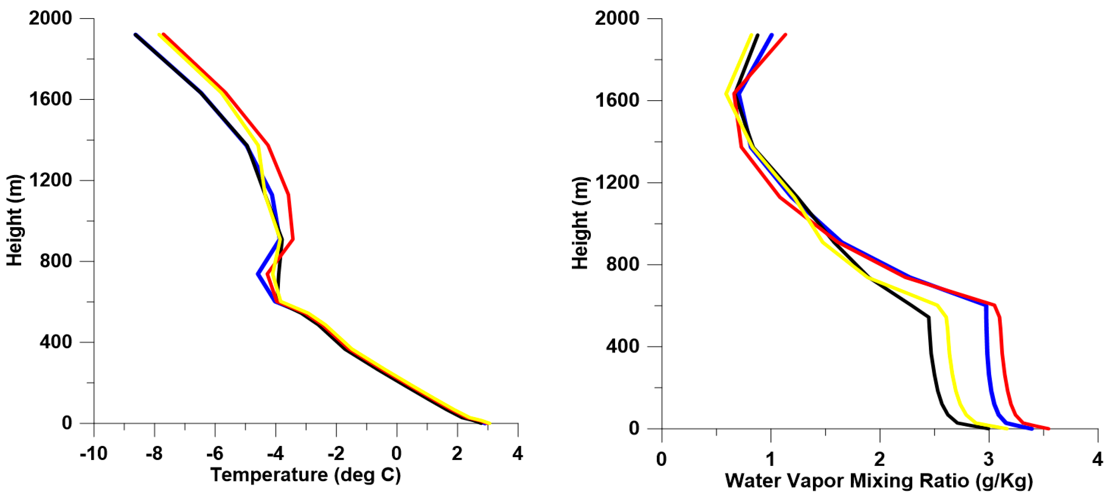
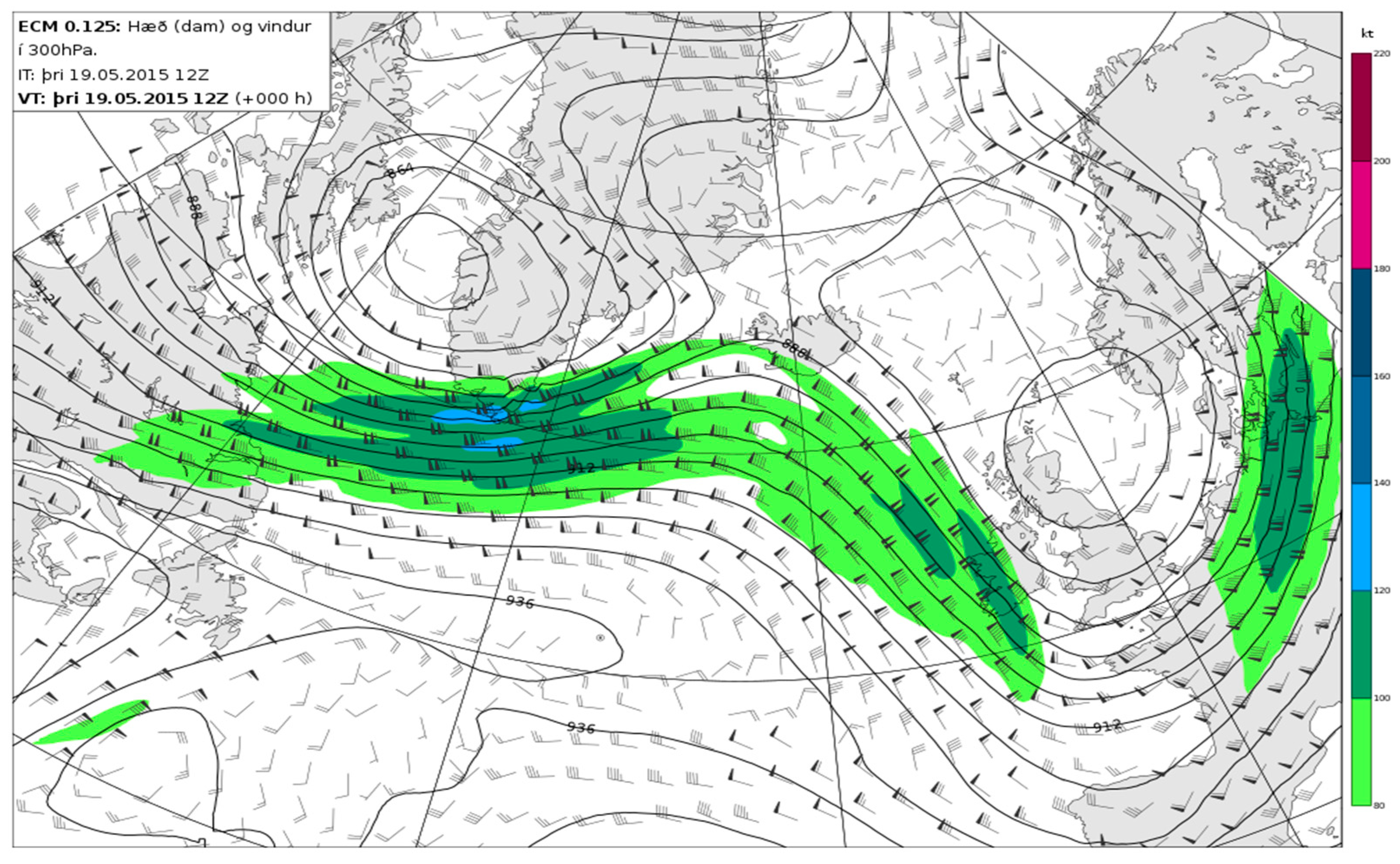
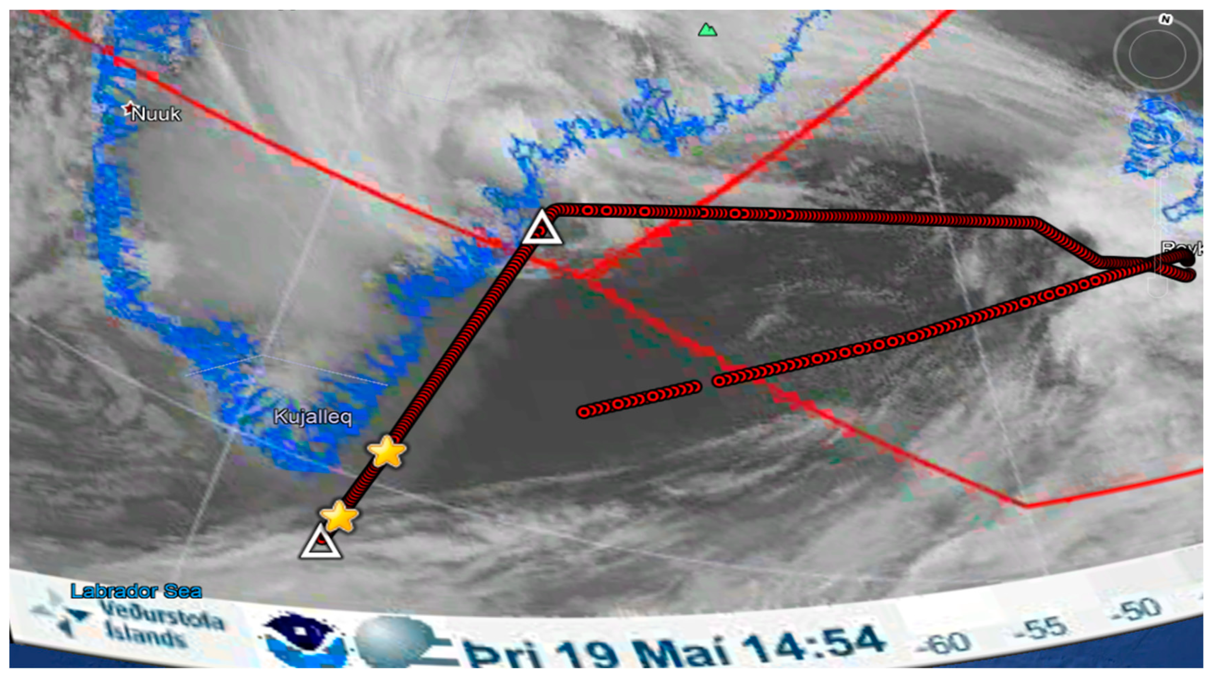
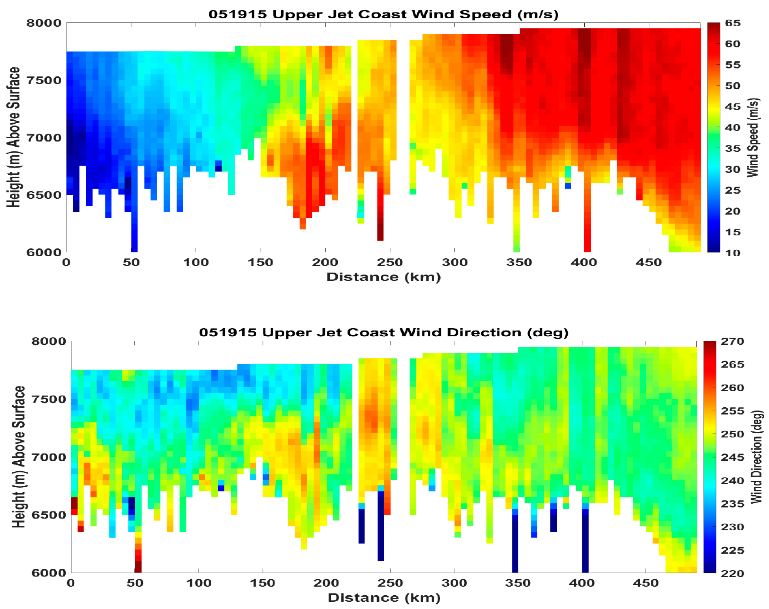
4.2.3. Upper Level Jet during PW2 on 19 May 2015
5. Discussion
- Pulse Repetition Frequency increased from 5 Hz to 10 Hz;
- Repairs to optical path (alignments, fiber connections);
- Scanner look angle options increased to include 8 and 12 looks;
- DAWN enclosure modified to allow easier access to the lidar during deployment.
6. Conclusions
Author Contributions
Funding
Acknowledgments
Conflicts of Interest
Abbreviations
| ADWL | Airborne Doppler Wind Lidar |
| ALADIN | Atmospheric Laser Doppler Instrument |
| ASCAT | Advanced Scatterometer |
| ASR | Arctic System Reanalysis |
| CALIPSO | Cloud-Aerosol Lidar and Infrared Pathfinder Satellite Observations |
| CPEX | Convective Processes Experiment |
| DAWN | Doppler Aerosol WiNd Lidar |
| DC-8 | Douglas Craft-8 |
| DLR | German Aerospace Research Establishment Deutsches Zentrum für Luft- und Raumfahrt |
| ECMWF | European Centre for Medium-Range Weather Forecasts |
| ERA | ECMWF Re-Analysis |
| FFT | Fast Fourier Transform |
| FWHM | Full Width Half Max |
| GFDex | Greenland Flow Distortion Experiment |
| GFS | Global Forecast System |
| GOES | Geostationary Operational Environmental Satellite |
| GOF | Goodness of Fit |
| GPS | Global Positioning System |
| GRIP | Genesis And Rapid Intensification Processes |
| HDSS | High Definition Sounding System |
| HLOS | Horizontal Line-of-Sight |
| HoTmLiLiF | Holmium Thulium Lutetium Lithium Fluoride |
| InGaAs | Indium Gallium Arsenide |
| INS | Inertial Navigation System |
| IPY | International Polar Year |
| LaRC | Langley Research Center |
| LM | Levenberg–Marquardt |
| LOS | Line-of-Sight |
| METEOSAT | Meteorological Satellite |
| MODIS | Moderate Resolution Imaging Spectroradiometer |
| MOSAiC | Multidisciplinary Drifting Observatory for the Study of Arctic Climate |
| MM5 | Fifth-Generation Penn State/NCAR Mesoscale Model |
| MSG | Meteosat Second Generation |
| MYJ | Mellor, Yamada, and Janjic |
| NASA | National Aeronautics and Space Administration |
| NCEP | National Center for Environmental Prediction |
| NOAA | National Oceanic and Atmospheric Administration |
| OSU | Ohio State University |
| PBL | Planetary Boundary Layer |
| P3DWL | P-3 Doppler Wind Lidar |
| PW1 | Polar Winds 1 |
| PW2 | Polar Winds 2 |
| RMSD | Root Mean Square Difference |
| RRTMG | Rapid Radiative Transfer Model for GCM |
| SEVIRI | Spinning Enhanced Visible and Infrared Imager |
| SNR | Signal to Noise Ratio |
| TCI | Tropical Cyclone Intensity |
| THORPEX | The Observing System. Research and Predictability Experiment |
| TODWL | Twin Otter Doppler Wind Lidar |
| UC-12 | Utility Cargo-12 |
| UW | University of Washington |
| WD | Wind Direction |
| WMO | World Meteorological Organization |
| WRF | Weather Research Forecast Model |
| WS | Wind Speed |
| WWRP | World Weather Research Program |
| XDD | eXpendable Digital Dropsonde |
| YES | Yankee Environmental Services |
| YOPP | Year of Polar Prediction |
| ∆WS | Wind Speed difference |
| ∆WD | Wind Direction |
| ∆Z | Height/altitude difference |
References
- Blunden, J.; Arndt, D.S. State of the Climate in 2019. Bull. Am. Meteorol. Soc. 2020, 101, Si–S429. [Google Scholar] [CrossRef]
- Achtert, P.; Brooks, I.M.; Brooks, B.J.; Moat, B.I.; Prytherch, J.; Persson, P.O.G.; Tjernström, M. Measurement of wind profiles over the Arctic Ocean from ship-borne Doppler lidar. Atmos. Meas. Tech. 2015, 8, 4993–5007. [Google Scholar] [CrossRef] [Green Version]
- Weissmann, M.; Busen, R.; Dörnbrack, A.; Rahm, S.; Reitebuch, O. Targeted observations with an airborne wind lidar. J. Atmos. Ocean. Technol. 2005, 22, 1706–1719. [Google Scholar] [CrossRef]
- Renfrew, I.A.; Petersen, G.N.; Outten, S.; Sproson, D.; Moore, G.W.K.; Hay, C.; Ohigashi, T.; Zhang, S.; Kristjánsson, J.E.; Føre, I.; et al. The Greenland flow distortion experiment. Bull. Am. Meteorol. Soc. 2008, 89, 1307–1324. [Google Scholar] [CrossRef] [Green Version]
- Kristjánsson, J.E.; Barstad, I.; Aspelien, T.; Føre, I.; Godøy, Ø.; Hov, Ø.; Irvine, E.; Iversen, T.; Kolstad, E.; Nordeng, T.E.; et al. The Norwegian IPY–THORPEX: Polar lows and Arctic fronts during the 2008 Andøya campaign. Bull. Am. Meteorol. Soc. 2011, 92, 1443–1466. [Google Scholar] [CrossRef] [Green Version]
- Wagner, J.S.; Gohm, A.; Dornbrack, A.; Schafler, A. The mesoscale structure of a polar low: Airborne lidar measurements and simulations. Q. J. R. Meteorol. Soc. 2011, 137, 1516–1531. [Google Scholar] [CrossRef] [Green Version]
- Marksteiner, U.; Reitebuch, O.; Rahm, S.; Nikolaus, I.; Lemmerz, C.; Witschas, B. Airborne direct-detection and coherent wind lidar measurements along the east coast of Greenland in 2009 supporting ESA’s Aeolus mission. In Lidar Technologies, Techniques and Measurements for Atmospheric Remote Sensing VII; International Society for Optics and Photonics: Wales, UK, 2011; Volume 8182, p. 81820. [Google Scholar]
- Marksteiner, U.; Reitebuch, O.; Lemmerz, C.; Lux, O.; Rahm, S.; Witschas, B.; Schäfler, A.; Emmitt, D.; Greco, S.; Kavaya, M.J.; et al. Airborne direct-detection and coherent wind lidar measurements over the North Atlantic in 2015 supporting ESA’s aeolus mission. In EPJ Web Conferences; EDP Sciences: Les Ulis, France, 2018; Volume 176, p. 02011. [Google Scholar]
- Marksteiner, U.; Lemmerz, C.; Lux, O.; Rahm, S.; Schäfler, A.; Witschas, B.; Reitebuch, O. Calibrations and wind observations of an airborne direct-detection wind LiDAR supporting ESA’s Aeolus mission. Remote Sens. 2018, 10, 2056. [Google Scholar] [CrossRef] [Green Version]
- Lux, O.; Lemmerz, C.; Weiler, F.; Marksteiner, U.; Witschas, B.; Rahm, S.; Schäfler, A.; Reitebuch, O. Airborne wind lidar observations over the North Atlantic in 2016 for the pre-launch validation of the satellite mission Aeolus. Atmos. Meas. Tech. 2018, 11, 3297–3322. [Google Scholar] [CrossRef] [Green Version]
- Jung, T.; Gordon, N.D.; Bauer, P.; Bromwich, D.H.; Chevallier, M.; Day, J.J.; Dawson, J.; Doblas-Reyes, F.; Fairall, C.; Goessling, H.F.; et al. Advancing polar prediction capabilities on daily to seasonal time scales. Bull. Am. Meteorol. Soc. 2016, 97, 1631–1647. [Google Scholar] [CrossRef] [Green Version]
- Shoupe, M.; de Boer, G.; Dethloff, K.; Hunke, E.; Maslowski, W.; McComiskey, A.; Perrson, O.; Randall, D.; Tjernstrom, M.; Turner, D.; et al. The Multidisciplinary Drifting Observatory for the Study of Arctic Climate (MOSAIC) Atmosphere Science Plan; DOE Office of Science Atmospheric Radiation Measurement (ARM) Program, Brookhaven National Laboratory: Upton, NY, USA, 2018.
- Dörnbrack, A.; Weissmann, M.; Rahm, S.; Simmet, R.; Reitebuch, O.; Busen, R.; Olafsson, H. Wind Lidar Observations in the Lee of Greenland. In Proceedings of the 11th Conference on Mountain Meteorology, Bartlett, NH, USA, 20–25 June 2004. [Google Scholar]
- Kavaya, M.J.; Beyon, J.Y.; Koch, G.J.; Petros, M.; Petzar, P.J.; Singh, U.N.; Trieu, B.C.; Yu, J. The Doppler Aerosol Wind Lidar (DAWN) airborne, wind-profiling, coherent-detection lidar system: Overview, flight results and plans. J. Atmos. Ocean. Technol. 2014, 34, 826. [Google Scholar] [CrossRef]
- Black, P.; Harrison, L.; Beaubien, M.; Bluth, R.; Woods, R.; Penny, A.; Smith, R.W.; Doyle, J.D. High-definition sounding system (HDSS) for atmospheric profiling. J. Atmos. Ocean. Technol. 2017, 34, 777–796. [Google Scholar] [CrossRef]
- Saha, S.; Moorthi, S.; Pan, H.L.; Wu, X.; Wang, J.; Nadiga, S.; Tripp, P.; Kistler, R.; Woollen, J.; Behringer, D.; et al. The NCEP climate forecast system reanalysis. Bull. Am. Meteorol. Soc. 2010, 91, 1015–1058. [Google Scholar] [CrossRef]
- Hersbach, H.; De Rosnay, P.; Bell, B. Operational Global Reanalysis: Progress, Future Directions and Synergies with NWP; ERA Report Series 27; European Centre for Medium Range Weather Forecasts: Reading, UK, 2018; 65p. [Google Scholar]
- Bromwich, D.H.; Wilson, A.B.; Bai, L.; Liu, Z.; Barlage, M.; Shih, C.F.; Maldonado, S.; Hines, K.M.; Wang, S.H.; Woollen, J.; et al. The Arctic system reanalysis, version 2. Bull. Am. Meteorol. Soc. 2018, 99, 805–828. [Google Scholar] [CrossRef]
- Bromwich, D.H.; Wilson, A.B.; Bai, L.; Moore, G.W.K.; Bauer, P. A comparison of the regional Arctic System Reanalysis and the global ERA-Interim reanalysis for the Arctic. Q. J. R. Meteorol. Soc. 2016, 142, 644–658. [Google Scholar] [CrossRef] [Green Version]
- Skamarock, W.C.; Klemp, J.B.; Dudhia, J.; Gill, D.O.; Barker, D.M.; Duda, M.G.; Huang, X.Y.; Wang, W.; Powers, J.G. A Description of the Advanced Research WRF Version 3, NCAR Technical Note. 2008. Available online: http://www. mmm.ucar.edu/wrf/users/docs/arw_v2 Pdf (accessed on 25 May 2015).
- Bromwich, D.H.; Hines, K.M.; Bai, L. Development and testing of Polar WRF: 2. Arctic Ocean. J. Geophys. Res. 2009, 114, D08122. [Google Scholar]
- Hines, K.M.; Bromwich, D.H.; Bai, L.; Barlage, M.; Slater, A.G. Development and testing of Polar WRF. Part III. Arctic land. J. Clim. 2011, 24, 26–48. [Google Scholar] [CrossRef] [Green Version]
- Powers, J.; Manning, K.W.; Bromwich, D.H.; Cassano, J.J.; Cayette, A.M. A decade of Antarctic science support through AMPS. Bull. Am. Meteorol. Soc. 2012, 93, 1699–1712. [Google Scholar] [CrossRef]
- DuVivier, A.K.; Cassano, J.J.; Greco, S.; Emmitt, G.D. A case study of observed and modeled barrier flow in the Denmark Strait in May 2015. Mon. Weather Rev. 2017, 145, 2385–2404. [Google Scholar] [CrossRef]
- Yu, J.; Trieu, B.C.; Modlin, E.A.; Singh, U.N.; Kavaya, M.J.; Chen, S.; Bai, Y.; Petzar, P.J.; Petros, M. 1 J/pulse Q-switched 2-micron solid-state laser. Opt. Lett. 2006, 31, 462. [Google Scholar] [CrossRef]
- Singh, U.N.; Walsh, B.M.; Yu, J.; Petros, M.; Kavaya, M.J.; Refaat, T.F.; Barnes, N.P. 20 years of Tm, Ho: YLF and LuLF laser development for global winds measurements. Opt. Mater. Express. 2015, 5, 827. [Google Scholar] [CrossRef]
- Koch, G.; Beyon, J.Y.; Cowen, L.J.; Kavaya, M.J.; Grant, M.S. Three-dimensional wind profiling of offshore wind energy areas with airborne Doppler lidar. J. Appl. Remote Sens. 2014, 8, 083662. [Google Scholar] [CrossRef]
- Koch, G.; Beyon, J.Y.; Modlin, E.A.; Petzar, P.J.; Woll, S.; Petros, M.; Yu, J.; Kavaya, M.J. Side-scan Doppler lidar for offshore wind energy applications. J. Appl. Remote Sens. 2012, 6, 063562. [Google Scholar] [CrossRef] [Green Version]
- Greco, S.; Emmitt, G.D.; Garstang, M.; Kavaya, M. Doppler Aerosol WiNd (DAWN) Lidar During CPEX 2017: Instrument performance and data utility. Remote Sens. 2020, 12, 2951. [Google Scholar] [CrossRef]
- Liu, Z.; Kavaya, M.J.; Bedka, K.M. Coherent Doppler Wind Lidar data processing software and wind retrieval from the Aeolus Cal/Val field campaign. AGUFM 2019, 2019, A12A-07. [Google Scholar]
- Doyle, J.D.; Moskaitis, J.R.; Feldmeier, J.W.; Ferek, R.J.; Beaubien, M.; Bell, M.M.; Cecil, D.L.; Creasey, R.L.; Duran, P.; Elsberry, R.L.; et al. A view of tropical cyclones from above: The tropical cyclone intensity experiment. Bull. Am. Meteorol. Soc. 2017, 98, 2113–2134. [Google Scholar] [CrossRef]
- Creasey, R.L.; Elsberry, R.L. Tropical cyclone center positions from sequences of HDSS sondes deployed along high-altitude overpasses. Weather Forecast. 2017, 32, 317–325. [Google Scholar] [CrossRef]
- Greco, S.; Emmitt, G.D.; Garstang, M.; Kavaya, M.; Pu, Z. Doppler Aerosol WiNd (DAWN) Lidar from CPEX 2017: Convective Process Studies and Comparisons with Other Wind Measurement Sensors and Numerical Models. In Proceedings of the 23rd Conference on Integrated Observing and Assimilation Systems for the Atmosphere, Oceans and Land Surface (IOAS-AOLS) Poster Session, Phoenix, AZ, USA, 8 January 2019. [Google Scholar]
- Harden, B.E.; Renfrew, I.A.; Petersen, G.N. A climatology of wintertime barrier winds off southeast Greenland. J. Clim. 2011, 24, 4701–4717. [Google Scholar] [CrossRef] [Green Version]
- Moore, G.W.K.; Renfrew, I.A. Tip jets and barrier winds: A QuikSCAT climatology of high wind speed events around Greenland. J. Clim. 2005, 18, 3713–3725. [Google Scholar] [CrossRef]
- Moore, G.W. A new look at Greenland flow distortion and its impact on barrier flow, tip jets and coastal oceanography. Geophys. Res. Lett. 2012, 39, L22806. [Google Scholar] [CrossRef]
- Moore, G.W.K.; Bromwich, D.H.; Wilson, A.B.; Renfrew, I.; Bai, L. Arctic system reanalysis improvements in topographically forced winds near Greenland. Q. J. R. Meteorol. Soc. 2016, 142, 2033–2045. [Google Scholar] [CrossRef] [Green Version]
- Renfrew, I.A.; Outten, S.D.; Moore, G.W.K. An easterly tip jet off Cape Farewell, Greenland. I: Aircraft observations. Q. J. R. Meteorol. Soc. 2009, 135, 1919–1933. [Google Scholar] [CrossRef] [Green Version]
- Doyle, J.D.; Shapiro, M.A. Flow response to large-scale topography: The Greenland tip jet. Tellus 1999, 51A, 728–748. [Google Scholar] [CrossRef] [Green Version]
- Våge, K.; Spengler, T.; Davies, H.C.; Pickart, R.S. Multi-event analysis of the westerly Greenland tip jet based upon 45 winters in ERA-40. Q. J. R. Meteorol. Soc. 2009, 135, 1999–2011. [Google Scholar] [CrossRef]
- Ohigashi, T.; Moore, K. Fine structure of a Greenland reverse tip jet: A numerical simulation. Tellus A Dyn. Meteorol. Oceanogr. 2008, 61, 512–526. [Google Scholar] [CrossRef]
- Emmitt, G.D. Advanced processing of Airborne Doppler Wind Lidar wind measurements to resolve PBL circulations and near surface wind fields over the open ocean. In Proceedings of the AGU 100th Fall Meeting, A41L—Boundary Layer Clouds and Turbulence and Their Interaction with the Underlying Land or Ocean Surface Poster Session, San Francisco, CA, USA, 12 December 2019. [Google Scholar]


| Mission Number | Date | Time (GMT) | Science Objectives |
|---|---|---|---|
| 1 | 10/29/14 | 1151–1347 | Ice–land–water boundary layer |
| 2 | 10/29/14 | 1456–1643 | CALIPSO underflight; Marine boundary layer |
| 3 | 10/30/14 | 1323–1642 | Land–water; west coast of Greenland; Aeolus simulation |
| 4 | 10/31/14 | 1101–1919 | Tip jet; Land–ice cap transect; Aeolus simulation |
| 5 | 11/3/14 | 1356–1714 | Offshore transects; CALIPSO/ASCAT underflight |
| 6 | 11/4/14 | 1358–1727 | Land–water boundary layer; Aeolus simulation; MODIS underflight |
| 7 | 11/5/14 | 1411–1721 | Land–ice cap edge; Cloud layers |
| 8 | 11/6/14 | 1405–1631 | Marine boundary layer; Aeolus simulation; MODIS underflight |
| 9 | 11/7/14 | 1411–1648 | Boundary layer (land–water) |
| 10 | 11/8/14 | 1554–1913 | Coastal katabatic flow; MODIS/ASCAT underflight |
| 11 | 11/10/14 | 1428–1700 | Coastal boundary layer (rolls); CALIPSO/ASCAT underflight |
| 12 | 11/11/14 | 1407–1717 | Land–marine boundary layer |
| 13 | 11/12/14 | 1106–1854 | Tip jet/winds; off-shore transect |
| 14 | 11/13/14 | 1403–1625 | All land/ice cap boundary layer |
| Mission Number | Date | Time (GMT) | Science Objectives |
|---|---|---|---|
| 1 | 5/11/15 | 1318–1720 | Around Iceland |
| 2 | 5/13/15 * | 1057–1503 | TechDemoSat 1 underpass |
| 3 | 5/15/15 * | 1604–2006 | North Atlantic upper jet stream |
| 4 | 5/16/15 * | 1357–2106 | Aeolus cal/val flight; southern Greenland |
| 5 | 5/17/15 | 1352–2109 | Tip jet and katabatic flow off east coast of Greenland |
| 6 | 5/19/15 * | 1200–1702 | Tip jet, Coastal upper jet; Aeolus cal/val flight |
| 7 | 5/21/15 | 1742–2151 | Barrier winds |
| 8 | 5/23/15 * | 1354–1955 | Southeast coast of Greenland; ice, land and water transects Aeolus cal/val flight |
| 9 | 5/24/15 | 1153–1822 | Coastal zone off west coast of Greenland |
| 10 | 5/25/15 * | 1407–1716 | Around Iceland; Upper jet; Aeolus cal/val flight |
| WRF Scheme/Feature | OSU Polar WRF PW1/PW2 | WRF Version 3.7.1 PW2 |
|---|---|---|
| Initialization Time | Twice daily (00Z/12Z) | 00Z |
| Boundary Conditions | NCEP GFS (28 km) | ECMWF ERA-I (70 km) |
| Horizontal Resolution | 8 km | 5 km |
| Vertical Levels | 49 | 60 |
| Sea Ice Thickness | 1.5 m | 0.5 m |
| Longwave Radiation | RRTMG | RRTMG |
| Shortwave Radiation | RRTMG | RRTMG |
| Cumulus Param. | Grell-3 | Kain–Fritsch |
| Microphysics | Morrison | Morrison |
| Surface Layer | MYJ | Revised MM5 |
| Land Surface Model | Noah | Noah |
| Planetary Boundary Layer Scheme | MYJ | UW |
| Attribute | Value |
|---|---|
| Airplanes flown | DC-8 and UC-12B |
| Solid-state laser crystal and wavelength | Holmium Thulium Lutetium Lithium Fluoride (Ho:Tm:LuLiF), 2.053472 microns |
| Laser pulse energy, rate, and Full Width Half Max (FWHM) duration | 250 mJ, 10 Hz, 180 ns (PW1); 100 mJ, 5 Hz, 180 ns (PW2) |
| Number of LOS/azimuth angles | Selectable; Only 2 and 5 angles used |
| Number of laser shots at each LOS | Selectable, typically 10–20 (1–2 s) |
| Optical detection | Dual-balanced coherent (heterodyne), Indium Gallium Arsenide (InGaAs) |
| Laser pointing knowledge | Dedicated Inertial Navigation System (INS)/Global Positioning System (GPS) on lidar supplemented with ground returns |
| Horizontal Resolution of Vertical Profile | 3–10 km |
| Vertical Resolution of Vertical Profile | 66 m |
| LOS wind measurement precision | <1 m/s |
| u, v, w measurement precision | <1 m/s |
| Data product vertical resolution | 75–150 m typical, selectable |
| Horizontal resolution of each LOS wind profile | 500 m typical (variable with # shots) |
| Horizontal resolution of vertical profile of horizontal wind | 3–12 km typ. (variable with # LOS, #shots, aircraft ground speed) |
| Height Layer | Number of Comparisons | ∆z (m) | Mean ∆WS (Bias) | RMSD ∆WS | Mean ∆WD (Bias) | RMSD ∆WD |
|---|---|---|---|---|---|---|
| ALL | 2548 | 2.28 | −0.01 | 1.98 | −0.48 | 15.9 |
| 0–2.5 km | 430 | 1.94 | 0.09 | 1.99 | −0.48 | 18.0 |
| 2.5–5 km | 812 | 2.00 | 0.48 | 1.23 | −1.75 | 22.7 |
| 5.0–7.5 km | 710 | 2.48 | −0.14 | 1.85 | −0.51 | 9.27 |
| Above 7.5 km | 596 | 2.64 | −0.58 | 2.04 | 0.91 | 6.50 |
| Wind Speed Range | Number of Comparisons | ∆z (m) | Mean ∆WS (Bias) | RMSD ∆WS | Mean ∆WD (Bias) | RMSD ∆WD |
| ALL | 2548 | 2.28 | −0.01 | 1.98 | −0.48 | 15.9 |
| 0–10 m/s | 826 | 1.98 | 0.05 | 1.74 | 1.11 | 22.5 |
| 10–20 m/s | 777 | 2.21 | 0.23 | 1.97 | −2.40 | 10.3 |
| 20–30 m/s | 452 | 2.64 | −0.45 | 2.25 | −0.23 | 6.25 |
| Over 30 m/s | 493 | 2.53 | −0.08 | 2.06 | 0.32 | 1.68 |
Publisher’s Note: MDPI stays neutral with regard to jurisdictional claims in published maps and institutional affiliations. |
© 2020 by the authors. Licensee MDPI, Basel, Switzerland. This article is an open access article distributed under the terms and conditions of the Creative Commons Attribution (CC BY) license (http://creativecommons.org/licenses/by/4.0/).
Share and Cite
Greco, S.; Emmitt, G.D.; DuVivier, A.; Hines, K.; Kavaya, M. Polar Winds: Airborne Doppler Wind Lidar Missions in the Arctic for Atmospheric Observations and Numerical Model Comparisons. Atmosphere 2020, 11, 1141. https://doi.org/10.3390/atmos11111141
Greco S, Emmitt GD, DuVivier A, Hines K, Kavaya M. Polar Winds: Airborne Doppler Wind Lidar Missions in the Arctic for Atmospheric Observations and Numerical Model Comparisons. Atmosphere. 2020; 11(11):1141. https://doi.org/10.3390/atmos11111141
Chicago/Turabian StyleGreco, Steven, George D. Emmitt, Alice DuVivier, Keith Hines, and Michael Kavaya. 2020. "Polar Winds: Airborne Doppler Wind Lidar Missions in the Arctic for Atmospheric Observations and Numerical Model Comparisons" Atmosphere 11, no. 11: 1141. https://doi.org/10.3390/atmos11111141
APA StyleGreco, S., Emmitt, G. D., DuVivier, A., Hines, K., & Kavaya, M. (2020). Polar Winds: Airborne Doppler Wind Lidar Missions in the Arctic for Atmospheric Observations and Numerical Model Comparisons. Atmosphere, 11(11), 1141. https://doi.org/10.3390/atmos11111141