Insight into Construction of Tikhonov-Type Regularization for Atmospheric Retrievals

Abstract

In atmospheric science we are confronted with inverse problems arising in applications associated with retrievals of geophysical parameters. A nonlinear mapping from geophysical quantities (e.g., atmospheric properties) to spectral measurements can be represented by a forward model. An inversion often suffers from the lack of stability and its stabilization introduced by proper approaches, however, can be treated with sufficient generality. In principle, regularization can enforce uniqueness of the solution when additional information is incorporated into the inversion process. In this paper, we analyze different forms of the regularization matrix $\mathbf{L}$ in the framework of Tikhonov regularization: the identity matrix ${\mathbf{L}}_0$, discrete approximations of the first and second order derivative operators ${\mathbf{L}}_1$ and ${\mathbf{L}}_2$, respectively, and the Cholesky factor of the a priori profile covariance matrix ${\mathbf{L}}_{\mathrm{C}}$. Each form of $\mathbf{L}$ has its intrinsic pro/cons and thus may lead to different performance of inverse algorithms. An extensive comparison of different matrices is conducted with two applications using synthetic data from airborne and satellite sensors: retrieving atmospheric temperature profiles from microwave spectral measurements, and deriving aerosol properties from near infrared spectral measurements. The regularized solution obtained with ${\mathbf{L}}_0$ possesses a reasonable magnitude, but its smoothness is not always assured. The retrieval using ${\mathbf{L}}_1$ and ${\mathbf{L}}_2$ produces a solution in favor of the smoothness, and the impact of the a priori knowledge is less critical on the retrieval using ${\mathbf{L}}_1$. The retrieval performance of ${\mathbf{L}}_{\mathrm{C}}$ is affected by the accuracy of the a priori knowledge.

1. Introduction

An inverse problem is the process of using a given set of data to infer the parameters in a model that can characterize the given data. Rank-deficiency (insufficient information contained in the given data) and ill-posedness (no solution or a non-unique solution, and/or an unstable solution procedure) are often encountered when dealing with practical inverse problems in science and engineering, e.g., astronomy, geophysics, remote sensing, signal processing, etc. Both situations are characterized by a function which is ill-conditioned, i.e., the condition number of this function is very large. This leads to the primary difficulty that these inverse problems are practically underdetermined. Therefore, it is essential to incorporate additional information about the desired solution in order to stabilize the problem-solving process and to obtain a meaningful solution.

A representative example of an ill-posed problem is the Fredholm integral equation of the first kind that establishes a linear relationship between the known function g consisting of measured quantities and the unknown function f:

$${\int }_0^{1}K(s,t)f\left(t\right)\mathrm{d}t=g\left(s\right),with0\le s\le 1,$$

(1)

where the kernel K represents the underlying model that describes the relationship between g and f. To solve such problems, discretization is often needed to obtain a numerical solution. The so-called Picard condition [1,2] puts requirements on the right-hand term g so that the solution f is square integrable. As a matter of fact, the solution f is extremely sensitive to perturbations of the right-hand term g, i.e., even a very small random perturbation to g may result in a significant deviation in f, and in this sense the inverse problem of inferring f from g is ill-posed.

In atmospheric science, solving an inverse problem is a process of estimating geophysical quantities based on a given set of spectral measurements recorded by an instrument on various platforms [3,4,5]. A retrieval is often done by iteratively adjusting atmospheric state parameters associated with radiative transfer to mimic those spectral measurements; however, the atmospheric radiative transfer modeling can be a challenging task, since a number of assumptions have to be made and the computational process needs to be optimized using different numerical approaches [6,7,8].

The radiative transfer model cannot be inverted analytically. Instead, the inverse problem is an exercise in optimization, i.e., minimization of an objective function. A physically meaningful solution could be difficult to find because the governing equations tend to be mathematically ill-posed. The regularization procedure aims to stabilize the solution-finding process by introducing additional information into the objective function. In many numerical regularization methods, this is achieved by adding a term with constraints (so-called penalty term), such as restrictions for smoothness or bounds on the normed vector space (see Section 2.2 for mathematical expressions). Modern and sophisticated regularization approaches for computing regularized solutions to inverse problems in geoscience can be found in a number of textbooks, e.g., [1,9,10,11,12].

The majority of deployed retrieval algorithms use classical methods e.g., Tikhonov regularization (TR) approaches [13,14], and statistical methods based on Bayes’ theorem [15], e.g., the optimal estimation method (OEM) [5]. The principle difference between OEM and TR is the formulation of the penalty term: OEM introduces the statistical information of natural variability, whereas TR enforces the smoothness and/or impacts the magnitude of the solution. Eriksson [16] compared both methods theoretically and discovered no fundamental differences in the retrieval output. However, to find an optimal regularized solution to the underlying problem, the penalty term needs to be properly constructed.

The regularization used in atmospheric retrievals (of trace gas concentrations, temperature, etc.) reduces the noise effect with a cost in the reduction in effective resolution in terms of degrees of freedom for signal. TR-based methods need to deal with the selection of a proper regularization parameter which is frequently done on an ad hoc basis. Typical parameter selection approaches were outlined in [17,18]. Recently, new methods for satellite retrievals were proposed in [19,20]. Additionally, Koner and Drummond [21] analyzed the impact of the regularization strength using the regularized trust-region method.

The major objective of this study is to address the impact of the penalty term on the retrieval outcome using TR-based methods and to explore appropriate strategies in coping with different retrieval problems. This topic has not been heavily discussed, as in atmospheric remote sensing OEM has become a standard retrieval method by taking into account an estimate of the covariances associated with the spectral measurements and parameters of interest. Few studies focused on the choice of regularization matrix from a practical point of view. This study is accordingly intended to offer potential solutions to these problems.

This paper is based on an analysis of the numerical performance of the TR-based retrieval methods with applications to the estimation of atmospheric properties. The main focus is on the regularization matrix and its impact on the retrieval outcome. The remainder of this paper is structured as follows: Section 2 presents theoretical concepts addressing forward and inverse problems in atmospheric remote sensing, for a TR-based inversion framework various designs of the regularization matrix are specifically described. In Section 3, the numerical performance of solving ill-posed inverse problems using different regularization matrices is investigated based on retrievals of temperature profiles and aerosol properties from an airborne microwave radiometer and a satellite hyperspectral sensor, respectively. Section 4 concludes with a summary of our findings.

2. Theory

This section deals with the theoretical concepts underlying atmospheric inversion. As an application of physics-based inversion algorithms, a retrieval of atmospheric state typically requires inverting the radiative transfer equation to derive geophysical variables of interest from spectral measurements.

2.1. Forward Problem

The attenuation of radiation through the atmosphere $\mathrm{d}I$ is proportional to the incoming radiation, the differential path distance $\mathrm{d}s$ in the direction Ω, and the composition of the atmospheric medium. The radiation detected by a sensor is described by the theory of radiative transfer. Generally, the radiative transfer equation can be formulated as:

$$\frac{1}{{\sigma }_{\mathrm{ext}}\left(r\right)}\frac{\mathrm{d}I}{\mathrm{d}s}(r,\mathrm{\Omega })=I(r,\mathrm{\Omega })+J(r,\mathrm{\Omega }),$$

(2)

where $I(r,\mathrm{\Omega })$ is the diffuse radiance at position $r$ and in the direction $\mathrm{\Omega }=(\mu ,\theta )$ characterized by the cosine of the zenith angle $\mu$ and the azimuth angle $\theta$, ${\sigma }_{\mathrm{ext}}\left(r\right)$ is the extinction coefficient, $J(r,\mathrm{\Omega })$ is the source function.

For practical purposes, the radiative transfer can be treated with different techniques in different spectral regions: it is justified to neglect the thermal emission across the ultraviolet (UV), visible (VIS), and near infrared (NIR), while the scattering processes are usually neglected or simplified in the IR/microwave. Extensive discussions of the radiative transfer theory can be found in many textbooks, e.g., [22,23,24,25,26].

2.1.1. Radiative Transfer in the UV–VIS–NIR

A common way to compute the diffuse radiance in a spherical shell atmosphere is the pseudo-spherical model [27] that treats the multiple scattering in a plane-parallel atmosphere and the solar beam attenuation in a curved atmosphere. Thus, we have ${\sigma }_{\mathrm{ext}}\left(r\right)={\sigma }_{\mathrm{ext}}\left(r\right)$ and $I(r,\mathrm{\Omega })=I(r,\mathrm{\Omega })$, Equation (2) is then rewritten as

$$\mu \frac{\mathrm{d}I}{\mathrm{d}r}(r,\mathrm{\Omega })=-{\sigma }_{\mathrm{ext}}\left(r\right)I(r,\mathrm{\Omega })+J_{\mathrm{ss}}+J_{\mathrm{ms}},$$

(3)

where the single and multiple scattering source terms are computed by

$$J_{\mathrm{ss}}=F_{\mathrm{sun}}\frac{{\sigma }_{\mathrm{sct}}\left(r\right)}{4\pi }p(r,\mathrm{\Omega },{\mathrm{\Omega }}_{\mathrm{sun}}){\mathrm{e}}^{-{\tau }_{\mathrm{ext}}^{\mathrm{sun}}(r,r_{\mathrm{TOA}})}$$

(4)

and

$$J_{\mathrm{ms}}=\frac{{\sigma }_{\mathrm{sct}}\left(r\right)}{4\pi }{\int }_{4\pi }p(r,\mathrm{\Omega },{\mathrm{\Omega }}^{\prime })I(r,{\mathrm{\Omega }}^{\prime })\mathrm{d}{\mathrm{\Omega }}^{\prime },$$

(5)

respectively. ${\sigma }_{\mathrm{ext}}$ and ${\sigma }_{\mathrm{sct}}$ are the extinction and scattering coefficients (of gas molecules and aerosols), respectively; $F_{\mathrm{sun}}$ stands for the solar irradiance at the top of atmosphere (TOA) before attenuation by the atmospheric medium; the incident solar direction is defined as ${\mathrm{\Omega }}_{\mathrm{sun}}=(-{\mu }_{\mathrm{sun}},{\theta }_{\mathrm{sun}})$ with ${\mu }_{\mathrm{sun}}>0$; ${\tau }_{\mathrm{ext}}^{\mathrm{sun}}(r,r_{\mathrm{TOA}})$ is the solar optical depth between point $r$ and $r_{\mathrm{TOA}}$; $p(r,\mathrm{\Omega },{\mathrm{\Omega }}^{\prime })$ is the effective scattering phase function with $\mathrm{\Omega }$ and ${\mathrm{\Omega }}^{\prime }$ being unit vector specifying the incident and scattering directions, respectively. Note that the thermal emission is neglected in this spectral domain.

The dependence of p on the angle $\mathrm{\Theta }$ between the incident and scattering directions allows for an expansion in terms of normalized Legendre functions $P_n$:

$$p(r,\mathrm{\Omega },{\mathrm{\Omega }}^{\prime })=\sum _{n=0}^{}\sqrt{\frac{2n+1}{2}}{\chi }_n\left(r\right)P_n(cos\mathrm{\Theta }),$$

(6)

where $cos\mathrm{\Theta }=\mathrm{\Omega }·{\mathrm{\Omega }}^{\prime }$. p needs to take into account Rayleigh scattering by molecules (small particles) and Mie scattering by aerosols (large particles). Aerosol microphysical properties need to be taken into account and can be extracted from an aerosol model with a set of aerosol types.

In practice, the discrete ordinate approach [28,29,30] has been widely employed to determine the solution to the radiative transfer equation. In particular, the range of zenith angles $\mu$ is divided to a number of discrete angular intervals, and I and p are replaced by a discrete set of direction vectors. By using the matrix exponential technique in [31] or the eigenvalue approach in [30], the integral in Equation (5) becomes then a sum, while the radiative transfer equation is converted into a set of coupled linear ordinary differential equations that are later equipped with corresponding boundary conditions.

2.1.2. Radiative Transfer in the IR/Microwave

In the IR and microwave spectral range, assuming a non-scattering medium in the state of local thermodynamic equilibrium (LTE), the radiance I at frequency f received by an instrument at position $r$ can be represented by the Schwarzschild equation:

$$I(f;r)=I(f;r_{\mathrm{s}})\mathcal{T}(f;r,r_{\mathrm{s}})+{\int }_{|r-r_{\mathrm{s}}|}B(f,T\left(r^{\prime }\right))\frac{\partial \mathcal{T}}{\partial s}(f;r,r^{\prime })\mathrm{d}s,$$

(7)

where $I(f;r_{\mathrm{s}})$ is the background contribution at position $r_{\mathrm{s}}$, and $B(f,T(s\left)\right)$ is the Planck function at temperature T. $\mathcal{T}$ stands for the monochromatic transmission and is computed via

$$\mathcal{T}(f;r,r_{\mathrm{s}})={\mathrm{e}}^{-\tau (f;r,r_{\mathrm{s}})}=exp\left[-{\int }_r^{r_{\mathrm{s}}}{\sigma }_{\mathrm{abs}}(f,s^{\prime })\mathrm{d}{s}^{\prime }\right].$$

(8)

A simulation of high-resolution spectroscopic measurements usually requires line-by-line computations. The absorption coefficient ${\sigma }_{\mathrm{abs}}$ is determined by the product of molecular absorption cross sections and number densities summed over the molecules; the absorption cross section k for each line l is obtained by summing over the contributions from many lines:

$${\sigma }_{\mathrm{abs}}(f,r)=\sum _m{k}_m(f;p,T)n_m=\sum _m\sum _l{S}_l\left(T\right)g\left(f;f_l^,{\gamma }_l(p,T)\right),$$

(9)

where $S_l\left(T\right)$, g, and $f_l$ represent the line strength at temperature T, a normalized line shape function, and central frequency of transition l, respectively.

The monochromatic frequency/wavenumber grid point spacing related to the half-widths of the spectral lines is commonly very fine so that a large number of spectral grid points can be needed for an accurate modeling of the spectrum. Furthermore, the Voigt line profile is conventionally used to simulate the combined effect of the pressure and Doppler broadening mechanisms throughout the atmosphere. Solving the Voigt and complex error function accurately and efficiently is challenging and requires an optimized implementation of numerical approximations [32,33].

2.1.3. Modeling of Instrumental Effect

The signal observed by an instrument is characterized by the associated instrument parameters. For any spectral domain, the limited spectral resolution of an instrument produces a smearing effect on the incoming spectrum. The instrument characteristics can be described by a spectral response function, and an accurate modeling requires the convolution of the monochromatic spectrum with this function.

The final aperture of a spectrometer leads to an additional widening of the ideal, infinitesimal narrow beam (“pencil beam”) along the line of sight. This can be simulated by convolving the “pencil-beam” spectra with a field-of-view function.

2.2. Inverse Problem

As can be inferred from Section 2.1, the radiative transfer processes are nonlinear and rather complex, especially over strong absorption or scattering regimes, making it difficult to approximate them by using a particular class of functions, such as convex, logarithmic, quadratic, etc. In general, an inverse problem in atmospheric remote sensing can be formulated as follows: Let $x\in {\mathbb{R}}^n$ be the state vector estimated from the “noisy” measurement vector $y^{\delta }=y+\delta \in {\mathbb{R}}^m$, where $y$ and $\delta$ represent the “exact” measurement vector and the noise vector, respectively. The objective function can be formulated as

$$\mathcal{F}\left(x\right)=\frac{1}{2}\left[{∥F\left(x\right)-y^{\delta }∥}^2+\lambda {∥\mathbf{L}\left(x-x_{\mathrm{a}}\right)∥}^2\right],$$

(10)

where $∥.∥$ is the two-norm, the vector-valued forward model $F:{\mathbb{R}}^n\to {\mathbb{R}}^m$ is used to interpret the signal through the atmosphere measured by the instrument. On the right-hand side of Equation (10), the first term $∥F\left(x\right)-y^{\delta }∥$ is the residual term that quantifies the goodness of fit. Hereafter, we define the residual vector $\mathbf{R}\left(x\right)$ as $\mathbf{R}\left(x\right)=F\left(x\right)-y^{\delta }$. The residual term $∥\mathbf{R}\left(x\right)∥$ should be sufficiently small, albeit not smaller than the average size of the errors in $y^{\delta }$, otherwise only the noise in the data is fitted.

The second term ${∥\mathbf{L}(x-x_{\mathrm{a}})∥}^2$ is the penalty term that quantifies the regularity of the solution. The a priori vector $x_{\mathrm{a}}$ is generally used as an estimate of the state before the retrieval is done. $x_{\mathrm{a}}$ can be the same as the first guess $x_{\lambda ,0}$, but is not always the case. $\mathbf{L}$ and $\lambda$ denote the regularization matrix and parameter, respectively, which are the two distinct parts of regularization. $\lambda$ determines the relative weight of the penalty term $∥\mathbf{L}(x-x_{\mathrm{a}})∥$ and the residual term $∥\mathbf{R}\left(x\right)∥$; while $\mathbf{L}$ determines the magnitude or smoothness of the solution.

2.2.1. Nonlinear Optimization

In principle, the minimization of Equation (10) can be reformulated as $\underset{x}{min}\mathcal{F}\left(x\right)={∥{\mathbf{R}}_{\lambda }\left(x\right)∥}^2/2$, where the generalized (augmented) residual vector ${\mathbf{R}}_{\lambda }\left(x\right)$ is constructed as

$${\mathbf{R}}_{\lambda }\left(x\right)=\left[\begin{array}{c}F\left(x\right)-y^{\delta }\\ \sqrt{\lambda }\mathbf{L}\left(x-x_{\mathrm{a}}\right)\end{array}\right]$$

(11)

and the corresponding Jacobian matrix ${\mathbf{K}}_{\lambda }\left(x\right)$ is given by

$${\mathbf{K}}_{\lambda }\left(x\right)=\left[\begin{array}{c}\mathbf{K}\left(x\right)\\ \sqrt{\lambda }\mathbf{L}\end{array}\right]$$

(12)

with $\mathbf{K}\left(x\right)$ being the derivative of $F$ at $x$. For a physical interpretation of $\mathbf{K}\left(x\right)$, see examples from the two retrieval applications in Section 3.

We perform nonlinear optimizations by Newton-type methods employing a quadratic model $\mathcal{M}$ to approximate the objective function $\mathcal{F}$ around the current iterate:

$$\mathcal{M}\left(d\right)=\mathcal{F}\left(x\right)+\mathbf{G}{\left(x\right)}^{T}d+\frac{1}{2}{d}^T\mathbf{H}\left(x\right)d.$$

(13)

with $d$ being the search direction. Here, the gradient $\mathbf{G}$ and the Hessian $\mathbf{H}$ of $\mathcal{F}$ are defined by

$$\mathbf{G}\left(x\right)=\nabla \mathcal{F}\left(x\right)={\mathbf{K}}_{\lambda }{\left(x\right)}^T{\mathbf{R}}_{\lambda }\left(x\right)$$

(14)

and

$$\mathbf{H}\left(x\right)={\nabla }^2\mathcal{F}\left(x\right)={\mathbf{K}}_{\lambda }{\left(x\right)}^T{\mathbf{K}}_{\lambda }\left(x\right)+\mathbf{Q}\left(x\right),$$

(15)

respectively, where $\mathbf{Q}$ is the second-order derivative term

$$\mathbf{Q}\left(x\right)=\sum _{k=1}^m{\left[{\mathbf{R}}_{\lambda }\left(x\right)\right]}_k{\mathbf{H}}_k\left(x\right)$$

(16)

with ${\mathbf{H}}_k$ as the Hessian of ${\left[{\mathbf{R}}_{\lambda }\right]}_k$.

The optimization scheme is adapted from a trust-region approach [34], which seeks an optimal search direction $d$ at the step i, yielding the new iterate $x_{\lambda ,i+1}=x_{\lambda ,i}+d_{\lambda ,i}$. Let ${\mathrm{\Gamma }}_i$ be the trust-region radius, the computation of $d$ can be essentially formulated as an constrained minimization problem

$$\underset{d}{min}{\mathcal{M}}_i\left(d\right),subjectto∥d∥\le {\mathrm{\Gamma }}_i,$$

(17)

where ${\mathcal{M}}_i$ is the quadratic model at the current iterate $x_{\lambda ,i}$.

In case that the solution to the problem (17) is found on the boundary of the constraint region, the Lagrangian function is defined by

$$\mathcal{L}(d,\gamma )=\mathcal{F}\left(x\right)+\mathbf{G}{\left(x\right)}^{T}d+\frac{1}{2}{d}^T\mathbf{H}\left(x\right)d+\frac{1}{2}\left({∥d∥}^2-{\mathrm{\Gamma }}_i^2\right).$$

(18)

With the first-order optimality conditions for Equation (18), we have

$$\left[\mathbf{H}\left(x_{\lambda ,i}\right)) + \gamma {\mathbf{I}}_n\right]d=-\mathbf{G}\left(x_{\lambda ,i}\right),$$

(19)

where $\gamma$ is the Lagrange multiplier for ${∥d∥}^2={\mathrm{\Gamma }}_i^2$. With Equation (14) and a Gauss–Newton approximation to Equation (15), Equation (19) can be rewritten as

$$\left[{\mathbf{K}}_{\lambda }{\left(x_{\lambda ,i}\right)}^T{\mathbf{K}}_{\lambda }\left(x_{\lambda ,i}\right)+\gamma {\mathbf{I}}_n\right]d=-{\mathbf{K}}_{\lambda }{\left(x_{\lambda ,i}\right)}^T{\mathbf{R}}_{\lambda }\left(x_{\lambda ,i}\right).$$

(20)

The solution to Equation (20) is obtained by solving the least squares problem

$$d_{\lambda ,i}=\underset{d}{arg\; min}\left[{∥{\mathbf{R}}_{\lambda }\left(x_{\lambda ,i}\right)+{\mathbf{K}}_{\lambda }\left(x_{\lambda ,i}\right)d∥}^2+\lambda {∥d∥}^2\right],$$

(21)

where $d_{\lambda ,i}$ can be as a damped intermediate between the Newton direction ($\lambda \to 0$) and the steepest descent direction $-\mathbf{G}\left(x_{\lambda ,i}\right)$ ($\lambda \to +\infty$).

A trust-region based method determines the acceptance of the current trial step $d_{\lambda ,i}$ based on two quantities, that are

• the estimated change in the quadratic model ${\mathrm{\Delta }}_{\lambda ,i}^{est}={\mathcal{M}}_{\lambda ,i}\left(0\right)-{\mathcal{M}}_{\lambda ,i}\left(d_{\lambda ,i}\right)$ and
• the actual change in the objective function ${\mathrm{\Delta }}_{\lambda ,i}=\mathcal{F}\left(x_{\lambda ,i}\right)-\mathcal{F}(x_{\lambda ,i}+d_{\lambda ,i})$.

In practice, the size of the next trust-region radius ${\mathrm{\Gamma }}_{i+1}$ can be updated using the ratio of ${\mathrm{\Delta }}_{\lambda ,i}$ to ${\mathrm{\Delta }}_{\lambda ,i}^{est}$.

The stopping tolerances are always required so that the iterative process can be terminated when a favorable “convergence” is reached, for instance, the regularized solution $x_{\lambda }$ is close to a local minimizer $x^{*}$ or $\mathcal{F}\left(x_{\lambda }\right)$ reaches an optimal $\mathcal{F}\left(x^{*}\right)$. Thus, the optimization scheme adopts two convergence tests: The X-convergence test checks whether the sequence $x_{\lambda ,i}$ is converging and the change in $x$ satisfies a predefined criteria; the relative-function-convergence test checks whether the relative change of $\mathcal{F}$ is within a predefined value.

2.2.2. Regularization Matrix

The design of TR is associated with the choice of $\lambda$ and construction of $\mathbf{L}$. The classical TR uses a constant regularization parameter $\lambda$ and needs to determine a proper choice of $\lambda$ in advance. Xu et al. [18] compared various parameter selection strategies for choosing $\lambda$ and further advocated the usage of iterative regularization approaches (e.g., IRGN – the iteratively regularized Gauss–Newton method) by using a monotonically decreasing sequence of $\lambda$ and an a posteriori stopping criterion. In this study, we focus on the impact of $\mathbf{L}$ on the retrieval outcome, and the influence of the $\lambda$ choice will be not further discussed.

The formulation of $\mathbf{L}$ and its variants could have significant impact on the quality of the regularized solution. In practice, $\mathbf{L}$ imposes smoothing, ad hoc constraints, or climatological information. The state vector $x$ includes the target parameter, and auxiliary parameter, if necessary.

The standard form of $\mathbf{L}$ is the identity matrix ${\mathbf{L}}_0=\mathbf{I}$, aiming to control the magnitude of the solution. This is usually a suitable choice when nothing is known about the solution. However, $\mathbf{L}$ in this form frequently results in a lack of smoothness in the solution, which may not be preferable in atmospheric retrieval applications.

Alternatively, $\mathbf{L}$ can be a discrete approximation to first-order derivative operator, that is

$${\mathbf{L}}_1=\left[\begin{array}{ccccc}-1& 1& \cdots & 0& 0\\ 0& -1& \cdots & 0& 0\\ ⋮& ⋮& \ddots & ⋮& ⋮\\ 0& 0& \cdots & -1& 1\end{array}\right]\in {\mathbb{R}}^{(n-1)\times n},$$

(22)

or

$${\mathbf{L}}_1=\left[\begin{array}{ccccc}1& 0& \cdots & 0& 0\\ -1& 1& \cdots & 0& 0\\ 0& -1& \cdots & 0& 0\\ ⋮& ⋮& \ddots & ⋮& ⋮\\ 0& 0& \cdots & -1& 1\end{array}\right]\in {\mathbb{R}}^{n\times n}.$$

(23)

Likewise, we can construct $\mathbf{L}$ using an approximation to the second-order derivative operator, i.e.,

$${\mathbf{L}}_2=\left[\begin{array}{ccccccc}1& -2& 1& \cdots & 0& 0& 0\\ 0& 1& -2& \cdots & 0& 0& 0\\ ⋮& ⋮& ⋮& \ddots & ⋮& ⋮& ⋮\\ 0& 0& 0& \cdots & 1& -2& 1\end{array}\right]\in {\mathbb{R}}^{(n-2)\times n}$$

(24)

or

$${\mathbf{L}}_2=\left[\begin{array}{ccccccc}-2& 1& 0& \cdots & 0& 0& 0\\ 1& -2& 1& \cdots & 0& 0& 0\\ 0& 1& -2& \cdots & 0& 0& 0\\ ⋮& ⋮& ⋮& \ddots & ⋮& ⋮& ⋮\\ 0& 0& 0& \cdots & 1& -2& 1\\ 0& 0& 0& \cdots & 0& 1& -2\end{array}\right]\in {\mathbb{R}}^{n\times n}.$$

(25)

${\mathbf{L}}_1$ in Equation (22) and ${\mathbf{L}}_2$ in Equation (24) impose regularization only when the null space of $\mathbf{L}$ does not overlap with the null space of $\mathbf{K}$. The regularization matrices in Equations (23) and (25) are not singular and possess a regularizing effect in spite of the null space of $\mathbf{K}$. ${\mathbf{L}}_1$ and ${\mathbf{L}}_2$ are therefore referred to as smoothing regularization matrices.

When some statistical information about the magnitude of the solution is available, the Cholesky factor of a given covariance matrix for the solution can be used:

$${\mathbf{L}}_{\mathrm{C}}^T{\mathbf{L}}_{\mathrm{C}}={\mathbf{S}}_x^{-1}$$

(26)

with the a priori profile covariance matrix ${\mathbf{S}}_x$

$${\left[{\mathbf{S}}_{\mathrm{x}}\right]}_{ij}={\sigma }_{xi}{\sigma }_{xj}{\left[x_{\mathrm{a}}\right]}_i{\left[x_{\mathrm{a}}\right]}_{j}exp\left(-2\frac{\left|z_i-z_j\right|}{l_i+l_j}\right)withi,j=1,\cdots ,n,$$

(27)

where ${\sigma }_{xi}$ is the profile standard deviation and $l_i$ is the correlation length between the parameter at different altitudes $z_i$. Considering an equidistant altitude grid and assuming $l_i=l$ for all $i=1,\cdots ,n$, we find that $\mathbf{L}\to {\mathbf{L}}_0$ as $l\to 0$, and that $\mathbf{L}\to {\mathbf{L}}_1$ as $l\to \infty$.

Eriksson et al. [35] suggested a modified form based on a Gaussian correlation function

$${\left[{\mathbf{S}}_{\mathrm{x}}\right]}_{ij}={\sigma }_{xi}{\sigma }_{xj}{\left[x_{\mathrm{a}}\right]}_i{\left[x_{\mathrm{a}}\right]}_{j}exp\left(-4{\left(\frac{z_i-z_j}{l_i+l_j}\right)}^2\right).$$

(28)

In this form, the penalty term of TR is equivalent to the Bayesian approach (OEM). The OEM method is more sensitive to the state of the a priori information. Nevertheless, no fundamental differences in the solutions are expected between these two methods [16]. More focus is being placed on tackling an inverse problem with an optimal solution, when the simplicity is needed and the background information (e.g., a priori) is limited.

3. Results and Discussion

As pointed out previously, radiative transfer calculations are not easily approximated. It can be very hard to theoretically determine which retrieval algorithm performs better from real data in which an exact quantification of the relevant errors (the forward model and instrument model errors in the state space) becomes problematic. The retrieval experiments in this section were performed using synthetic measurements simulated with realistic measurement conditions and instrument parameters. In this case, measurement error correlations can be neglected.

The retrieval quality is essentially associated with the accuracy, the goodness of fit, and the useful information content extracted from measurements. The accuracy is characterized by the error between the retrieved and true states, while the goodness of fit can be represented by the residual.

Two retrieval experiments were carried out for analyzing different forms of $\mathbf{L}$ in the penalty term of the Tikhonov-type objective function. The main goal of the retrieval experiments is to find an optimal construction of the penalty term under measurement conditions. This can help us to optimize the retrieval configuration under realistic conditions and to better understand the instrument capabilities.

3.1. Temperature Profile Retrieval

At microwave frequencies, there are a variety of detectable oxygen lines around 60 GHz. Thermal emissions of oxygen molecules (${\mathrm{O}}_2$) in this particular spectral range are frequently utilized to derive atmospheric temperature profile from satellite and ground-based measurements, e.g., [36,37,38,39]. An airborne Microwave Temperature Profiler (MTP) [40,41] was initially developed at NASA’s Jet Propulsion Laboratory (JPL), which has participated in several campaigns and the data has been used in a number of studies, e.g., [42,43,44]. The German Aerospace Center (DLR) has acquired a copy and designed as a wing-canister instrument that has been deployed on the High Altitude and Long Range Research Aircraft (HALO) [45]. For more details about measurement characteristics of DLR-MTP, see [46].

The DLR-MTP instrument used three microwindows covering strong oxygen absorption lines around 60 GHz. A complete measurement cycle was carried out with 10 viewing angles (five above the horizon, four underneath, and one towards the horizon). The MTP instrument parameters and measurement characteristics (LO frequencies, viewing angles, etc.) are listed in

Table 1. The MTP instrument parameters and measurement characteristics.

Parameter	Description
LO frequency	56.363 GHz, 57.612 GHz, 58.363 GHz
Bandwidth	200 MHz
Viewing angle	+80${}^{\circ }$, +55${}^{\circ }$, +42${}^{\circ }$, +25${}^{\circ }$, +12${}^{\circ }$, ±0${}^{\circ }$, −12${}^{\circ }$, −25${}^{\circ }$, −42${}^{\circ }$, −80${}^{\circ }$
Signal-to-noise ratio (SNR)	50, 100
Field-of-view	Gaussian
Observer altitude	10 km

.

The forward model $F$ is described in Section 2.1.2. The state vector $x$ comprised the vertical profile of atmospheric temperature, whereas the measurement vector $y^{\delta }$ comprised 30 elements. The aircraft altitude was 10 km. The vertical altitude grid was discretized with constant steps of 400 m between 6 km and 14 km, 500 m between 5.5 km and 6 km and between 14 km and 14.5 km. Here, the Jacobian matrix $\mathbf{K}\left(x\right)$ contained the partial derivatives of the radiance vector with respect to the temperature at different altitude levels, i.e., $\mathbf{K}\left(x\right)=\partial F/\partial x$, with $x=[T_1,T_2,\cdots ,T_N]$ and N being the number of altitude levels. In addition to ${\mathrm{O}}_2$, ${\mathrm{H}}_2\mathrm{O}$, ${\mathrm{CO}}_2$, ${\mathrm{O}}_3$, ${\mathrm{CH}}_4$, ${\mathrm{N}}_2\mathrm{O}$, $\mathrm{CO}$, and ${\mathrm{CH}}_4$ were considered in the forward model. The relevant molecular spectroscopic parameters were taken from the HITRAN (HIgh-resolution TRANsmission molecular absorption database) [47] compilation. The atmospheric profiles were derived from the Air Force Geophysics Laboratory (AFGL) model [48].

The temperature retrieval experiment was performed for the following two cases:

 ase 1 

the true profile used as the a priori profile;

 Case 2 

the scaled true profile used as the a priori profile.

The inverse problem in this case was considered to be severely ill-conditioned as the condition number was estimated to be larger than ${10}^6$. The least squares solution can be very sensitive to the perturbations of the measurements, and therefore, both the form of the penalty term ($\mathbf{L}$ and $x_{\mathrm{a}}$) and the regularization strength ($\lambda$) appeared to be important. The IRGN method as a variant of TR was used in this experiment due to its superiority over the classical TR in selecting an optimal $\lambda$.

Figure 1 shows the temperature retrieval performance using four regularization matrices, including the retrieved profile and the difference with respect to the true profile (the AFGL U.S. standard profile). In this case, the a priori profile was assumed to be perfect and the initial guess $x_0$ was set to a constant vertical profile of 220 K:

$$\left\{\begin{array}{c}{x}_{\mathrm{a}}=x_{\mathrm{t}},\hfill \\ x_0=220,\hfill \end{array}\right.$$

where $x_{\mathrm{t}}$ is the true profile.

Table 2. Degree of freedom for signal (DOFS) for case 1.

Regularization Matrix	DOFS
	Noise-Free	$\mathbf{SNR}=100$	$\mathbf{SNR}=50$
${\mathbf{L}}_0$	16.35	13.49	11.11
${\mathbf{L}}_1$	16.10	13.95	11.54
${\mathbf{L}}_2$	15.77	14.01	11.67
${\mathbf{L}}_{\mathrm{C}}$	14.96	13.20	10.28

lists the degree of freedom for signal (DOFS) that was interpreted as a measure of the effective information content. Apparently, the noisier the measurement was, the less effective information content the retrieval could obtain. Although the DOFS for ${\mathbf{L}}_{\mathrm{C}}$ was slightly lower than that for the other regularization matrices, there was no significant discrepancy between them. For these retrievals, the corresponding averaging kernels (not shown here) behaved in a very similar way: the kernels captured the peak at altitudes close to the observer and broadened out at altitudes far from the observer.

Using the noise-free measurements, the retrieval using all of these regularization matrices reproduced the truth very well. It can be realized from Figure 1 that the retrieved profiles nearly overlapped with the true profile and their differences approached zero. When dealing with the noise-contaminated measurements, except for ${\mathbf{L}}_2$, the difference between the retrieved and true profiles was up to 3 K. Despite the lack of smoothness, the identity matrix ${\mathbf{L}}_0$ demonstrated the ability of approximating the magnitude of the solution. On the contrary, ${\mathbf{L}}_1$ and ${\mathbf{L}}_2$ brought about more smoothness, but lower accuracy due to the measurement noise being evident in the retrieval using both matrices. The maximum difference of up to 5 K was produced by the retrieval using ${\mathbf{L}}_2$. As expected, the retrieval using ${\mathbf{L}}_{\mathrm{C}}$ produced the best result, indicating that the retrieval was not strongly influenced by the measurement noise if the a priori information was reliable.

In practice, reasonable a priori knowledge was often not easy to find. Two scenarios corresponding to two temperature profiles were tested. Figure 2 shows the temperature retrieval performance using four regularization matrices when the a priori profile and initial guess were assumed to be a scaled version of the true profile:

$$\left\{\begin{array}{c}{x}_{\mathrm{a}}=1.1x_{\mathrm{t}},\hfill \\ x_0=1.1x_{\mathrm{t}}.\hfill \end{array}\right.$$

Here, only the noise-free measurements were considered so that the retrieval error could largely reflect the impact from the regularization itself. The retrieved temperature profiles using ${\mathbf{L}}_0$ approximated the true profiles at altitudes that were close to the aircraft altitude (∼10 km) and approached the a priori profile elsewhere. In both scenarios, the retrievals using ${\mathbf{L}}_1$ and ${\mathbf{L}}_2$ matrices generated smoother temperature profiles, and a better retrieval accuracy was given by ${\mathbf{L}}_1$. Similar to ${\mathbf{L}}_0$, ${\mathbf{L}}_{\mathrm{C}}$ could only capture the temperature information within a limited range from 8 to 12 km, but strong oscillations were found at lower and higher altitudes.

Table 3. Root mean square error (RMSE) and DOFS for case 2.

Regularization Matrix	RMSE		DOFS
	Scenario 1	Scenario 2	Scenario 1	Scenario 2
${\mathbf{L}}_0$	9.32	9.59	14.40	14.29
${\mathbf{L}}_1$	4.19	3.99	15.34	15.62
${\mathbf{L}}_2$	4.62	4.78	14.83	14.72
${\mathbf{L}}_{\mathrm{C}}$	9.11	12.46	14.09	15.35

lists the corresponding root mean square error (RMSE) and DOFS. In agreement with Figure 2, the RMSE for ${\mathbf{L}}_1$ and ${\mathbf{L}}_2$ was smaller. Larger values of RMSE for ${\mathbf{L}}_0$ and ${\mathbf{L}}_{\mathrm{C}}$ corresponded with the oscillating patterns observed at lower and higher altitudes. The DOFS did not show any distinguishable difference between the four matrices. Similarly, the averaging kernels peaked between 8 and 12 km where the retrieval relied on the measurement information. Less useful information content from the measurement could be extracted at lower altitudes.

As can be seen from both comparison cases, the retrieved temperature information at altitudes close to the aircraft altitude was more sensitive to the measurement information and less sensitive to the a priori information, while the retrieval at lower and higher altitudes (except for ${\mathbf{L}}_1$) appeared to be insensitive to the measurement information and the a priori error turned out to be dominant. This limitation is associated with instrument characteristics, as confirmed in [46]. The difference from the retrieved profile to the true profile was larger at altitudes where the vertical distance to the aircraft was larger with a lower retrieval sensitivity.

The retrieval using ${\mathbf{L}}_0$ performed very well when the a priori knowledge was reliable, but the intrinsic property of ${\mathbf{L}}_0$ could make the resulting profile with unphysical oscillations. Likewise, the impact of the a priori knowledge was significant for a retrieval using ${\mathbf{L}}_{\mathrm{C}}$ that resulted in unconvincing retrieval in the case that the a priori error was large. Compared to ${\mathbf{L}}_0$ and ${\mathbf{L}}_{\mathrm{C}}$, both ${\mathbf{L}}_1$ and ${\mathbf{L}}_2$ imposed sufficient smoothness on the retrieved profiles. Concerning a retrieval without reliable a priori knowledge, the results of ${\mathbf{L}}_1$ and ${\mathbf{L}}_2$ seemed still reasonable, although the influence of the a priori error seemed more noticeable on the retrieval using ${\mathbf{L}}_2$. Overall, this retrieval experiment suggests that ${\mathbf{L}}_1$ outperformed other choices.

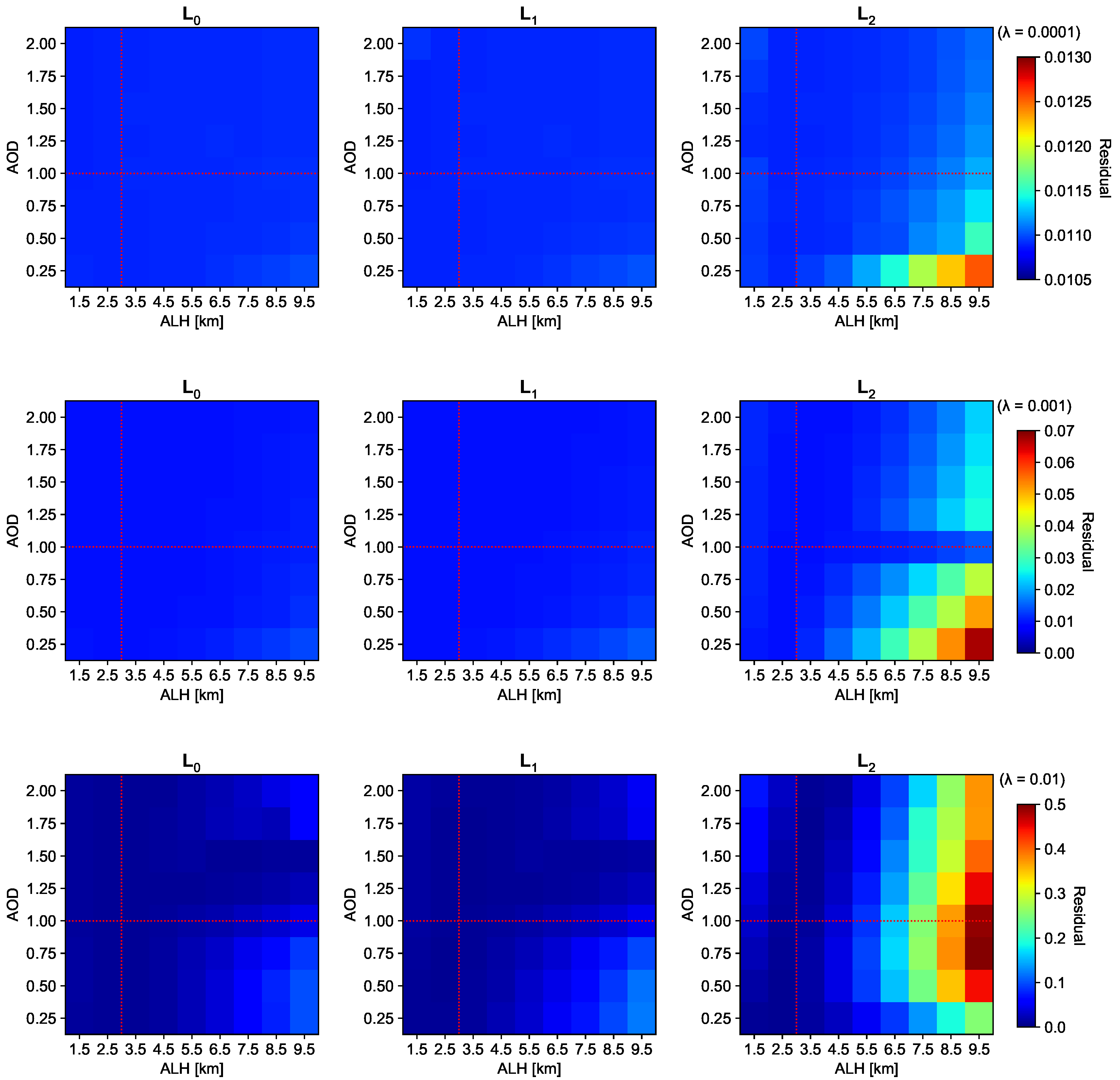
3.2. Aerosol Retrieval

A satellite hyperspectral spectrometer called TROPOspheric Monitoring Instrument (TROPOMI) was developed to measure global distributions of trace gases, aerosols, and clouds. The instrument comprised four spectrometer modules that covers the UV-VIS (270–495 nm) and NIR (675–775 nm), and the shortwave IR spectral range (2305–2385 nm). The O₂A-band (758–770 nm) was particularly designed to derive the height information of aerosols and clouds. Here, we carried out an experiment of aerosol properties retrieval from synthetic TROPOMI O₂A-measurements. The relevant setup of aerosol microphysical properties and geometry/surface conditions is given in

Table 4. The parameterization of aerosol model, geometry, and surface for generating synthetic TROPOMI O₂A-measurements.

Parameter	Description
Aerosol model	“moderately absorbing” [49,50]
Surface albedo	0.06
Solar zenith angle	30${}^{\circ }$
Viewing zenith angle	0${}^{\circ }$
Relative azimuth angle	180${}^{\circ }$

. The synthetic TROPOMI data were generated with a set of aerosol properties, i.e., the aerosol layer height (ALH) and optical depth (AOD).

The forward model $F$ is described in Section 2.1.1. In contrast to the profile retrieval in Section 3.1, the state vector $x$ in this case had two components, i.e., ALH and AOD. In this case, the Jacobian matrix $\mathbf{K}\left(x\right)$ depicts the contribution of the aerosol properties to the radiance, i.e., $\mathbf{K}\left(x\right)=\partial F/\partial x$, with $x=[X_{\mathrm{ALH}},X_{\mathrm{AOD}}]$. The components of $x$ in this section were different from those for the temperature profile retrieval in Section 3.1. Thus, ${\mathbf{L}}_C$ calculated from the a priori profile covariance matrix was not available for comparison. The initial guess $x_0$ and a priori $x_{\mathrm{a}}$ were assumed to be identical with 3 km and 1 corresponding to ALH and AOD, respectively. The inverse problem in the aerosol retrieval was considered to be mildly/moderately ill-posed as the order of magnitude of the condition number was about 2. A suitable form of the penalty term ($\mathbf{L}$) was expected to be influential as compared to a cautiously-chosen regularization strength ($\lambda$). In this experiment, the classical TR with three values of $\lambda$ (0.0001, 0.001, and 0.01) was employed. A better retrieval performance with a smaller $\lambda$ would be anticipated.

The errors of ALH retrieval using the three regularization matrices are shown in Figure 3 in terms of the relative difference to the true value. In this figure and the following ones, the ($x,y$) coordinates represent the pairs of true values of ALH and AOD. The best retrieval result was obtained with the lowest $\lambda$ and the relative error was essentially within 5%. The retrieval results using ${\mathbf{L}}_0$ and ${\mathbf{L}}_1$ were reasonable and the error became larger in the case of the measurements with lower AODs. Both were significantly better than that of ${\mathbf{L}}_2$ with the larger $\lambda$. Underestimations were frequently found in the retrievals using all three forms of $\mathbf{L}$ when $\lambda =0.01$, except for the measurements with lower ALHs. The retrieval error reached up to −60% from the measurements with larger ALHs. Besides the too strong regularization, this was caused by unreliable a priori information.

The relative errors of AOD retrieval are displayed in Figure 4. Similar to the ALH retrieval, the retrieval performance of ${\mathbf{L}}_0$ and ${\mathbf{L}}_1$ was comparable and better than that of ${\mathbf{L}}_2$. Nevertheless, the difference of the AOD retrieval between the three forms of $\mathbf{L}$ was not recognizable compared to that of the ALH retrieval. When $\lambda =0.0001$, the retrieval error of ${\mathbf{L}}_0$ and ${\mathbf{L}}_1$ was within 3% and smaller than that of ${\mathbf{L}}_2$ (∼5%); when $\lambda =0.01$, an error of up to 20% could be seen in the case using ${\mathbf{L}}_2$. The retrieved AODs were particularly overestimated from the measurements with lower AODs and higher ALHs. These results indicated a possible correlation between the retrieved AOD and ALH. In the case of higher ALHs, a negative correlation between ALH and AOD was noticed and turned out to be stronger for ${\mathbf{L}}_2$. For smaller values of $\lambda$, this correlation became weaker.

According to the retrieval output in Figure 3 and Figure 4, the retrieved quantities using ${\mathbf{L}}_0$ and ${\mathbf{L}}_1$ approximated the true state in most cases. The retrieval trended to be worse using larger values of $\lambda$ as the a priori error was also notable. Regarding the ALH retrieval, the retrieval using ${\mathbf{L}}_1$ was slightly better than that using ${\mathbf{L}}_0$, whereas ${\mathbf{L}}_0$ marginally outperformed ${\mathbf{L}}_1$ in the case of the AOD retrieval. The retrieval using ${\mathbf{L}}_2$ achieved the acceptable accuracy with $\lambda =0.0001$ but could produce the larger error with a factor of 2–3 with an inappropriate $\lambda$.

In addition to the retrieved aerosol parameters, Figure 5 depicts the corresponding residual after convergence. Unsurprisingly, for all the forms of $\mathbf{L}$, the residual decreased while the $\lambda$ decreased. As the ALH increased, the residual corresponding to ${\mathbf{L}}_2$ considerably increased, whereas only a gradual increase was found in the residuals corresponding to the other two matrices. This increasing trend between the residual and AOD did not seem to be linear, especially in the case of lower AODs. In other words, the spectrum in the spectral range of interest seemed to be more influenced by the contribution of ALH. The residuals corresponding to ${\mathbf{L}}_0$ and ${\mathbf{L}}_1$ were comparable and apparently better than that corresponding to ${\mathbf{L}}_2$.

In contrast to the temperature retrieval in Section 3.1, the aerosol retrieval dealt with two independent properties. The retrieval performance of ${\mathbf{L}}_0$ was greatly improved as it managed to approximate the true magnitude of the solution. The retrieval using ${\mathbf{L}}_1$ also produced satisfactory results even when the a priori state was far from the true state. However, the retrieval performance of ${\mathbf{L}}_2$ was not convincing in the case that suboptimal choice of $\lambda$ was used.

4. Conclusions

The penalty term of the Tikhonov-type objective function plays an important role in solving atmospheric retrieval problems. The goal of this paper was to give an insight into the impact of the regularization matrix. The design of this matrix can crucially affect the retrieval performance and greatly degrade the inversion accuracy.

We have performed retrievals of atmospheric temperature profile and aerosol properties using the identity matrix ${\mathbf{L}}_0$, discrete approximations of the first and second order derivative operators ${\mathbf{L}}_1$ and ${\mathbf{L}}_2$, respectively. For the temperature profile retrieval, the Cholesky factor of the a priori profile covariance matrix ${\mathbf{L}}_{\mathrm{C}}$ has also been included. The pros and cons of each regularization form have been analyzed.

The temperature retrieval from an airborne microwave radiometer demonstrates that the inversion algorithms enable reliable retrieval only within a limited altitude range. This is mainly because of the measurement characteristics. Although reliable a priori information appears to be important, the retrieval performance of ${\mathbf{L}}_1$ and ${\mathbf{L}}_2$ is superior to that of ${\mathbf{L}}_0$ and ${\mathbf{L}}_{\mathrm{C}}$ in case of large a priori errors.

The aerosol properties retrieval from a satellite hyperspectral spectrometer shows that the performance of ${\mathbf{L}}_0$ and ${\mathbf{L}}_1$ is evidently better than that of ${\mathbf{L}}_2$. The retrieval errors are within 5% while imposing weak regularization strength.

Based on the numerical experiments, we may draw the following conclusions:

• ${\mathbf{L}}_0$ has a good control on the magnitude of the solution;
• ${\mathbf{L}}_1$ imposes the smoothness of the solution with satisfactory retrieval accuracy even when the a priori information is not reliable;
• ${\mathbf{L}}_2$ also tends to produce a smoothed solution, but the retrieval accuracy can be degraded when the a priori information is not reliable;
• ${\mathbf{L}}_{\mathrm{C}}$ associates with the a priori information.

Although the observation geometry and spectral range are drastically different, ${\mathbf{L}}_1$ turns out to be favorable due to its “robustness” in both experiments. Nevertheless, a definite choice for the universal form of $\mathbf{L}$ may not exist, as the best one could always be problem dependent. From a practical point of view, the application of ${\mathbf{L}}_1$ (and sometimes ${\mathbf{L}}_2$) is beneficial when the desired solution (e.g., profile retrieval) is expected to be smooth. ${\mathbf{L}}_0$ is a preferable choice when the desired solution prefers the magnitude.

References

1. Engl, H.; Hanke, M.; Neubauer, A. Regularization of Inverse Problems; Kluwer Academic Publishers: Dordrecht, The Netherlands, 2000. [Google Scholar]
2. Kress, R. Linear Integral Equations, 3rd ed.; Applied Mathematical Sciences; Springer: New York, NY, USA, 2014. [Google Scholar] [CrossRef]
3. Twomey, S. Introduction to the Mathematics of Inversion in Remote Sensing and Indirect Measurements; Elsevier Science: Amsterdam, The Netherlands, 1977. [Google Scholar]
4. Stephens, G. Remote Sensing of the Lower Atmosphere; Oxford University Press: Oxford, UK, 1994. [Google Scholar]
5. Rodgers, C. Inverse Methods for Atmospheric Sounding: Theory and Practise; World Scientific: Singapore, 2000. [Google Scholar]
6. Efremenko, D.; Doicu, A.; Loyola, D.; Trautmann, T. Acceleration techniques for the discrete ordinate method. J. Quant. Spectrosc. Radiat. Transf. 2013, 114, 73–81. [Google Scholar] [CrossRef]
7. del Águila, A.; Efremenko, D.S.; Molina García, V.; Xu, J. Analysis of two dimensionality reduction techniques for fast simulation of the spectral radiances in the Hartley-Huggins band. Atmosphere 2019, 10, 142. [Google Scholar] [CrossRef] [Green Version]
8. del Águila, A.; Efremenko, D.S.; Thomas, T. A review of dimensionality reduction techniques for processing hyper-spectral optical signal. Light Eng. 2019, 27, 85–98. [Google Scholar] [CrossRef] [Green Version]
9. Hansen, P. Rank-Deficient and Discrete Ill-Posed Problems: Numerical Aspects of Linear Inversion; SIAM: Philadelphia, PA, USA, 1998. [Google Scholar]
10. Vogel, C. Computational Methods for Inverse Problems; SIAM: Philadelphia, PA, USA, 2002. [Google Scholar]
11. Doicu, A.; Trautmann, T.; Schreier, F. Numerical Regularization for Atmospheric Inverse Problems; Springer: Berlin/Heidelberg, Germany, 2010. [Google Scholar] [CrossRef] [Green Version]
12. Hansen, P. Discrete Inverse Problems: Insight and Algorithms; SIAM: Philadelphia, PA, USA, 2010. [Google Scholar] [CrossRef]
13. Tikhonov, A. On the Solution of Incorrectly Stated Problems and a Method of Regularization. Dokl. Acad. Nauk SSSR 1963, 151, 501–504. [Google Scholar]
14. Tikhonov, A.; Arsenin, V. Solutions of Ill-Posed Problems; Wiley: Hoboken, NJ, USA, 1977. [Google Scholar]
15. Allmaras, M.; Bangerth, W.; Linhart, J.; Polanco, J.; Wang, F.; Wang, K.; Webster, J.; Zedler, S. Estimating Parameters in Physical Models through Bayesian Inversion: A Complete Example. SIAM Rev. 2013, 55, 149–167. [Google Scholar] [CrossRef] [Green Version]
16. Eriksson, P. Analysis and comparison of two linear regularization methods for passive atmospheric observation. J. Geophys. Res. 2000, 105, 18157–18167. [Google Scholar] [CrossRef]
17. Brezinski, C.; Rodriguez, G.; Seatzu, S. Error estimates for linear systems with applications to regularization. Numer. Algorithms 2008, 49, 85–104. [Google Scholar] [CrossRef]
18. Xu, J.; Schreier, F.; Doicu, A.; Trautmann, T. Assessment of Tikhonov-type regularization methods for solving atmospheric inverse problems. J. Quant. Spectrosc. Radiat. Transf. 2016, 184, 274–286. [Google Scholar] [CrossRef] [Green Version]
19. Ceccherini, S. Analytical determination of the regularization parameter in the retrieval of atmospheric vertical profiles. Opt. Lett. 2005, 30, 2554–2556. [Google Scholar] [CrossRef]
20. Ridolfi, M.; Sgheri, L. A self-adapting and altitude-dependent regularization method for atmospheric profile retrievals. Atmos. Chem. Phys. 2009, 9, 1883–1897. [Google Scholar] [CrossRef] [Green Version]
21. Koner, P.K.; Drummond, J.R. A comparison of regularization techniques for atmospheric trace gases retrievals. J. Quant. Spectrosc. Radiat. Transf. 2008, 109, 514–526. [Google Scholar] [CrossRef]
22. Thomas, G.; Stamnes, K. Radiative Transfer in the Atmosphere and Ocean; Cambridge University Press: Cambridge, UK, 1999. [Google Scholar] [CrossRef]
23. Liou, K.N. An Introduction to Atmospheric Radiation, 2nd ed.; Academic Press: Cambridge, MA, USA, 2002. [Google Scholar]
24. Bohren, C.F.; Clothiaux, E.E. Fundamentals of Atmospheric Radiation; Wiley-VCH Verlag: Weinheim, Germany, 2006. [Google Scholar]
25. Petty, G.W. A First Course in Atmospheric Radiation, 2nd ed.; Sundog Publishing: Madison, WI, USA, 2006. [Google Scholar]
26. Zdunkowski, W.; Trautmann, T.; Bott, A. Radiation in the Atmosphere — A Course in Theoretical Meteorology; Cambridge University Press: Cambridge, UK, 2007. [Google Scholar]
27. Dahlback, A.; Stamnes, K. A new spherical model for computing the radiation field available for photolysis and heating at twilight. Planet. Space Sci. 1991, 39, 671–683. [Google Scholar] [CrossRef]
28. Wick, G. über ebene Diffusionsprobleme. Z. Phys. 1943, 121, 702–718. [Google Scholar] [CrossRef]
29. Chandrasekhar, S. Radiative Transfer; Dover Publications Inc.: New York, NY, USA, 1960. [Google Scholar]
30. Stamnes, K.; Tsay, S.C.; Wiscombe, W.; Jayaweera, K. Numerically Stable Algorithm for Discrete–Ordinate– Method Radiative Transfer in Multiple Scattering and Emitting Layered Media. Appl. Opt. 1988, 27, 2502–2509. [Google Scholar] [CrossRef] [PubMed]
31. Efremenko, D.S.; Molina García, V.; Gimeno García, S.; Doicu, A. A review of the matrix-exponential formalism in radiative transfer. J. Quant. Spectrosc. Radiat. Transf. 2017, 196, 17–45. [Google Scholar] [CrossRef] [Green Version]
32. Schreier, F.; Gimeno García, S.; Hedelt, P.; Hess, M.; Mendrok, J.; Vasquez, M.; Xu, J. GARLIC—A general purpose atmospheric radiative transfer line-by-line infrared-microwave code: Implementation and evaluation. J. Quant. Spectrosc. Radiat. Transf. 2014, 137, 29–50. [Google Scholar] [CrossRef] [Green Version]
33. Schreier, F.; Gimeno García, S.; Hochstaffl, P.; Städt, S. Py4CAtS—PYthon for Computational ATmospheric Spectroscopy. Atmosphere 2019, 10, 262. [Google Scholar] [CrossRef] [Green Version]
34. Dennis, J., Jr.; Schnabel, R.B. Numerical Methods for Unconstrained Optimization and Nonlinear Equations; SIAM: Philadelphia, PA, USA, 1996. [Google Scholar] [CrossRef]
35. Eriksson, P.; Jiménez, C.; Buehler, S.A. Qpack, a general tool for instrument simulation and retrieval work. J. Quant. Spectrosc. Radiat. Transf. 2005, 91, 47–64. [Google Scholar] [CrossRef] [Green Version]
36. Wehr, T.; Bühler, S.; von Engeln, A.; Künzi, K.; Langen, J. Retrieval of stratospheric temperatures from spaceborne microwave limb sounding measurement. J. Geophys. Res. Atmos. 1998, 103, 25997–26006. [Google Scholar] [CrossRef]
37. von Engeln, A.; Bühler, S. Temperature profile determination from microwave oxygen emissions in limb sounding geometry. J. Geophys. Res. Atmos. 2002, 107, ACL-12. [Google Scholar] [CrossRef]
38. Stähli, O.; Murk, A.; Kämpfer, N.; Mätzler, C.; Eriksson, P. Microwave radiometer to retrieve temperature profiles from the surface to the stratopause. Atmos. Meas. Tech. 2013, 6, 2477–2494. [Google Scholar] [CrossRef] [Green Version]
39. Massaro, G.; Stiperski, I.; Pospichal, B.; Rotach, M.W. Accuracy of retrieving temperature and humidity profiles by ground-based microwave radiometry in truly complex terrain. Atmos. Meas. Tech. 2015, 8, 3355–3367. [Google Scholar] [CrossRef] [Green Version]
40. Denning, R.F.; Guidero, S.L.; Parks, G.S.; Gary, B.L. Instrument description of the airborne microwave temperature profiler. J. Geophys. Res. Atmos. 1989, 94, 16757–16765. [Google Scholar] [CrossRef]
41. Mahoney, M.; Denning, R. A State-of-the-Art Airborne Microwave Temperature Profiler (MTP). In Proceedings of the 33rd International Symposium on the Remote Sensing of the Environment, Stresa, Italy, 4–8 May 2009. [Google Scholar]
42. Gary, B.L. Mesoscale temperature fluctuations in the stratosphere. Atmos. Chem. Phys. 2006, 6, 4577–4589. [Google Scholar] [CrossRef] [Green Version]
43. Nielsen-Gammon, J.W.; Powell, C.L.; Mahoney, M.; Angevine, W.M.; Senff, C.; White, A.; Berkowitz, C.; Doran, C.; Knupp, K. Multisensor estimation of mixing heights over a coastal city. J. Appl. Meteorol. Climatol. 2008, 47, 27–43. [Google Scholar] [CrossRef]
44. Davis, C.A.; Ahijevych, D.A.; Haggerty, J.A.; Mahoney, M.J. Observations of Temperature in the Upper Troposphere and Lower Stratosphere of Tropical Weather Disturbances. J. Atmos. Sci. 2014, 71, 1593–1608. [Google Scholar] [CrossRef]
45. Voigt, C.; Schumann, U.; Minikin, A.; Abdelmonem, A.; Afchine, A.; Borrmann, S.; Boettcher, M.; Buchholz, B.; Bugliaro, L.; Costa, A.; et al. ML-CIRRUS: The airborne experiment on natural Cirrus and contrail cirrus with the High-Altitude Long-Range Research Aircraft HALO. Bull. Am. Met. Soc. 2017, 98, 271–288. [Google Scholar] [CrossRef]
46. Kenntner, M.; Fix, A.; Jirousek, M.; Schreier, F.; Xu, J.; Rapp, M. Measurement Characteristics of an airborne Microwave Temperature Profiler (MTP). Atmos. Meas. Tech. Discuss. 2020, 2020, 1–55. [Google Scholar] [CrossRef] [Green Version]
47. Gordon, I.; Rothman, L.; Hill, C.; Kochanov, R.; Tan, Y.; Bernath, P.; Birk, M.; Boudon, V.; Campargue, A.; Chance, K.; et al. The HITRAN2016 molecular spectroscopic database. J. Quant. Spectrosc. Radiat. Transf. 2017, 203, 3–69. [Google Scholar] [CrossRef]
48. Anderson, G.; Clough, S.; Kneizys, F.; Chetwynd, J.; Shettle, E. AFGL Atmospheric Constituent Profiles (0–120 km); Technical Report TR-86-0110; AFGL: Hanscom, MA, USA, 1986. [Google Scholar]
49. Levy, R.C.; Remer, L.A.; Mattoo, S.; Vermote, E.F.; Kaufman, Y.J. Second-generation operational algorithm: Retrieval of aerosol properties over land from inversion of Moderate Resolution Imaging Spectroradiometer spectral reflectance. J. Geophys. Res. Atmos. 2007, 112. [Google Scholar] [CrossRef] [Green Version]
50. Levy, R.C.; Remer, L.A.; Dubovik, O. Global aerosol optical properties and application to Moderate Resolution Imaging Spectroradiometer aerosol retrieval over land. J. Geophys. Res. Atmos. 2007, 112. [Google Scholar] [CrossRef] [Green Version]
Figure 1. Comparison of temperature retrievals for case 1. The initial guess and true profile are blue and green lines, respectively. Retrieved temperature profiles (left panel) and the corresponding differences to the true profiles (right panel) are shown for the four regularization matrices.
Atmosphere 11 01052 g001
Figure 2. Comparison of temperature retrievals for case 2. Retrieved temperature profiles are shown for the four regularization matrices. The left and right panels correspond to two scenarios using different true profiles.
Atmosphere 11 01052 g002
Figure 3. Error of aerosol layer height (ALH) retrieval for three regularization matrices. The x- and y-axes represent the true values of ALH and aerosol optical depth (AOD), respectively. The value of λ is displayed above each color bar. The dotted red lines refer to the a priori values of ALH and AOD.
Atmosphere 11 01052 g003
Figure 4. Error of AOD retrieval for three regularization matrices. The x- and y-axes represent the true values of ALH and AOD, respectively. The value of λ is displayed above each color bar. The dotted red lines refer to the a priori values of ALH and AOD.
Atmosphere 11 01052 g004
Figure 5. Residual after convergence corresponding to three regularization matrices. The x- and y-axes represent the true values of ALH and AOD, respectively. The values of λ is displayed above each color bar. The dotted red lines refer to the a priori values of ALH and AOD.
Atmosphere 11 01052 g005