Review

How Can Odors Be Measured? An Overview of Methods and Their Applications

Politecnico di Milano, Department of Chemistry, Materials and Chemical Engineering “Giulio Natta”-P.za Leonardo da Vinci 32, 20133 Milano, Italy
*
Author to whom correspondence should be addressed.
Atmosphere 2020, 11(1), 92; https://doi.org/10.3390/atmos11010092
Submission received: 19 December 2019 / Revised: 4 January 2020 / Accepted: 8 January 2020 / Published: 13 January 2020

Abstract

:
In recent years, citizens’ attention towards air quality and pollution has increased significantly, and nowadays, odor pollution related to different industrial activities is recognized as a well-known environmental issue. For this reason, odors are subjected to control and regulation in many countries, and specific methods for odor measurement have been developed and standardized over the years. This paper, conceived within the H2020 D-NOSES project, summarizes odor measurement techniques, highlighting their applicability, advantages, and limits, with the aim of providing experienced as well as non-experienced users a useful tool that can be consulted in the management of specific odor problems for evaluating and identifying the most suitable approach. The paper also presents relevant examples of the application of the different methods discussed, thereby mainly referring to scientific articles published over the last 10 years.

1. Introduction

In recent years, citizens’ attention towards air quality and pollution has increased significantly, and nowadays, odor pollution related to different industrial activities, such as agricultural activities, chemical industries, waste treatment and disposal facilities, and oil and gas extraction or refining facilities, is recognized as a well-known environmental issue [1].
Although odor emissions are generally considered harmless, in some cases, they cause citizens to complain to local authorities [2]. Indeed, populations do not generally perceive several conventional pollutants, even if the exposure limit concentrations are exceeded. On the contrary, odors can be perceived far below normal exposure limit concentrations, because some odorous compounds have extremely low odor detection threshold concentrations [3].
For this reason, odors are nowadays subjected to control and regulations in many countries, and specific methods for odor measurement have been developed [3,4]. As will be discussed in the next paragraphs, such methods include both sensorial and instrumental techniques, with each having specific advantages and drawbacks. The most important methods for odor measurement include:
  • Dynamic olfactometry;
  • Chemical analysis (with speciation or non-specific);
  • Gas chromatography-olfactometry (GC-O);
  • Tracer analysis;
  • Instrumental odor monitoring by e-noses;
  • Field inspection;
  • Field olfactometry; and
  • Citizen science.
Dynamic olfactometry and field inspection are the only methods specifically developed for odor measurement, which have been standardized at the European level [5,6,7].
Other techniques, involving chemical characterization, are consolidated analytical techniques, commonly adopted to provide information about the odor properties of gaseous mixtures.
Conversely, methods based on citizen science are quite new. Those techniques, based on the active involvement of citizens, have been proposed in recent years to address socio-environmental conflicts within the impacted communities [8,9]. In particular, these programs consist of the active involvement of citizens in the mapping and management of odor pollution problems, thereby allowing co-creation of local solutions together with industries, regional and local authorities, and odor experts [10,11]. With the aim to develop such innovative approaches based on so-called “extreme citizen science”, in 2018, the Distributed Network for Odor Sensing, Empowerment, and Sustainability (D-NOSES) project was presented and has received funding from the European’s Union Horizon 2020 Science with and for Society Call (SwafS) under grant agreement No. 789315. This project proposes a holistic approach, based on the cooperation of key stakeholders (citizens, regional and local authorities, industries, and odor experts) for the mapping and co-design of solutions, to researching, building, and suggesting an appropriate regulatory framework. Recognizing the lack of information about odor pollution and management as a limit for the successful adoption of citizen science for the management of odor problems, this review paper was conceived within the H2020 D-NOSES project with the purpose of raising awareness about odor pollution and providing a scientific background concerning odor impact assessment methods, which can be used by experienced as well as non-experienced users.
This paper presents an overview of the methods that can be used for odor measurement, thereby excluding odor impact assessment techniques based on mathematical methods (i.e., dispersion models) or literature evaluations.
Indeed, dispersion models have become increasingly popular for odor impact assessment purposes over the last 20 years [12,13,14,15], and most European regulations on odor impacts are based on modelling approaches [16,17]. The decision to exclude odor dispersion models from the present overview is because there is already extensive literature on the matter [18,19,20], and because the specific goal of this review paper was to provide an exhaustive answer to the question: “How can odors be measured?”
Section 2 is structured in subsections relevant to the different methods, providing a brief description of each technique and some examples of the relevant applications by referring to the scientific literature prevailingly over the last 10 years (a few older works have also been cited if particularly relevant). These examples do not have the aim of representing an exhaustive review of all the literary studies regarding the specific measurement method, but a limited set of scientific studies have been selected to point out the specific applicability and limitations of each method.
Finally, the last section proposes a comparison of the different approaches in terms of their applicability and limitations, with the purpose of providing a useful tool that can be consulted for the evaluation and identification of the most suitable methods for any specific odor pollution problem.

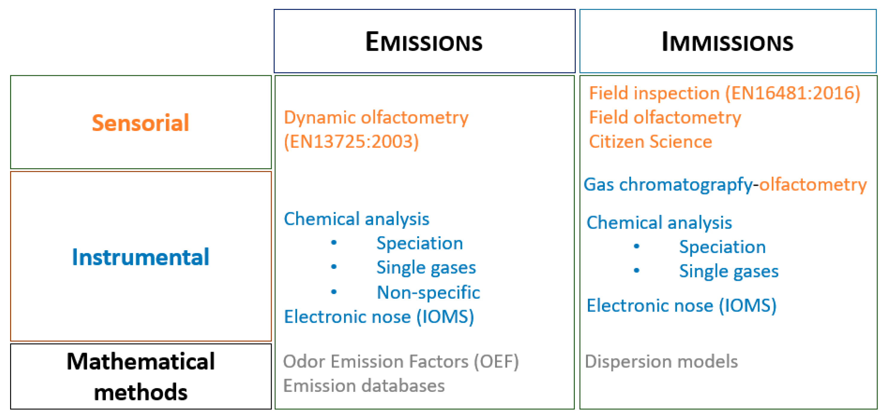
2. Overview of Odor Impact Assessment Methods

2.1. General Schematization of Odor Impact Assessment Methods

Over the years, diverse methods have been studied and developed for the characterization of environmental odors, with the purpose of assessing the odor impact of industrial activities on surrounding territories. A first step for this work was identifying the existing methods for odor impact assessment and trying to schematize them in a rather simple way depending on the type of approach and its applicability.
Thus, Figure 1 proposes a schematization based on the type of approach (mathematical methods, instrumental measurements, and sensorial measurements) and where the methods can be applied, i.e.,
  • Emissions: For measuring odors at emission sources; and
  • Receptors: For measuring odors in ambient air, directly where citizens are located and where complaints come from.
As already mentioned, among all the methods for odor impact assessment, this overview only focuses on the methods for odor measurements, leaving out mathematical methods.

2.2. Dynamic Olfactometry

2.2.1. Brief Description of the Method

Dynamic olfactometry is a sensorial method standardized by the European Standard EN 13725:2003 [5], which provides the odor concentration of a sample, referring to the sensation that it causes in a panel of opportunely selected people directly exposed to that odor.
The odor concentration, expressed in European odor units per cubic meter (ouE/m3), represents the number of dilutions with neutral air that are necessary to bring the concentration of the sample to its odor detection threshold (OT), i.e., the threshold at which the odor is perceived by 50% of the examiners. To put it in the simplest manner, if the sample needs to be diluted 100 times with clean air so that the panel cannot perceive the odor anymore, this means that the sample has a concentration of 100 ouE/m3.
The analysis is carried out by presenting the sample to the examiners (i.e., panelists) at increasing concentrations by means of a dilution device, called an olfactometer, which dilutes the samples according to given ratios with reference air, which is made odor- and humidity-free through filtration with active carbon or silica gel.
In order to ensure reliable and repeatable results, the EN 13725:2003 fixes precise criteria for panel selection based on individuals’ threshold for n-butanol in nitrogen (between 20 and 80 ppb) and the standard deviation of the individual’s responses, which should be verified periodically.

2.2.2. Applicability and Limitations

Dynamic olfactometry is used to characterize odor emission sources. Indeed, in providing objective information about odor concentration, it can be used alone to assess the efficiency of odor abatement systems or in combination with dispersion models to evaluate odor impacts caused by different odor-emitting activities on the surrounding communities.
The combination of the odor concentration with the information related to the emitted airflow, geometry, and nature of the emission source allows the evaluation of the odor emission rate (OER), which is basically the odor flux emitted to the atmosphere, and is the parameter that effectively accounts for the amount of odor that is emitted into the atmosphere by a given source.
The OER is expressed in ouE/s and is obtained as the product of the odor concentration by the air flow associated with the source. The method adopted for estimating OER depends on the source type, i.e., point, volume, or surface sources [21].
This datum can be used as input data for specific mathematical models, which combine this information together with meteorological and geographical data, and thus calculate how the emitted odor is transported through the atmosphere to the affected citizens. Over the last few years, there has been significant research investigating how to adequately estimate OER values from different source types, which are commonly considered as “complex” [22,23,24,25,26].
On the other hand, dynamic olfactometry has the disadvantage of being a discontinuous measurement method, since samples are collected at the source in a precise moment and then transported and analyzed in a laboratory. For this reason, it cannot be used to continuously monitor odor emissions. Moreover, dynamic olfactometry provides only a quantitative characterization of odors and cannot be used to identify odors or distinguish between different odors.

2.2.3. Examples of Applications

The objective determination of odor concentration provided by dynamic olfactometry makes this odor measurement method a useful tool for the assessment of the overall performance and efficiency of abatement systems in removing odors and volatile organic compounds (VOCs).
Recent examples of the adoption of this technique to test the efficiency of industrial biofilters by means of the characterization of samples collected upstream and downstream from the abatement units was discussed by Gutierrez et al. in 2015 [21] and Sowka et al. in 2017 [27], proving the applicability of dynamic olfactometry as a tool for performance verification. Moreover, this type of characterization allowed verification of the compliance of the odor concentrations measured at investigated emissions with regulatory limits fixed by the competent authorities.
Gutierrez et al. [21] also proposed the combination of dynamic olfactometry with gas chromatography-time of flight/mass spectrometry GC-TOF/MS (which will be discussed in the next paragraph), with the aim of identifying, among the VOCs analyzed, the compounds responsible for the odor emission.
The most common application of dynamic olfactometry entails its combination with dispersion modelling, since determining only the odor concentration in emissions is not sufficient to assess the odor impact on citizens.
In 2010, Sironi et al. [28] presented a case study regarding the assessment of the odor impact in the presence of multiple similar sources, i.e., four rendering plants. Based on the results of olfactometric surveys carried out in different seasons, the authors estimated the overall odor emission rates emitted by each plant and identified the major contributor to the odor impact on the monitored area. The results of this investigation were used as input for the CALPUFF model, the outcome of which allowed quantification of the odor impact relevant to the four monitored plants on the surroundings.
In 2019, Romanik et al. [29] presented a comparative analysis, based on the combination of dynamic olfactometry and dispersion modelling, of the emission scenario relevant to an industrial activity before and after the installation of abatement equipment. The results obtained satisfied the twofold purpose of the study of proposing an experimental procedure to assess the odor impact at the sensible receptors and to evaluate the effectiveness of the technical intervention in the reduction of odorous emissions.

2.3. Chemical Analysis with Speciation

2.3.1. Brief Description of the Method

Chemical analysis (with speciation) of odors is an instrumental method for odor characterization that involves the complete identification and quantification of chemical compounds in an odor sample.
The most common technique proposed in the scientific literature is gas chromatography coupled with mass spectrometry (GC-MS) (Figure 2).
GC-MS combines the separation capability of gas chromatography (GC), based on the chemical-physical properties of the mixture constituents, with mass spectrometry (MS), which, breaking each molecule into ionized fragments, provides a unique fingerprint (mass spectrum) of the compounds detected, thereby allowing identification of the mixture constituents.

2.3.2. Applicability and Limitations

At the emission level, GC-MS can be applied in order to obtain information about the chemical composition of odor emissions. Indeed, the identification and quantification of the chemical compounds that are present in odor emissions are fundamental to evaluate the impact of emitted compounds on the environment and human health.
Chemical characterization also allows evaluation of the compliance of emissions with regulatory concentrations or flux limits that are fixed by the competent authorities in order to protect workers and citizens from exposure to hazardous or toxic compounds.
One way to relate the chemical composition of an odorous mixture to its odor concentration is to evaluate the so called odor activity value (OAV). The OAV is defined as the sum of the ratio between the chemical concentration of each compound in the mixture and its odor threshold (OT) concentration:
O A V = i = 1 n C i O T i ,
where OAV = odor activity value (ouE m−3); Ci = concentration of the compound i (mg m−3); and OTi = odor threshold of the compound i (mg ouE−1).
However, although GC-MS was historically the first method applied for odor characterization, chemical analysis may not always be effective in the characterization of complex odors. Indeed, this approach allows adequate estimation of the odor concentration only in the case of odorous samples containing few chemicals. Anyhow, since real samples (e.g., composting exhaust gases, emissions from wastewater treatments plants) are usually complex mixtures, their odors can hardly be related to their chemical composition, and odor concentrations calculated through OAV can be very imprecise [30].
One reason for this imprecision is the difficulty of finding reliable OT values, given that the values that are found in the literature for a single odorous compound often differ by several orders of magnitude [31,32]. Moreover, synergic or masking effects between chemicals may occur, resulting in odors completely unrelated to the chemical composition [33]. As a consequence, this approach might provide misleading results.
Finally, often, VOCs, which are responsible for the odor properties of gaseous mixtures, are present at concentrations in the range of ppb or even ppt, which is lower than the instrumental detection limit. Therefore, pre-concentration techniques are commonly adopted before GC-MS. Common pre-concentration techniques include adsorption of the static headspace on active carbons followed by thermal desorption (TD), purge and trapping, and solid phase microextraction (SPME) [34,35].

2.3.3. Examples of Applications

Although chemical analysis does not provide information directly related to odor perception, several scientific papers have proposed this technique for the characterization of odorous emissions and for the assessment of the odor impact [36,37,38].
Many researchers have applied chemical analysis with speciation to characterize odors from waste treatment and composting plants, with the aim of identifying the compounds that are most frequently responsible for odor emissions, as well as the most suitable treatment methods to limit them. In 2011, Font et al. [39] summarized in a review paper the analytical (chemical) methods used to detect and quantify compounds constituting emissions from the composting and anaerobic digestion facilities of waste, together with the treatment methods applied to gaseous emissions that are commonly used in this type of plant. The application examples reported in [40] indicated that correlations between the odor concentration estimated by OAV and dynamic olfactometry can hardly be established, although specific compounds responsible for the odor of the mixture have been identified. For example, Mao et al. [40] determined ammonia, amines, dimethyl sulfide, and acetic acid as being responsible for most odors in food waste-composting plants compared to numerous VOCs, but no correlation between the chemical analyses and odor concentrations was reported. D’Imporzano et al. [41] pointed out that as the biological stability increases during the entire anaerobic digestion process, the odor emissions measured by olfactometry decrease, although no correlation between total VOCs and olfactometry could be established.
In 2013, Murphy et al. [42] proposed thermal desorption-gas chromatography/mass spectrometry (TD-GC/MS) for the characterization of non-methane volatile organic compounds (NMVOCs) emitted from mechanically ventilated poultry sheds in similar stages of broiler production. The authors developed an experimental protocol for the chemical characterization of odorous samples and multivariate calibration models to study the relationship between NOMVOCs and odor in five broiler sheds. The results obtained proved the applicability of chemical analysis for the identification of ubiquitous odor predictors for the samples under investigation and allowed an assessment of the relationships between ubiquitous odor predictors and other measured NMVOCs that also contribute to the odor properties of emissions from sheds.
In 2017, Wu et al. [43] proposed the adoption of gas chromatography to assess the odor impact of a landfill in Beijing (China). Odorous samples collected seasonally were analyzed by both chemical analysis and an olfactometer to correlate the measured odor concentration with the calculated odor concentration by means of the odor activity value (OAV). With an awareness of the variability of odor thresholds (OTs) reported in the scientific literature, the authors measured the OT using the forced-choice ascending concentration series method and sniffing panelists, with the aim of minimizing the imprecision of the estimated odor concentration. This approach allowed a relatively higher correlation coefficient (r = 0.9194) to be obtained between the measured and estimated odor concentrations. The speciation of odor samples collected at the main landfill odor sources led to the identification of compounds mostly responsible for the odors under investigation, i.e., hydrogen sulfide, dimethyl sulfide, and trimethylamine.
GC-MS is also commonly adopted for monitoring emission variations during industrial processes to identify the most critical phases, which significantly influence the odor’s impact on the surroundings. In 2019, Gonzalez et al. [44] used TD GC-MS to characterize odorous emissions of a full-scale sewage composting plant located in Majorca (Spain). In particular, the study involved the analysis of 34 gaseous samples representative of different points of the treatment processes, with the aim of monitoring the odorous emissions during the composting process. The results pointed out that the odorous emissions tended to decrease as the biological stability of the material increased and allowed identification of the compounds that were most responsible for the emission of odor. The authors evaluated the possibility of defining a correlation between the odor concentrations estimated by means of OAVs and those assessed by field olfactometry. However, a weak correlation was found between the OAVs and odor concentration values, pointing out the abovementioned criticalities concerning the quantification of odors by means of OAV estimation due to OT variability and the neglect of synergic or masking effects between odorants.
Chemical analysis with speciation can be used also to monitor the efficiency of abatement systems. As an example, in 2015, Gutierrez et al. [21] used GC-TOF/MS in conjunction with dynamic olfactometry to monitor the performance of an industrial-scale biofilter. The speciation of chemical compounds allowed the identification of the compounds that were most responsible for odor emissions, even at very low concentrations (i.e., ppt). The identification of groups of families that have similar influences on the variance of the measure resulted in minimization of the number of compounds tested during frequent performance checks of the biofilter, while also reducing the cost and analysis time.
Recently, chemical analysis has also been proposed for the characterization of odors at the receptor level. In 2017, Bylinsky et al. [45] investigated the capability of two-dimensional gas chromatography coupled with a time of flight mass spectrometer and field olfactometry for the characterization of odor properties of atmospheric air in Gdansk, where a wastewater treatment plant (WWTP) and an oil refinery are located. The study involved the analysis of five samples collected by means of absorption tubes in ambient air around the oil refinery and WWTP. This investigation allowed identification of the main pollutant present in the atmosphere in the area adjacent to the industrial activities. However, the results obtained could not be directly related to the odor emissions under examination, because they might be influenced by the background. The authors pointed out that similar ranges for odor concentrations estimated from the chemical composition and measured by dynamic olfactometry were obtained, but no specific correlation was reported in the paper.

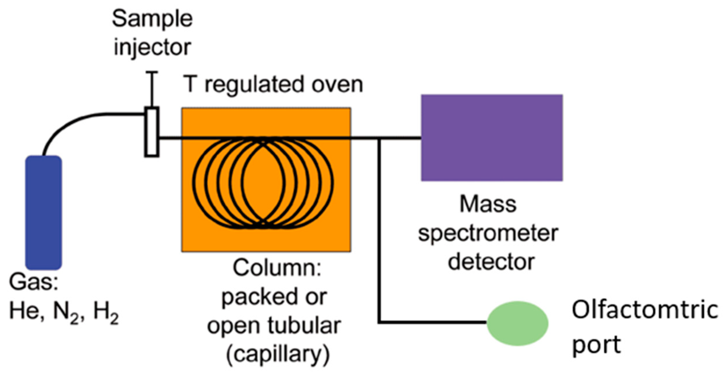
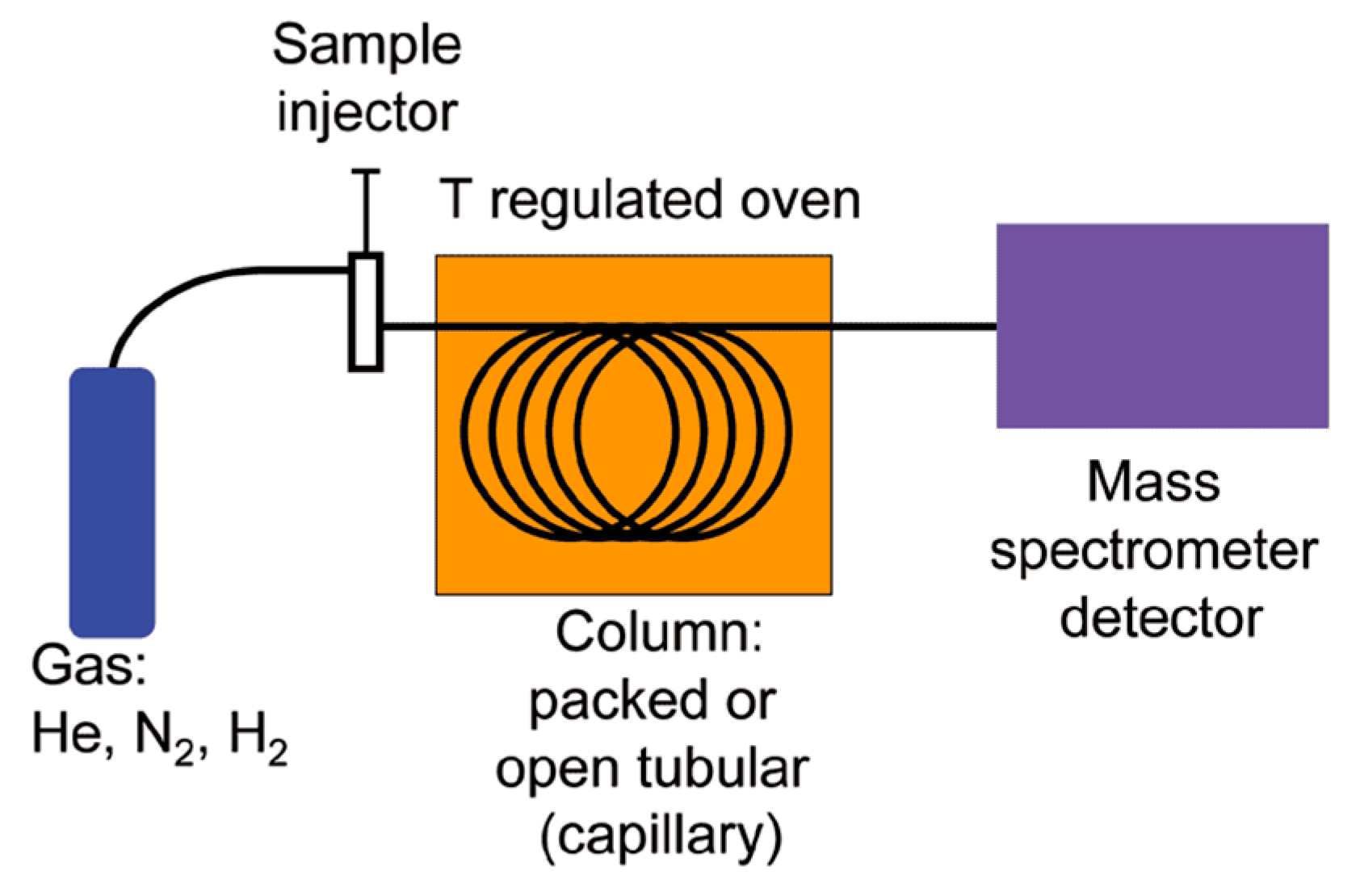
2.4. Gas Chromatography-Olfactometry GC-O

2.4.1. Brief Description of the Method

Gas chromatography analysis with olfactometric detection (GC-O) couples traditional gas chromatography analysis with human olfaction to detect volatile organic compounds eluting from GC separation (Figure 3) [46]. In particular, GC-O involves a gas chromatography-mass spectrometry (GC-MS) system equipped with an olfactory detection port: At the end of the GC column, the eluted flux is divided into equal portions between the MS detector and the olfactory port. The trained panelist sniffs the gas at the olfactory port and provides a sensorial response in terms of the odor presence, odor quality, and odor intensity [47]. Various GC-O techniques have been developed to determine the relative importance of odorants in a sample. They can be classified into three categories [47]:
  • Detection frequency:
    The same sample is analyzed by a panel of assessors (6–12 panelists) in order to provide the percentage of people who detect the odor compound at a given retention time. Each odor can be evaluated using the nasal impact frequency (NIF) or surface of nasal impact frequency (SNIF) values. The NIF is set at one when each of the evaluators senses a given odor and zero when no one senses any odor at a given retention time. The NIF value corresponds to the peak height of the olfactometric signal while the SNIF value represents the peak areas obtained by multiplying the frequency percentage by the duration.
  • Dilution to threshold:
    Dilution to threshold methods provide a quantitative description of the odor potential of a given compound based on the ratio between its concentration in the sample and its sensory threshold in air. These methods involve the preparation of a dilution series of samples, using two-fold, three-fold, five-fold, or 10-fold dilution levels and analyzing them by GC-O. The panelist indicates under which dilution the compound can still be sensed and describes the type of smell. The most common dilution methods are aroma extract dilution analysis (AEDA) and combined hedonic aroma response measurement (CharmAnalyisTM). AEDA measures the highest sample dilution at which the odor is still detectable (flavor dilution factor, FD). CharmAnalyisTM records the duration of odors and generates chromatographic peaks.
  • Direct intensity:
    Direct intensity methods measure the intensity and duration of odors using different types of quantitative scales: Category scales or unstructured scales. These methods include a single time-averaged measurement registered after the elution of the analyte, or a dynamic measurement, where the appearance of the odor, its maximum intensity, and the decline are recorded continuously (OSME). In the first case, the panelist assigns a value from a previously defined scale to each detected compound while in the second case, an olfactogram, which similar to conventional chromatograms, is obtained, in which the peak corresponds to the maximum intensity and width of the odor duration.

2.4.2. Applicability and Limitations

GC-O, whose applicability is limited to emissions, provides information about the odor character associated with different constituents of the odorous mixture, which allows estimation of the relative influence of single components on the total odor of the sample. In general, it is used in cases of real mixtures constituted by odorous compounds characterized by strong odors and low odor thresholds.
However, GC-O is a cost- and time-intensive method, which does not allow estimation of the odor concentration of samples, because odors present in different concentrations, all above the detection threshold, will produce aromagrams with peaks of the same intensity. Moreover, since it operates on the separation of the sample into its single components, the olfactory properties of the sample as a whole are not considered. For this reason, data from GC-O analysis cannot provide information about the odor impact, and can neither be used directly as input for dispersion modelling.

2.4.3. Examples of Applications

Common applications of GC-O involve the characterization of emissions aimed at qualitatively and quantitatively analyzing the key odorant mainly responsible for the olfactory properties of emission sources.
As an example, in 2010, Zhang et al. [48] focused on the development of an odor characterization method for quantitative analysis of the key odorants responsible for livestock odor by means of thermal desorption coupled with multidimensional gas chromatography-mass spectrometry-olfactometry (TD-MDGC-MS/O). The target compounds were separated in the GC column and the isolated compounds were split into the mass detector and sniff port in order to assess their concentration and olfactory properties (odor character, intensity, duration time, and hedonic tone). In 2015, the authors extended the study of 15 typical VOCs associated with livestock odor, identified the most significant gases that contribute to the relative odor impacts of livestock buildings, and estimated a correlation between the odor intensity and chemical concentration [49].
In 2018, Fisher et al. [37] proposed the adoption of gas chromatography/olfactometry to characterize odor emissions from wastewater treatment plants, proving the potentialities of GC-O for the identification of compounds responsible for emission odors throughout biosolid processing, and a description of their odor properties was provided by odor wheels.

2.5. Chemical Analysis—Non-Specific

2.5.1. Brief Description of the Method

Non-specific chemical characterization can be used as a screening tool in those cases in which the odor problem is specifically related to hydrocarbon molecules.
Non-specific chemical analysis involves the use of easily transportable and quite cheap tools, like FID (flame ionization detector) or PID (photo ionization detector) detectors, as screening tools to assess the total amount of hydrocarbons.
Both FID and PID detectors pyrolyze the organic compounds present in the analyzed gas and provide the concentration of all ionizable chemicals present in the sample. The main difference between the two instruments is the ionization mechanism.
The flame ionization detector (FID) (Figure 4) is a burner in which a regulated flow of the gas sample passes through a flame sustained by regulated flows of a fuel gas (a hydrogen/diluent mixture) and air. Within the flame, the hydrocarbon components of the sample stream undergo a complex ionization that produces electrons and positive ions. In order to detect these ions, two electrodes are used to provide a potential difference [50].
The photo ionization detector (PID) uses ultraviolet light to irradiate the sample, thus ionizing it. The analysis chamber is composed of two plates between which a difference of potential is applied. Upon the production of ionized molecules, a current is created and recorded (Figure 5). The intensity of the current is a direct measure of the number of ionized molecules [51].
The main difference between these two kinds of sensors is that the FID needs a hydrogen bottle to maintain a hydrogen flame as an energy source while the PID uses a UV lamp. Because of this different ionization mechanism, a FID is also able to detect methane, which is odorless, while a PID, which has a weaker energy source, is useful for detecting NMHCs (non-methanic hydrocarbons).
The output of these types of instruments is the total VOC concentration expressed in terms of the concentration equivalent to the calibration gas concentration.

2.5.2. Applicability and Limitations

Non-specific chemical analysis is very useful for the detection of gas leaks, which represent potential odor emissions, for example, hydrocarbon fugitive emissions from equipment or piping in refineries or landfill gas leaks from covers.
The main drawback of this method is that it does not provide any information about the odor properties of the analyzed gas. The total hydrocarbon concentration that is measured cannot be directly related to the odor concentration. Indeed, in the scientific literature, it is known that the correlation between the total VOC concentration and the odor concentration of gas samples is generally hard to estimate or nonexistent [19]. Moreover, these instruments do not take into consideration the different odor thresholds of different compounds, the response factors of the electric sensor, and the mixing effects.

2.5.3. Examples of Applications

Non-specific chemical analysis is commonly adopted to estimate fugitive emissions.
Many authors have proposed different techniques in the scientific literature for the detection and quantification of gas leaks. As an example, in 2008, Chambers et al. [52] proposed the adoption of differential absorption light detection and ranging (DIAL) to remotely measure the concentration profiles of hydrocarbons from the equipment and piping of a refinery. Their approach allowed measurement of the concentration profiles in the atmosphere up to several hundred meters away. When combined with the wind speed and direction, downwind vertical DIAL scans can be used to calculate mass fluxes of the measured gas leaving the site. This rapid estimation of fugitive leaks would improve the effectiveness of efforts to reduce emissions, quantify the reduction in emissions, and improve the accuracy of emissions data that are reported to regulators and the public.
Similar characterization approaches were also proposed in the scientific literature for the estimation of landfill fugitive emissions. In 2010, Fredenslund et al. [53] developed a method for the quantification of gas emissions from the leachate collection system at landfills, based on FID measurements. They presented the emission data measured at two Danish landfills with no landfill gas collection systems in place: Fakse landfill and AV Miljø. The emission rates observed from individual leachate collection wells at the two landfills ranged from 0.1 to 76 kgCH4d−1. The results of the quantification of fugitive emissions, when continuously measuring emissions from a leachate well over a week, highlighted the strong influence on emission rates caused by the rise and fall in atmospheric pressure.
In 2011, Di Bella et al. [54] evaluated CH4 diffuse emissions, based on direct measurements carried out with the flux accumulation chamber (static, non-stationary) method, and also obtained a CH4 contoured flux map of the landfill. Such emissions were compared with the estimate achieved by means of CH4 mass balance equations. The results showed that the emissions obtained by applying the flux chamber method were in good agreement with the ones derived by the application of the mass balance equation, and that the evaluated contoured flux maps represent a reliable tool to locate areas with abnormal emissions in order to optimize the efficiency of gas recovery systems.
In 2018, Kormi et al. [55] proposed the adoption of the genetic algorithm-based optimization combined with standard Gaussian dispersion model to estimate fugitive landfill methane emissions by identifying locations and emissions rates. The authors presented the results of four case studies, carried out to evaluate the performance of the proposed methodology, which proved its applicability and effectiveness in the estimation of landfill methane emissions. Despite being an interesting demonstration of this type of analysis coupled with dispersion modelling, it should, however, be highlighted that methane emissions are not necessarily correlated with odor emissions.

2.6. Chemical Analysis—Single Gases

2.6.1. Brief Description of the Method

In those rare cases in which the odor pollution problem is due mainly to the presence of a single compound (tracer), a reliable quantification of odors can be obtained by assessing the concentration of those single gases. In environmental odor monitoring, ammonia and hydrogen sulfide are often monitored as common tracers for odorous emissions.
Depending on the concentration ranges expected, different tools can be adopted for the odorous target compound quantification.
When the concentrations are quite high (1–10 ppm), electrochemical sensors, which are easy to use and cheap, can be adopted. Electrochemical sensors couple a chemically selective layer to an electrochemical transducer. This way, the chemical energy of the selective interaction between the sensor and the target compound is transduced into an analytical signal, which can be correlated to the concentration of the target compound. Those sensors are grouped according to the electrical magnitude used for transduction in potentiometric, conductimetric, impedimetric, and amperometric titration [56].
When concentrations are in the range of ppb, more complex and expensive tools for target compounds’ quantification, like a chemiluminescence analyzer for NH3 or gold leaf analyzers for H2S, are needed.
The chemiluminescence analyzer for NH3 converts NH3 into NO and utilizes chemiluminescence technology for a reaction that produces a characteristic luminescence with an intensity proportional to the amount of NO. Those tools are highly reliable and are characterized by their long-term stability.
Gold leaf analyzers are frequently used to monitor hydrogen sulfide traces in the gas phase. They measure the H2S concentration by monitoring the change in the resistance of a gold film sensor caused by the adsorption of H2S molecules [57]. A common gold leaf analyzer is the Jerome 631-X H2S analyzer.

2.6.2. Applicability and Limitations

Chemical analysis targeting the detection of single gases can be applied both to emissions or in ambient air. For emissions, it can be useful to verify compliance to emission limits relevant to specific compounds. When applying the analysis of single gases to ambient air, the compound to be measured should not be ubiquitous and its source must be clearly identifiable.
This approach has the main advantage of being simple and relatively cheap. Moreover, in cases in which the emitted odor is directly correlated to one specific compound (tracer), the measured tracer concentration can be used to estimate the odor concentration emitted. In such cases, this datum can be used as input for dispersion modelling to evaluate the odor’s impact on communities. For this purpose, it is necessary to preliminarily assess a correlation between the compound concentration and the odor concentration [58].
On the contrary, the chemical characterization of single gases is useless in the case of complex odorous mixtures, whereby the odor concentration is not related to the concentration of one single component, but it is a mixture of hundreds of different compounds. In those cases, it may be combined with other techniques for a more comprehensive odor characterization [58,59,60].

2.6.3. Examples of Applications

In the scientific literature, examples of applications at both the emissions and receptor level have been reported and in many cases, the chemical characterization of tracers is combined with other odor impact assessment methods.
In 2007, Qu et al. [61] proposed the use of an integrated system, including an electronic nose, an H2S detector, and an NH3 detector, to predict the odor concentration at emission sources. In particular, the study involved the analysis of odorous samples from swine manure sources. Both linear regression and artificial neural networks were applied to develop correlations. Single detectors proved to be capable of predicting the odor concentration with poor accuracy (i.e., about 50%), whereas the integrated system achieved a good performance (R2 = 0.75).
In 2018, Cangialosi et al. [59] presented a case study involving the installation of a Jerome H2S analyzer for the continuous monitoring of odor emissions at a landfill boundary. The H2S analyzer was integrated with an automatic air sampler, which was activated in the case of an alert of the H2S detector to withdraw samples to be sent for olfactometric analysis. The results pointed out that no correlation was found between the continuous H2S measurements by the Jerome J605 analyzer and the ouE/m3 values obtained by dynamic olfactometry.
In 2011, Heaney et al. [62] investigated the relationship between malodor, ambient hydrogen sulfide, health, and quality of life in a community bordering a landfill. Landfill neighbors were enrolled and kept twice-daily diaries for 14 days about odor intensity, alteration of daily activities, mood states, and irritant and other physical symptoms. Concurrently, hydrogen sulfide air measurements were recorded every 15 min. Relationships between H2S, odor, and health outcomes were evaluated using conditional fixed effects regression models. The results highlighted that landfill odor increased 0.63 points (on a 5-point Likert-type scale) for every 1 ppb increase in hourly average H2S when the wind was blowing from the landfill towards the community and that odor was strongly associated with reports of alterations of daily activities or healthy symptoms.
In 2012, Blanes-Vidal et al. [63] investigated the association between the regional and temporal variation of ammonia concentration in five Danish non-urban regions and environmental odor annoyance perceived by local residents. NH3 concentration was obtained from air pollution monitoring stations. This study provided evidence that the NH3 concentration measured and modeled as part of national air quality programs could be used as a proxy of the prevalence of odor annoyance in non-urban residential communities.

2.7. Instrumental Odor Monitoring (E-Noses)

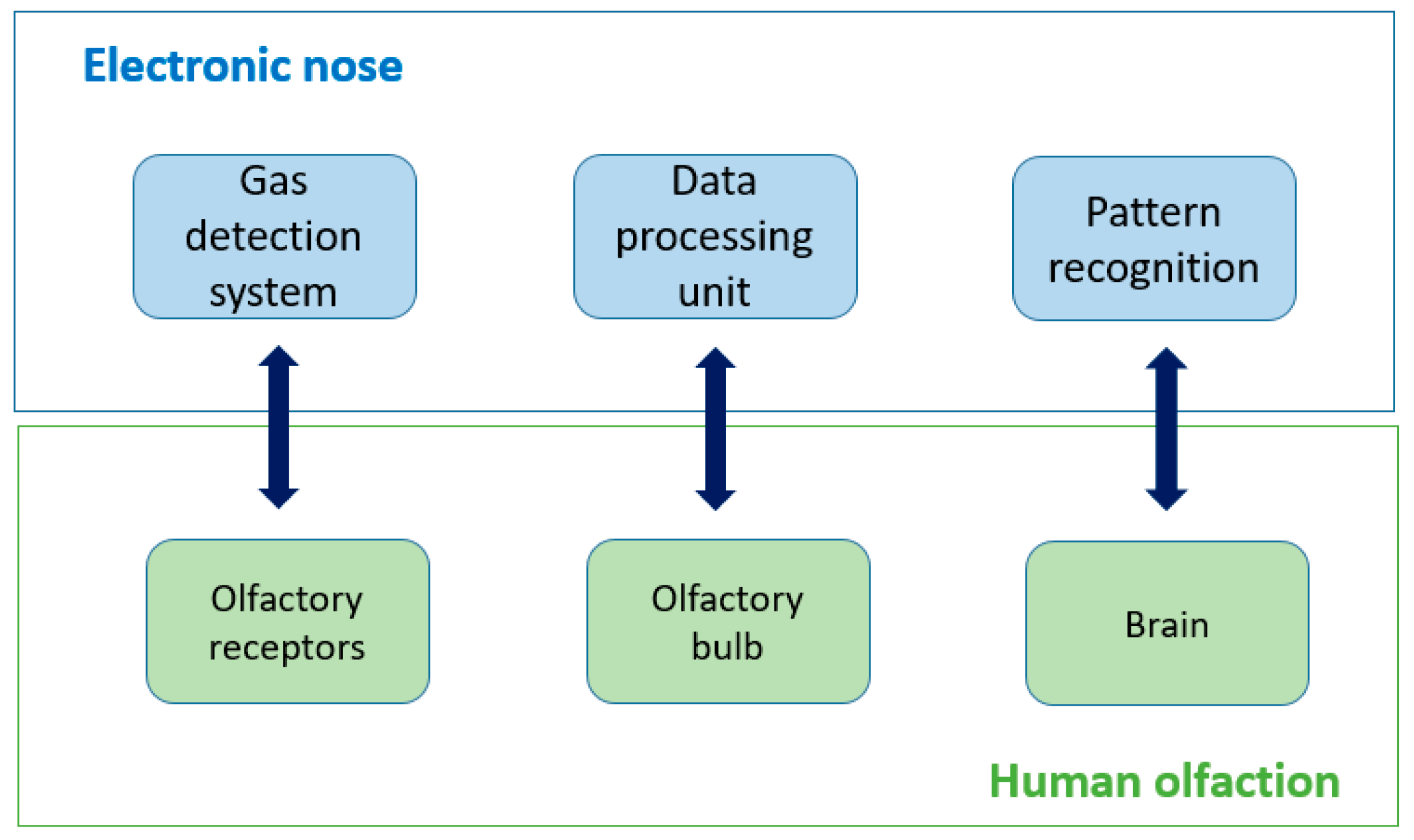
2.7.1. Brief Description of the Method

Electronic noses are instruments designed to mimic mammalian olfaction in the detection and characterization of simple or complex odors. These devices allow the characterization of mixtures of organic samples as a whole, providing their olfactory fingerprint, without recognizing the individual odor-generating compounds, as the human nose does [64,65].
To do this, the instrument must be trained: It must be provided with a database of olfactory fingerprints relating to the odors to which it may be exposed to during the analysis. That database is put together by analyzing gaseous samples with known olfactory qualities at different odor concentrations, thus defining the olfactory classes (odor types) to be recognized.
The e-nose architecture can be divided into the following three components (Figure 6) [65]:
  • Gas detection system: This is an array of n gaseous sensors, which may differ in type and operational temperature, housed into a chemically inert box, which respond to the presence of VOCs with variations of their chemical-physical properties [66,67]. The gas detection system mimics the function of human olfactory receptors.
  • Data processing unit: This system, as the human olfactory bulb, compresses the transient responses of the sensors, eliminates signal noise, and extracts features relevant for pattern recognition.
  • Classification or pattern recognition: A classification algorithm identifies odors based on a dataset that must have been previously stored. In particular, when presented with an unidentified sample, the classification assigns to it a class label by comparing its fingerprint with those compiled during the training.
During operation, the air is continuously pulled by a vacuum pump through a tube into the chemically inert box, where the sensor array is housed. The interaction of VOCs with the sensors’ active material produces a transient response, which reaches a steady state condition in a few minutes. During this interval (i.e., response time of the sensor array), the sensor responses are recorded and delivered to the signal-processing unit.
The data processing procedure, through which the electronic nose identifies an odorant sample, can be described as a sequence of the following three sequential stages [68]:
  • Signal pre-processing and feature extraction;
  • Dimensionality reduction; and
  • Classification or clustering.
Signal pre-processing compensates for sensor drift and compresses transient sensor responses by means of manipulation of the sensor baselines or normalization of the sensors’ response ranges for all the sensors in an array [68].
Feature extraction has the purpose of extracting the information relevant for pattern recognition from the sensor array response while the dimensionality reduction stage projects the n-dimensions of the multidimensional dataset onto a few informative and independent axes to simplify data inspection and avoid problems related to redundancy [63]. The resulting low-dimensional projection can be more readily inspected visually: Measurements are points of the discarded plot. Feature extraction can be performed with different common techniques for multivariate statistical analysis, such as principal component analysis (PCA), linear discriminant analysis (LDA), or Sammon nonlinear maps.
Once the measurements have been projected, the classifier produces an estimate of the class for an unknown sample along with an estimate of the confidence placed on the class assignment, comparing its odor fingerprint with those previously compiled in the training phase. Many algorithms for the classification task based on different statistical methods have been developed during the years. In general, the k-nearest neighbors (k-NNs), support vector machine (SVM), random forest (RF), and artificial neural networks (ANNs) are most commonly adopted [67,69,70,71].

2.7.2. Applicability and Limitations

Electronic noses can be used both at emissions and receptors for the continuous characterization of odors [72].
In the case of emissions, an e-nose can be used to continuously monitor the efficiency of odor abatement systems. Although e-noses cannot completely substitute dynamic olfactometry in the assessment of odor concentrations because instrument training requires that the odor concentration of samples must be known, trained e-noses can provide an estimation of the odor concentrations of unknown samples, if a specific correlation between the sensor responses and dynamic olfactometry results has been assessed in the training phase [60,69]. Recent advances in pattern recognition techniques (including partial least square-discriminant analysis, artificial neural networks, Kohonen self-organizing maps, principal component analysis, and vector machine classifiers) have allowed for enhanced identification of unknown samples, with correlations in the range 80–95% to odor concentrations measured using olfactometry [38]. Therefore, specifically trained e-noses can be installed at the outlet of abatement systems to continuously monitor odor emissions, thereby providing real-time information about the function of the equipment and allowing rapid intervention in case of failures. Moreover, data collected at emission sources by e-noses can be used as input data for dispersion modelling [73,74,75].
In the case of receptor-level applications, the e-nose continuously characterizes ambient air in terms of the odor’s presence and quality in order to provide a direct assessment of the odor impact of industrial activities at the receptor. This type of analysis, in the case of multiple sources, allows identification of the sources that are most responsible for the perception of odors at receptors through the recognition of odor provenance. Electronic noses are widely used for environmental odor monitoring, since they can create continuous and fast results with a limited budget.
However, e-noses cannot provide information about the intensity and hedonic tone (pleasantness) of the odor.

2.7.3. Examples of Applications

Electronic noses can be used to monitor industrial processes. For example, in 2002, Figueiredo and Stentiford [76] used an e-nose to monitor the composting process and detect the transition from aerobic to anaerobic conditions, using a laboratory reactor with a controlled temperature.
In 2012, Delgado-Rodriguez et al. [77] evaluated the use of an electronic nose as on-line, rapid method to quantify the gases from municipal solid waste (MSW) composting. The electronic nose detected a clear difference in the volatile compounds profiles relevant to the gases emitted during composting, using principal component analysis (PCA). PCA reduced the dataset resulting from the sensor responses to two principal components, which accounted for 74.5%, 68.8%, and 62.8% of the total variance by using patterns of the initial, thermophilic, and mesophilic composting phases, respectively.
E-noses can also be used to continuously monitor industrial emissions. In 2018, Cangialosi et al. [59] investigated the possibility of using a multisensory electronic nose and an H2S continuous analyzer to continuously monitor the malodors from a sanitary landfill for non-hazardous waste, located in Southern Italy. The electronic nose was trained towards landfill odors and after installation, it proved its effectiveness for on-line monitoring, quantification, and identification of the odor produced by the landfill. On the contrary, detection by the continuous H2S analysis was poorly correlated with the odor concentration in ambient air measured by dynamic olfactometry.
The most common application of an electronic nose in the environmental field concerns the assessment of the odor impact directly where the odor presence is lamented.
In 2007, Sironi et al. [78] presented the monitoring of odors from a composting plant by two electronic noses, which were installed in a nearby house and inside the perimeter of the composting plant to compare the responses of both instruments. The instruments were trained with samples collected at the odor sources. Samples were characterized by dynamic olfactometry and, depending on their odor concentration, diluted with odorless air, with the aim of providing the instruments with odor concentrations to which they might be exposed to during the monitoring. The odor impact was assessed in terms of the frequency of landfill odor detection by the electronic nose over the monitoring period. The results of the study proved the effectiveness of the e-nose as a cheap tool for direct assessment of the odor impact at receptors.
In 2017, Deshmukh et al. [79] investigated the real-time measurement of municipal solid waste odors using both an electronic nose and chemical analyzers, with the aim of developing mathematical models to predict the odor concentration. The samples collected at major odor sources over a period of 50 days were processed by principal component analysis (PCA) to build the classification model and by Monte Carlo simulation and multilinear regression (MLR) to build the correlation for estimating the odor concentration.
In 2018, Licen et al. [80] presented e-nose monitoring of an integrated cycle steel plant in Trieste (Italy) and discussed the building of a classification model by means of a chemometric approach based on self-organizing maps (SOMs). The study involved an e-nose equipped with 4 metal oxide semiconductor (MOS) and 15 polymer/black carbon composite sensors and chemical nitrogen and sulfur sensors, which were trained considering ambient air samples collected after citizens’ calls and olfactometric characterization. To assess the recall ability of the map, a small number of e-nose signals registered in correspondence with other olfactometric measurements were used. The method proposed proved that the SOM map was able to classify malodor events coherently. Moreover, the odor control map provides valuable visualization support in following the dynamic evolution of the system over time.
In 2018, Orzi et al. [81] proposed the adoption of electronic noses for the assessment of the odor impact of untreated cow and pig slurries and treated (digestate and liquid fraction of digestate) manures when they were used on soil at the field scale. The study involved an analysis by means of dynamic olfactometry and a portable electronic nose PEN3, equipped with 10 MOS sensors, of samples collected by means of a flux chamber both under lab conditions and in the field. The study proposed the comparison of results relevant to different conditions of sampling, with the aim of investigating the effect of anaerobic digestion on odor emissions. The results obtained highlighted that anaerobic digestion stabilizes slurries and reduces the variability among different matrices, independent of their origin, and proved the applicability of e-nose technology as an emission-monitoring tool.
In a recent publication of 2019 [82], we discussed the application of two very different electronic nose instruments for the monitoring of odor emissions from a landfill located in Northern Italy. Besides describing the methodology adopted in order to determine the landfill odor impact, the paper described the field tests carried out in order to assess the instrument performances and compared them according to a specified procedure. This aspect is particularly interesting for the purpose of e-noses’ qualification, which is one of the main critical issues related to the development of specific standards for the diffusion of such instruments as air quality-monitoring tools [83].

2.8. Field Inspection

2.8.1. Brief Description of the Method

Field inspection provides the characterization of odor exposure in a defined assessment area. It involves the use of qualified panel members in the field to directly assess the presence of recognizable odors linkable to a specific source in ambient air.
Two different approaches for field inspection can be applied:
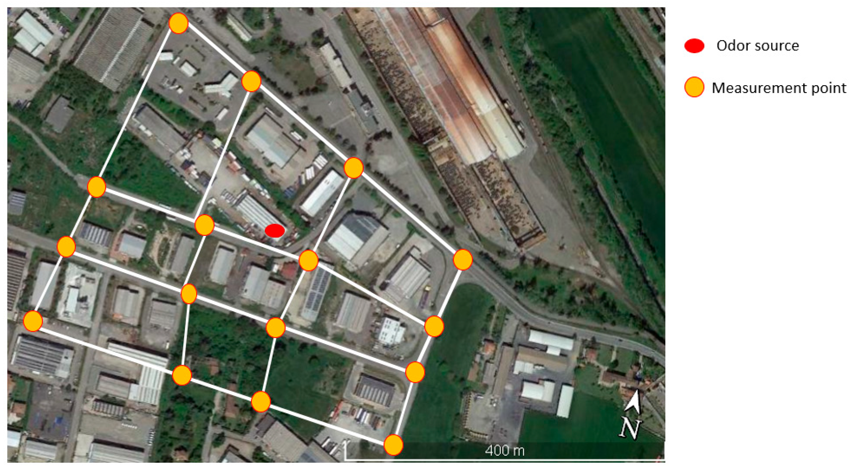
  • Grid method (EN 16841-1:2016) [6]: This uses direct assessment of ambient air by panel members to characterize odor exposure in a defined assessment area; and
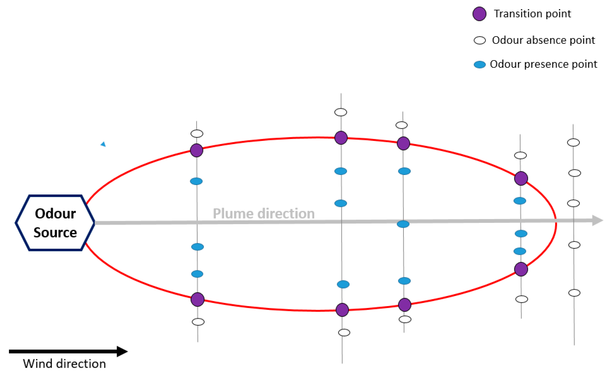
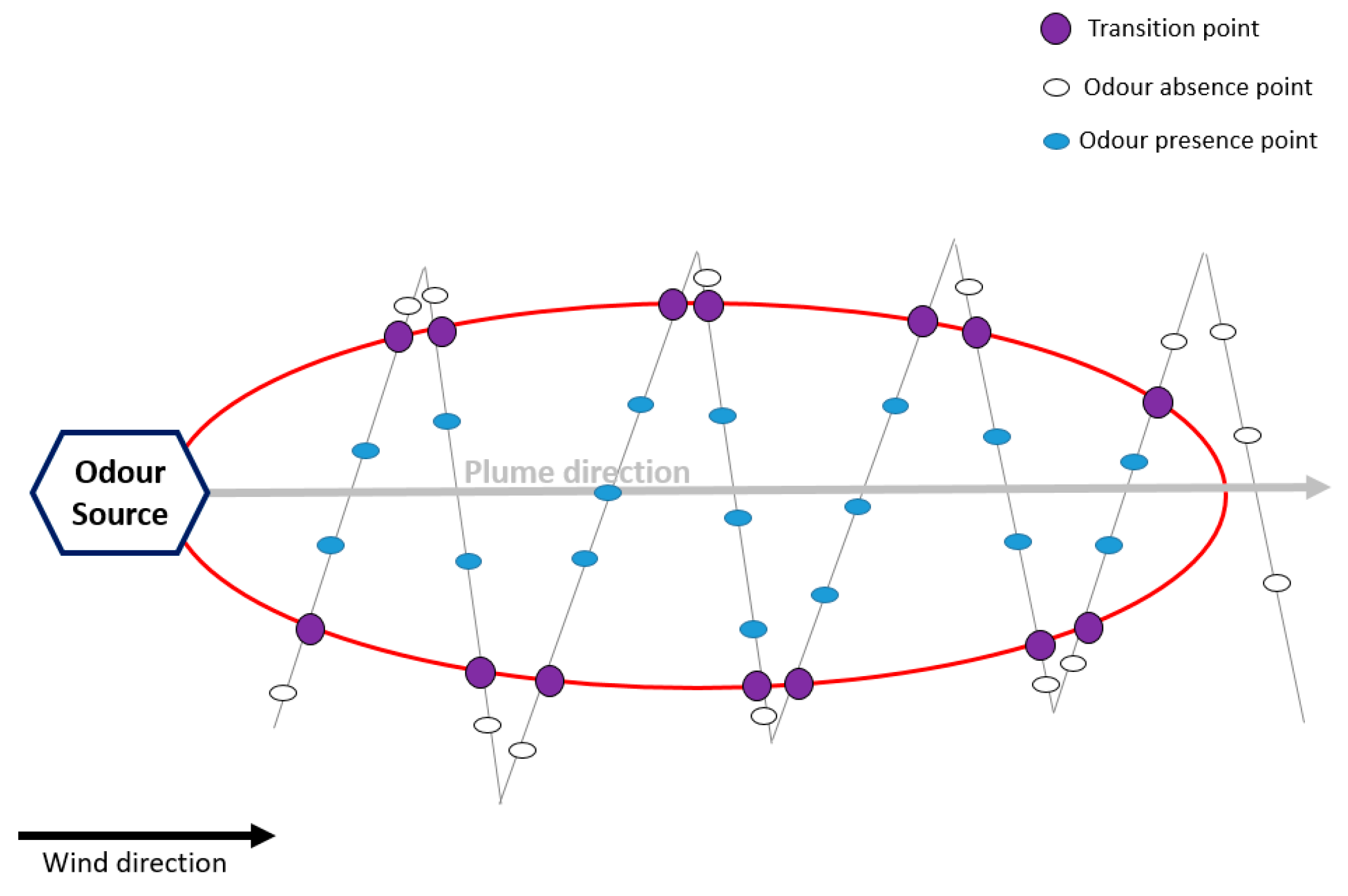
  • Plume method (EN 16841-2:2016) [7]: This determines the extent of the downwind odor plume of a defined source under specific meteorological conditions.
The grid method [6] is a statistical survey method that is applied on an assessment area over a sufficiently long period of time that can be representative of the weather conditions in the area to provide a representative map of the odor exposure.
The unit of measurement of the method is the frequency of odor hours for a square of evaluation, defined by four measurement points, as a representative value for exposure to odors. For each point of the grid, repeated measurements must be carried out during the monitoring time frame, so that the evaluation can be representative of all the phases of activity of the characterized source.
During the analysis, the panel inhales the ambient air for 10 min and records a classification every 10 s. Each observation gives indications about the presence/absence of odor and, in the case of recognition, of the type of odor. By summing up the total number of single measurements conducted at these four measurement points, the odor hour frequency is calculated.
If a particular odor type exceeds a percentage odor time of 10% (i.e., the presence of odor is detected in six or more out of 60 observations), the result is classified as an odor hour.
Figure 7 reports an example of an assessment area in the surroundings of an odor emission source with assessment squares and measurement points.
The plume method [7] is used to determine the extent of the area where the odor plume originating from a specific odor source can be perceived and recognized under specific meteorological and operating conditions. The extent of the odor plume is described by points where a transition from the absence to presence of the recognizable odor under investigation occurs.
The analyses of ambient air are carried out by panel members at different points downwind to the source under well-defined meteorological conditions.
The stationary plume method or dynamic plume method can be used as observation methods.
Using the stationary plume method (Figure 8), the panel members are located at specific intervals along intersection lines perpendicular to the plume direction. Many panel members are located at intervals along each intersection line to cover the estimated width of the recognizable plume and carry out the analysis simultaneously. Each member determines the percentage of odor time in the course of one single measurement. If the result of a single measurement the percentage is lower than 10%, the odor is considered as being absent; otherwise, the odor is present.
Using the dynamic plume method (Figure 9), the panel members cross the plume while conducting single measurements at frequent intervals by successively entering and exiting the plume at different distances from the emission source, including distances where no recognizable odors is detected. In this way, they determine the transition between the absence and presence of recognizable odors and the extent of the plume. The maximum plume reach estimate is defined as the distance along the plume direction between the source and the point halfway from the furthest crossing where the odor presence is recorded.
For both approaches, the plume extent is defined by transition points., i.e., points halfway between adjacent odor absence points and odor presence points. In order to avoid olfaction adaptation effects, in the dynamic method, the transition points are only determined whilst entering the plume.

2.8.2. Applicability and Limitations

Field inspection can be applied for the direct assessment of odor presence/absence, the degree of annoyance in terms of the percent of odor hours in a determined problematic area (grid method), or the extent of the odor plume from a facility under specific meteorological conditions (plume method). With suitable training, assessors carrying out field inspections may provide some information about the odor quality and recognize its provenance.
Besides this type of evaluation being time and cost intensive, the limit of this technique is that it cannot be used for the assessment of the odor concentration, only for a qualitative characterization of ambient air.

2.8.3. Examples of Applications

In 2016, Mannebeck et al. [84] presented the results of a case study of the grid method field inspection carried out in the German cities of Mainz and Wiesbaden, characterized by the presence of several commercial and industrial areas in close proximity to living areas, with the purpose of assessing their odor impact in dwellings. In total, 21 panel assessors, trained on the typical odors of industrial activity to be monitored, were involved. In order to perform an extensive analysis of the specific odor problem and provide an accurate estimation of the odor impact, the study lasted about six months, providing a total of 157 measurements. As already mentioned, this aspect of monitoring based on field inspection, which results in significant costs, is the main drawback of this odor measurement technique. The results of the study highlighted that the odor frequency exceeded the limit of 10% for the majority of the grid area, and near the industrial areas, the determined values exceeded 40%.
On the other hand, the use of the plume method has been recently reported in the scientific literature in combination with the use of dispersion models, with the aim of comparing the results obtained by means of the two techniques. As an example, in 2017, Yacoof et al. [85] proposed the comparison between plume model field inspection and the CALPUFF dispersion model adopted for the assessment of the odor impact relevant to a palm oil mill. In total, 18 possible receptors, including the residential area, institution, and public area, were considered for the comparison. The field inspection carried out by five panelists according to the plume method and the CALPUFF model were compared by running the process on the same area for three alternate days. The outcomes of the two methods differed in odor concentration values, but they showed the same trends over the monitoring period.
In 2018, Oettl et al. [86] compared the odor hours based on field inspections carried out in the vicinity of a pig-fattening farm with modelled ones using the Lagrangian particle model GRAL. Field inspections were carried out in 12 measurement points between February and July 2017 according to plume method. The authors reported good correlations between the two different methodologies.
Moreover, in another publication of 2018 [87], the plume method field inspection was effectively used in combination with the CALPUFF dispersion model in order to verify the best method to estimate the emissions from a landfill located in Southern Italy.

2.9. Field Olfactometry

2.9.1. Brief Description of the Method

Field olfactometry is a sensorial method adopted for the quantification of odors in ambient air by means of portable odor detecting and measuring devices known as field olfactometers. The field olfactometer dynamically dilutes ambient air with carbon-filtered air in distinct ratios known as dilutions-to-threshold dilution factors (D/Ts) [88].
The analysis is carried out by trained panelists directly in the problematic area and provides as output the dilution-to-threshold ratio, which represents the number of dilutions needed to make the odorous ambient air non-detectable.

2.9.2. Applicability and Limitations

Field olfactometry can be used to give an indication of the number of times that ambient air needs to be diluted to make it non-odorous close to an odor source. It does not provide a measure of the odor concentration in ouE/m3, which can only be measured by the reference method (i.e., dynamic olfactometry according to EN 13725:2003) at the emissions.
The high variability of the results, due to several uncontrollable factors (e.g., wind direction and speed, visual suggestions), is one of the main drawbacks of this method. Another important limitation is related to the fact that field olfactometry does not allow discrimination of the odor from the source under investigation from the background odor, as it is the case for dynamic olfactometry. As a consequence, field olfactometry provides information that is hardly compared with any other technique for odor characterization.
As for other sensorial methods, the calibration of the assessors is a key element for the repeatability of results, and sniffing sticks are not suitable for this calibration.

2.9.3. Examples of Applications

In 2016, Barczak et al. [89] used field olfactometry to assess the odor concentration at potential emission sources of a wastewater treatment plant, located in Poland, and determined their range of impact. In order to determine the range of the impact of odor sources, receptor points were localized downwind of the source depending on the wind speed and direction and the altitude of the emission sources. All measurements were performed by two trained assessors, and for each measurement point, at least two replicates were carried out to minimize the variability in the results, based on the results obtained at different sources. The authors pointed out that this approach allowed identification of the odor sources that were most responsible for the odor impact. However, it is necessary to mention the possible influences of background odors on the results.
In 2017, Vieira et al. [90] investigated the possibility of combining field olfactometry with plume method measurements to monitor diffuse and discontinuous odor emission sources. The study was carried out in Flanders and involved field measurements around five industrial sites, which were carried out by two panelists. The response time proved to be a critical aspect for field olfactometry, especially at plume boundaries and far away from the odor sources (intermittent odor). Moreover, panelist fatigue and high dilution gas consumption compromised in-field odor-measuring devices in determining the different odor intensity levels within the odor plume. Nevertheless, near the odor sources (relatively constant odor and steady conditions), measurements could be easily performed, and the odor strength was assessed. In conclusion, field olfactometry seems to be unsuitable, in a general manner, for determining different odor intensity levels within the global odor plume. However, it may provide useful information to characterize the odor level at a few points and then to validate dispersion modelling results.
In 2018, Badach et al. [91] proposed the use of field olfactometry to measure odor concentrations in the vicinity of a municipal landfill, located in Gdansk (Poland). The study involved four panelists, who carried out field measurements in five measurement points situated along the landfill perimeter. The measurements were carried out simultaneously by all panel members in triplicate four times a month from March to August 2016 and from January to May 2017 on randomly chosen days, unless there was precipitation, in which case subsequent days were chosen. The locations of the five measurement points were situated along the landfill perimeter. During the measurements, the ambient temperature, wind speed, wind direction, and relative humidity were recorded. The results of the field olfactometry were used as input for the CALPUFF model, with the aim of obtaining useful information in the process of local spatial planning. The authors pointed out that the use of data obtained by field olfactometry as input for odor dispersion modelling can be a valuable tool. However, no information about the strategies adopted in accounting for the high variability of the results was provided, and the criteria adopted for the estimation of odor emission fluxes based on the measured concentration were not reported. Those aspects are crucial for defining the input parameters for the assessment of odor impact, since emission fluxes are directly related to the estimated ambient odor concentration at the receptor.

2.10. Citizen Science

2.10.1. Brief Description of the Method

Citizen science (CS) is the practice of public participation and collaboration in scientific research to increase scientific knowledge. Through citizen science, people share and contribute to data monitoring and collection programs [92].
The application of the CS approach to monitoring odor harnesses the power of crowds, using one of the most effective odor sensors, i.e.,the human nose. Communities are actively involved in the mapping and management of odor problems. In particular, citizens are asked to compile surveys, with specific questions about the duration, frequency, intensity, and type or source of the odor that they experience.
The combination of several individual observations allows a clear picture of the odor issue to be built, and possible strategies for managing the problem evaluated, thereby allowing co-creation of local solutions together with industries, regional and local authorities, and odor experts.
The development and validation of a methodology for odor pollution management based on a bottom-up approach is the main goal of the H2020 project D-NOSES (Distributed Network for Odor Sensing, Empowerment, and Sustainability). This project focuses on using participatory strategies for citizen involvement, engagement with a broad set of quadruple helix stakeholders, and the co-creation of practical and balanced solutions.

2.10.2. Applicability and Limitations

When scientific standards are observed, CS allows the creation of large datasets and introduction of innovative ideas, fostering acceptance through transparent procedures and verifying practical applicability in the field. It is an effective instrument to deal with complex social issues and strengthen the research methodology.
Co-creative approaches of CS include citizens at early stages of a project, enabling the definition of questions or problems to be addressed, which are relevant for the affected communities. CS often includes a wide variety of stakeholders from all areas, such as the public, policy makers, academics, industrial partners, and non-governmental organizations. Through this inclusivity, CS allows collaborations without borders and fosters good relationships between citizens, science, governments, and industries.
However, CS is a scientific method with advantages and limitations, like every other approach. The inclusion of citizens in research can be difficult since the methods require special training or strenuous work. In addition, individual accuracies can vary, depending on the difficulty of the tasks, and the subjectivity of individual observations may influence the outcome. Therefore, the final analysis and interpretation of the data/project should account for those possible elements of variation in the data collection and analysis done by citizens.
Another limit related to CS is the lack of specific regulation, which stakeholders have to deal with in the definition of innovative approaches for managing odor issues.

2.10.3. Examples of Applications

In 2018, Sowka et al. [93] presented the results of field and sociological research aimed at identifying odor sources and odor nuisance in a selected urban area located in the southern part of Poland, on which many odor emission sources insist. Field measurements were carried out according to the German VDI 3940. The measurement points were selected in an area where complaints were reported. Odor diaries with questions concerning the type and source of the odor, assessment of the degree of odor nuisance in the form of a so-called thermometer scale, prevailing meteorological conditions, and duration of the ‘odor situation’ were distributed among the inhabitants of the area. The conducted research allowed identification of the prevalent emission sources and the extent of their impact on the area of the examined city and community.
In 2019, Eltarkawe and Miller [94] proposed the combination of wind direction and social participation to identify odor sources in North Denver and Greeley (USA). Residents’ signaling of odor occurrence was collected by a smartphone app, which recorded the time, date, location, and description of the odor perceived. The reporting tool provided a list of odor descriptions, which were developed based on the odor complaints that the Denver Department of Public Health and Environment received in previous years. With the aim of obtaining reproducible results, randomly selected groups of 25 study participants were subjected to a sensitivity odor test, based on the psychophysical methodology of the ascending three-alternative forced-choice method, which involved the St. Croix Sensory odor sensitivity test kit. This type of investigation highlighted most reported odors in the area and allowed identification of the possible industrial activities responsible for them.
As already mentioned, the H2020 project D-NOSES, relying on the application of extreme CS to odor pollution problems, aims to help citizens co-create local solutions together with industries, regional and local authorities, and odor experts. In this framework, 10 pilots are being launched in 10 European and non-European countries to develop and validate an innovative methodology to tackle odor issues and suggest an appropriate regulatory framework. Each pilot will involve citizens to collect data, use varying techniques for validation, and then apply a stakeholder engagement framework to improve the management of odor pollution issues at a local level. The D-NOSES project is based on the idea that using citizen science to monitor odor pollution has a clear advantage, since citizens already have the best sensor available to measure odors, i.e., their own noses. The OdorCollect mobile App (OdorCollect.eu) was specifically created for this project to provide a platform that empowers citizens to gather odor observations and co-create collaborative odor maps in affected communities. In addition, the International Odor Observatory is under construction to create a one-stop-shop for odor management issues. The observatory will gather odor data, raise awareness, and make environmental information available to all interested stakeholders. One section will be dedicated specifically to informing people about the scientific and regulatory frameworks in odor pollution. This section will provide useful data regarding, for instance, the chemicals that are associated with odor emissions from different activities, systems that can be used to reduce odor emissions, and existing odor regulations. The present study was developed within the frame of this project, with the idea of providing experts as well as non-experts with a useful reference document about the current methods for odor measurement.

3. Comparison of Different Odor Measurement Techniques

Since odor impact assessment methods are based on different principles and provide very different types of information, Table 1 summarizes for each of the abovementioned techniques information about the applicability and limitations, with the specific aim of identifying what they should or should not be used for.

4. Discussion and Conclusions

The paper, conceived within the H2020 D-NOSES project, summarizes the different available methods and presents some examples of relevant applications published in the scientific literature.
Since the active involvement of citizens and community in the mapping and management of odor issues, on which the D-NOSES project is based on, requires that they start with sufficient knowledge to be able to take part effectively, the review, in agreement with the International Odor Observatory goals, aimed to create a reference document, which can be consulted by stakeholders in the management of specific odor pollution problems for the evaluation and identification of the best method to be applied.
The paper tried to outline odor measurement methods, highlighting the differences among the various techniques in terms of the principles on which they are based on, type of information provided, applicability, and limitations.
Dynamic olfactometry is the standardized method for measuring odor concentrations at emissions, which can be used to verify the compliance of the odor concentration with regulatory limits, assess the efficiency of the abatement system, and provide information that can be used as input data for dispersion modelling in order to evaluate citizens’ exposure to odors. However, it is a discontinuous method and cannot be used at emissions.
Other sensorial techniques, i.e., field inspection or GC-O, have, as dynamic olfactometry, the advantage of the higher sensitivity of the human nose with respect to analytical methods. Nevertheless, they are not always applicable, may be affected by subjectivity, and are time and cost intensive.
On the other hand, analytical approaches, based on chemical characterization, are not subjected to human errors but are less powerful in odor quantification, especially in the case of complex mixtures.
Electronic noses have the advantage of providing continuous and fast results with a limited budget, thereby allowing the continuous monitoring of odor abatement systems’ efficiency or the direct determination of the odor impact at receptors. Conversely, they cannot provide information about the odor intensity and hedonic tone. Moreover, they cannot substitute dynamic olfactometry, because the odor concentration of samples must be known to adequately train the instrument.
In conclusion, it should be pointed out that, in most cases, there is not a unique answer to the question: “Which is the best method for measuring odors?” Each situation must be evaluated on a case-by-case basis by considering the applicability and limitations of each method, and especially the specific information that each method can provide.
As a matter of fact, in many situations, an integrated approach combining different methods is the best solution for obtaining an exhaustive and complete picture of the problem and the definition of a good strategy for problem management.

Author Contributions

C.B. was responsible of the bibliographic research and the outline of the paper. S.S. helped with the interpretation of the literature data and with the revision of the paper. L.C. was the responsible of the research project, coordinated the work and revised the paper. All authors have read and agreed to the published version of the manuscript.

Funding

This project has received funding from the European Union’s HORIZON 2020 research and innovation programme under grant agreement No 789315.

Conflicts of Interest

The authors declare no conflict of interest.

References

  1. Henshaw, P.; Nicell, J.; Sikdar, A. Parameters for the assessment of odour impacts on communities. Atmos. Environ. 2006, 40, 1016–1029. [Google Scholar] [CrossRef]
  2. Aatamila, M.; Verkasalo, P.K.; Korhonen, M.J.; Suominen, A.L.; Hirvonen, M.R.; Viluksela, M.K.; Nevalainen, A. Odour annoyance and physical symptoms among residents living near waste treatment centres. Environ. Res. 2011, 111, 164–170. [Google Scholar] [CrossRef] [PubMed]
  3. McGinley, A.M.; McGinley, M.C. Developing a Credible Odor Monitoring Program; American Society of Agricultural Engineers (ASAE): Ottawa, ON, Canada, 2004. [Google Scholar]
  4. Heroux, M.; Page, T.; Gelinas, C.; Guy, C. Evaluating odour impacts from landfilling and composting site: Involving citizens in the monitoring. Water Sci. Technol. 2004, 50, 131–137. [Google Scholar] [CrossRef] [PubMed]
  5. Standard EN 13725:2003. Air Quality-Determination of Odour Concentration by Dynamic Olfactometry; CEN: Brussels, Belgium, 2003. [Google Scholar]
  6. Standard EN 16481-1:2016. Ambient Air-Determination of Odour in Ambient Air by Using Field Inspection-Part 1: Grid Method; CEN: Brussels, Belgium, 2016. [Google Scholar]
  7. Standard EN 16481-2:2016. Ambient Air-Determination of Odour in Ambient Air by Using Field Inspection-Part 2: Plume Method; CEN: Brussels, Belgium, 2016. [Google Scholar]
  8. Lee, H.D.; Jeon, S.-B.; Choi, W.J.; Lee, S.S.; Lee, M.H.; Oh, K.J. A novel assessment of odor sources using instrumental analysis combined with resident monitoring records for an industrial area in Korea. Atmos. Environ. 2013, 74, 277–290. [Google Scholar] [CrossRef]
  9. Haklay, M. Chapter 4-Toward inclusive and effective citizen science. In Citizen Science and Policy: A European Perspective; Tyson, E., Bowser, A., Rejeski, D., Eds.; Woodrow Wilson International Center for Scholars: Washington, DC, USA, 2015; pp. 54–59. [Google Scholar]
  10. McGinley, M.A.; McGinley, C.M. Developing a credible odor monitoring program. In Proceedings of the ASAE Annual Meeting, St. Joseph, MI, USA, 1–4 August 2004. [Google Scholar]
  11. Tyndall, J.C.; Grudens-Schuck, N.; Harmon, J.D.; Hoff, S.J. Social approval of the community assessment model for odor dispersal: Results from a survey. Environ. Manag. 2012, 50, 315–328. [Google Scholar] [CrossRef]
  12. Piringer, M.; Schauberger, G.; Petz, E.; Knauder, W. Comparison of two peak-to-mean approaches for use in odour dispersion models. Water Sci. Technol. 2012, 66, 1498–1501. [Google Scholar] [CrossRef]
  13. Brancher, M.; Knauder, W.; Piringer, M.; Schauberger, G. Temporal variability in odour emissions: To what extent this matters for the assessment of annoyance using dispersion modelling. Atmos. Environ. X 2019, 5, 100054. [Google Scholar] [CrossRef]
  14. Wu, C.; Brancher, M.; Yang, F.; Liu, J.; Qu, C.; Schauberger, G.; Piringer, M. A comparative analysis of methods for determining odour-related separation distances around a dairy farm in Beijing, China. Atmosphere 2019, 10, 231. [Google Scholar] [CrossRef] [Green Version]
  15. Piringer, M.; Petz, E.; Groehn, I.; Schauberger, G. A sensitivity study of separation distances calculated with the Austrian Odour Dispersion Model (AODM). Atmos. Environ. 2013, 67, 461–462. [Google Scholar] [CrossRef]
  16. Capelli, L.; Sironi, S.; Del Rosso, R.; Centola, P.; Rossi, A.; Austeri, C. Odour impact assessment in urban areas: Case study of the city of Terni. Procedia Environ. Sci. 2011, 4, 151–157. [Google Scholar] [CrossRef] [Green Version]
  17. Mahin, T.D. Comparison of different approaches used to regulate odours around the world. Water Sci. Technol. 2001, 44, 87–102. [Google Scholar] [CrossRef] [PubMed]
  18. Brancher, M.; Griffiths, K.D.; Franco, D.; de Melo Lisboa, H. A review of odour impact criteria in selected countries around the world. Chemosphere 2017, 168, 1531–1570. [Google Scholar] [CrossRef] [PubMed]
  19. Capelli, L.; Sironi, S.; Del Rosso, R.; Guillot, J.M. Measuring odours in the environment vs. Dispersion modelling: A review. Atmos. Environ. 2013, 79, 731–743. [Google Scholar] [CrossRef]
  20. Conti, C.; Guarino, M.; Bacenetti, J. Measurement techniques and models to assess odor annoyance: A review. Environ. Int. 2020, 134, 105261. [Google Scholar] [CrossRef]
  21. Gutiérrez, M.C.; Martín, M.A.; Pagans, E.; Vera, L.; García-Olmo, J.; Chica, A.F. Dynamic olfactometry and GC–TOF/MS to monitor the efficiency of an industrial biofilter. Sci. Total Environ. 2015, 512–513, 572–581. [Google Scholar]
  22. Nicolas, J.; Craffe, F.; Romain, A.C. Estimation of odor emission rate from landfill areas using the sniffing team method. Waste Manag. 2006, 26, 1259–1269. [Google Scholar] [CrossRef] [Green Version]
  23. Leyris, C.; Guillot, J.M.; Fanlo, J.L.; Pourtier, L. Comparison and development of dynamic flux chambers to determine odorous compound emission rates from area sources. Chemosphere 2005, 59, 415–421. [Google Scholar] [CrossRef]
  24. Capelli, L.; Sironi, S.; Del Rosso, R. Odor sampling: Techniques and strategies for the estimation of odor emission rates from different source types. Sensors 2013, 13, 938–955. [Google Scholar] [CrossRef] [Green Version]
  25. Lucernoni, F.; Capelli, L.; Sironi, S. Odour sampling on passive area sources: Principles and methods. Chem. Eng. Trans. 2016, 54. [Google Scholar] [CrossRef]
  26. Sironi, S.; Capelli, L.; Del Rosso, R. Odor emissions. Reference Module in Chemistry, Molecular Sciences and Chemical Engineering; Elsevier: Amsterdam, The Netherlands, 2014. [Google Scholar]
  27. Sówka, I.; Miller, U.; Grzelka, A. The application of dynamic olfactometry in evaluating the efficiency of purifying odorous gases by biofiltration. Environ. Prot. Eng. 2017, 43, 233–242. [Google Scholar]
  28. Sironi, S.; Capelli, L.; Céntola, P.; Del Rosso, R.; Pierucci, S. Odour impact assessment by means of dynamic olfactometry, dispersion modelling and social participation. Atmos. Environ. 2010, 44, 354–360. [Google Scholar] [CrossRef]
  29. Romanik, E.; Bezyk, Y.; Pawnuk, M.; Miller, U.; Grzelka, A. Influence of the variability of the odor emission rate on its impact range: A case study of the selected industrial source. E3S Web Conf. 2019, 100, 00070. [Google Scholar] [CrossRef] [Green Version]
  30. Audouin, V.; Bonnet, F.; Vickers, Z.M.; Reineccius, G.A. Limitations in the use of odor activity values to determine important odorants in foods. In Gas Chromatography-Olfactometry; American Chemical Society: Washington, DC, USA, 2001; Volume 782, pp. 156–171. [Google Scholar]
  31. Jiang, G.; Melder, D.; Keller, J.; Yuan, Z. Odor emissions from domestic wastewater: A review. Crit. Rev. Environ. Sci. Technol. 2017, 47, 1581–1611. [Google Scholar] [CrossRef]
  32. Dravnieks, A.; Jarke, F. Odor threshold measurement by dynamic olfactometry: Significant operational variables. J. Air Pollut. Control 1980, 30, 1284–1289. [Google Scholar] [CrossRef] [Green Version]
  33. Jarauta, I.; Ferreira, V.; Cacho, J.F. Synergic, additive and antagonistic effects between odorants with similar odour properties. Dev. Food Sci. 2006, 43, 205–208. [Google Scholar]
  34. Pojmanova, P.; Ladislavova, N.; Skerikova, V.; Kania, P.; Urban, S. Human Scent Samples for Chemical Analysis; Chemical Papper; Springer: Berlin/Heidelberg, Germany, 2019; pp. 1–11. [Google Scholar]
  35. Ricon, C.A.; De Guardia, A.; Couvert, A.; Le Roux, S.; Soutrel, I.; Daumoin, M.; Benoist, J.C. Chemical and odor characterization of gas emissions released during composting of solid waste digestates. J. Environ. Manag. 2019, 233, 39–53. [Google Scholar] [CrossRef]
  36. Fisher, R.M.; Barczak, R.J.; Suffet, I.H.M.; Hayes, J.E.; Stuetz, R.M. Framework for the use of odour wheels to manage odours throughout wastewater biosolids processing. Sci. Total Environ. 2018, 634, 214–223. [Google Scholar] [CrossRef]
  37. Munoz, R.; Sivret, E.C.; Parcsi, G.; Lebrero, R.; Wang, X.; Suffet, I.H.; Stuetz, R.M. Monitoring techniques for odor abatement assessment. Water Res. 2010, 44, 5129–5149. [Google Scholar] [CrossRef]
  38. Gostelow, P.; PArson, S.A.; Stuetz, R.M. Odour measurements for sewage treatment works. Water Res. 2001, 35, 579–597. [Google Scholar] [CrossRef]
  39. Font, X.; Artola, A.; Sanchez, A. Detection, compostion and treatment of volatile organic compounds from waste treatment plant. Sensors 2011, 11, 4043–4059. [Google Scholar] [CrossRef] [Green Version]
  40. Mao, I.F.; Tsai, C.J.; Shen, S.H.; Lin, T.F.; Chen, W.K.; Chen, M.L. Critical components of odors in evaluationg the performance of food waste composting plants. Sci. Total Environ. 2006, 370, 323–329. [Google Scholar] [CrossRef]
  41. D’Imporzano, G.; Crivelli, F.; Adani, F. Biological activity influences odor molecules production measured by electronic noses during food-waste high-rate composting. Sci. Total Environ. 2008, 402, 278–284. [Google Scholar] [CrossRef] [PubMed]
  42. Murphy, K.R.; Parcsi, G.; Stuetz, R.M. Non-methane volatile organic compounds predict odor emitted from five tunnel ventilated broiler sheds. Chemosphere 2014, 95, 423–432. [Google Scholar] [CrossRef] [PubMed]
  43. Wu, C.; Liu, J.; Zhao, P.; Li, W.; Yan, L.; Piringer, M.; Schauberger, G. Evaluation of the chemical composition and correlation between the calculated and measured odour concentration of odorous gases from a landfill in Beijing, China. Atmos. Environ. 2017, 164, 337–347. [Google Scholar] [CrossRef]
  44. Gonzalez, D.; Colon, J.; Sanchez, A.; Gabriel, D. A systematic study on the VOCs characterization and odour emissions in a full-scale sewage sludge composting plant. J. Hazard. Mater. 2019, 373, 733–740. [Google Scholar] [CrossRef] [PubMed]
  45. Byliński, H.; Kolasińska, P.; Dymerski, T.; Gębicki, J.; Namieśnik, J. Determination of odour concentration by TD-GCxGC-TOF-MS and field olfactometry techniques. Mon. Chem. Chem. Mon. 2017, 148, 1651–1659. [Google Scholar] [CrossRef] [PubMed] [Green Version]
  46. Delahunty, C.M.; Eyres, G.; Dufour, J.P. Gas chromatography-olfactometry. J. Sep. Sci. 2006, 29, 2107–2125. [Google Scholar] [CrossRef] [PubMed]
  47. Brattoli, M.; Cisternino, E.; Dambruoso, P.R.; De Gennaro, G.; Giungato, P.; Mazzone, A.; Palmisani, J.; Tutino, M. Gas chromatography analysis with olfactometric detection (GC-O) as a useful methodology for chemical characterization of odorous compounds. Sensors 2013, 13, 16759–16800. [Google Scholar] [CrossRef] [Green Version]
  48. Zhang, S.; Cai, L.; Koziel, J.A.; Hoff, S.J.; Schmidt, D.R.; Clanton, C.J.; Jacobson, L.D.; Parker, D.B.; Heber, A.J. Field air sampling and simultaneous chemical and sensory analysis of livestock odorants with sorbent tubes and gc–ms/olfactometry. Sens. Actuators B Chem. 2010, 146, 427–432. [Google Scholar] [CrossRef]
  49. Zhang, S.; Koziel, J.A.; Cai, L.; Hoff, S.J.; Heathcote, K.Y.; Chen, L.; Jacobson, L.D.; Akdeniz, N.; Hetchler, B.P.; Parker, D.B.; et al. Odor and odorous chemical emissions from animal buildings: Part 5. Simultaneous chemical and sensory analysis with gas chromatography-mass spectrometry-olfactometry. Trans. ASABE 2015, 58, 1349–1359. [Google Scholar]
  50. Chaulya, S.K.; Prasad, G.M. Chapter 3-Gas sensors for underground mines and hazardous areas. In Sensing and Monitoring Technologies for Mines and Hazardous Areas; Elsevier: Amsterdam, The Netherlands, 2016; pp. 161–212. [Google Scholar]
  51. Stauffer, E.; Dolan, J.A.; Newman, R. Chapter 5-Detection of ignitable liquid residues at fire scenes. In Fire Debris Analysis; Elsevier: Burlington, NJ, USA, 2008; pp. 131–161. [Google Scholar]
  52. Chambers, A.K.; Strosher, M.; Wootton, T.; Moncrieff, J.; McCready, P. Direct measurement of fugitive emissions of hydrocarbons from a refinery. J. Air Waste Manag. Assoc. 2008, 58, 1047–1056. [Google Scholar] [CrossRef]
  53. Fredenslund, A.M.; Scheutz, C.; Kjeldsen, P. Tracer methods to measure landfill gas emissions from leachate collection systems. Waste Manag. 2010, 30, 2146–2152. [Google Scholar] [CrossRef] [PubMed]
  54. Di Bella, G.; Di Trapani, D.; Viviani, G. Evaluation of methane emissions from Palermo municipal landfill: Comparison between fiedl measurements and models. Waste Manag. 2011, 31, 1820–1826. [Google Scholar] [CrossRef] [PubMed]
  55. Kormi, T.; Mhadhebi, S.; Bel Hadj Ali, N.; Abichou, T.; Green, R. Estimation of fugitive landfill methane emissions using surface emission monitoring and genetic algorithms optimization. Waste Manag. 2018, 72, 313–328. [Google Scholar] [CrossRef]
  56. Antuna-Jiménez, D.; Díaz-Díaz, G.; Blanco-López, M.C.; Lobo-Castañón, M.J.; Miranda-Ordieres, A.J.; Tunon-Blanco, P. Chapter 1-Molecularly imprinted electrochemical sensors: Past, present, and future. In Molecularly Imprinted Sensors; Li, S., Ge, Y., Piletsky, S.A., Lunec, J., Eds.; Elsevier: Amsterdam, The Netherlands, 2012; pp. 1–34. [Google Scholar]
  57. Nabais, R. Odours in the Food Industry; Springer: New York, NY, USA, 2006. [Google Scholar]
  58. Roetzer, H.; Muehldorf, V.; Riesing, J. Measurement of the odor impact of a waste deposit using the SF6-tracer method (OEFZS--4733). In Proceedings of the 2nd International Symposium on Environmental Contamination in Central and Eastern Europe, Budapest, Hungary, 20–23 September 1994. [Google Scholar]
  59. Cangialosi, F.; Intini, G.; Colucci, D. On line monitoring of odour nuisance at a sanitary landfill for non-hazardous waste. Chem. Eng. Trans. 2018, 68, 127–132. [Google Scholar]
  60. Stuetz, R.M.; Fenner, R.A.; Engin, G. Assessment of odours from sewage treatment works by an electronic nose, H2S analyzer and olfactometry. Water Res. 1999, 33, 453–461. [Google Scholar] [CrossRef]
  61. Qu, G.; Omotoso, M.M.; el-Din, M.G.; Feddes, J.J.R. Development of an integrated sensor to measure odors. Environ. Monit. Assess. 2008, 144, 277–283. [Google Scholar] [CrossRef]
  62. Heaney, C.D.; Wing, S.; Campbell, R.L.; Caldwell, D.; Hopkins, B.; Richardson, D.; Yeatts, K. Relation between malodor, ambient hydrogen sulfide, and health in a community bordering a landfill. Environ. Res. 2011, 111, 847–852. [Google Scholar] [CrossRef] [Green Version]
  63. Blanes-Vidal, V.; Nadimi, E.S.; Ellermann, T.; Andersen, H.V.; Løfstrøm, P. Perceived annoyance from environmental odors and association with atmospheric ammonia levels in non-urban residential communities: A cross-sectional study. Environ. Health 2012, 11, 27. [Google Scholar] [CrossRef] [Green Version]
  64. Ramgir, N.S. Electronic nose based on nanomaterials: Issues, challenges, and prospects. ISRN Nanomater. 2013, 2013, 21. [Google Scholar] [CrossRef] [Green Version]
  65. Hu, W.; Wan, L.; Jian, Y.; Ren, C.; Jin, K.; Su, X.; Bai, X.; Haick, H.; Yao, M.; Wu, W. Electronic noses: From advanced materials to sensors aided with data processing. Adv. Mater. Technol. 2019, 4, 1800488. [Google Scholar] [CrossRef] [Green Version]
  66. Lantto, V.; Rantala, T.T.; Rantala, T.S. Atomistic understanding of semiconductor gas sensors. J. Eur. Ceram. Soc. 2001, 21, 1961–1965. [Google Scholar] [CrossRef]
  67. Elosua, C.; Matias, I.R.; Bariain, C.; Arregui, F.J. Volatile organic compound optical fiber sensors: A review. Sensors 2006, 6, 1440–1465. [Google Scholar] [CrossRef] [Green Version]
  68. Aguilera, T.; Lozano, J.; Paredes, J.; Álvarez, F.; Suárez, J. Electronic nose based on independent component analysis combined with partial least squares and artificial neural networks for wine prediction. Sensors 2012, 12, 8055–8072. [Google Scholar] [CrossRef]
  69. Zhang, L.; Tian, F.; Nie, H.; Dang, L.; Li, G.; Ye, Q.; Kadri, C. Classification of multiple indoor air contaminants by an electronic nose and a hybrid support vector machine. Sens. Actuators B Chem. 2012, 174, 114–125. [Google Scholar] [CrossRef]
  70. Pardo, M.; Sberveglieri, G. Classification of electronic nose data with support vector machines. Sens. Actuators B Chem. 2005, 107, 730–737. [Google Scholar] [CrossRef]
  71. Men, H.; Fu, S.; Yang, J.; Cheng, M.; Shi, Y.; Liu, J. Comparison of SVM, RF and ELM on an electronic nose for the intelligent evaluation of paraffin samples. Sensors 2018, 18, 285. [Google Scholar] [CrossRef] [Green Version]
  72. Güney, S.; Atasoy, A. Classification of n-butanol concentrations with k-nn algorithm and ann in electronic nose. In Proceedings of the International Symposium on Innovations in Intelligent Systems and Applications (INISTA), Istanbul, Turkey, 15–18 June 2011; pp. 138–142. [Google Scholar]
  73. Capelli, L.; Sironi, S.; Del Rosso, R. Electronic noses for environmental monitoring applications. Sensors 2014, 14, 19979–20007. [Google Scholar] [CrossRef]
  74. Pan, L.; Yang, S.X. An electronic nose network system for online monitoring of livestock farm odors. IEEE/ASME Trans. Mechatron. 2009, 14, 371–376. [Google Scholar] [CrossRef]
  75. Adam, G.; Lemaigre, S.; Goux, X.; Delfosse, P.; Romain, A.C. electronic nose tehcnology for reactor state and biogas quality assessment in aerobic digestion. In Proceedings of the 2nd Conference on “Monitoring & Process Control of Anaerobic Digestion Plants”, Leipzig, Germany, 17–18 March 2015. [Google Scholar]
  76. Figueredo, S.; Stentiford, E. Evaluating the potential of an electronic nose for detecting the onset of anaerobic conditions during composting. Bioprocess Solid Waste Sludge 2002, 2, 1–17. [Google Scholar]
  77. Delgado-Rodríguez, M.; Ruiz-Montoya, M.; Giraldez, I.; López, R.; Madejón, E.; Díaz, M.J. Use of electronic nose and GC-MS in detection and monitoring some voc. Atmos. Environ. 2012, 51, 278–285. [Google Scholar] [CrossRef]
  78. Sironi, S.; Capelli, L.; Céntola, P.; Del Rosso, R.; Grande, M.I. Continuous monitoring of odours from a composting plant using electronic noses. Waste Manag. 2007, 27, 389–397. [Google Scholar] [CrossRef] [PubMed]
  79. Deshmukh, S.; Bandyopadhyay, R.; Bhattacharyya, N.; Pandey, R.A.; Jana, A. Application of electronic nose for industrial odors and gaseous emissions measurement and monitoring–an overview. Talanta 2015, 144, 329–340. [Google Scholar] [CrossRef] [PubMed]
  80. Licen, S.; Barbieri, G.; Fabbris, A.; Briguglio, S.C.; Pillon, A.; Stel, F.; Barbieri, P. Odor control map: Self organizing map built from electronic nose signals and integrated by different instrumental and sensorial data to obtain an assessment tool for real environmental scenarios. Sens. Actuators B Chem. 2018, 263, 476–485. [Google Scholar] [CrossRef]
  81. Orzi, V.; Riva, C.; Scaglia, B.; D’Imporzano, G.; Tambone, F.; Adani, F. Anaerobic digestion coupled with digestate injection reduced odour emissions from soil during manure distribution. Sci. Total Environ. 2018, 621, 168–176. [Google Scholar] [CrossRef] [PubMed]
  82. Bax, C.; Li Voti, M.; Sironi, S.; Capelli, L. Application and performance verification of electronic noses for landfill odour monitoring. In Proceedings of the 17th Simposio Internazionale Sulla Gestione dei Rifiuti e Sulle Discariche, Cagliari, Italy, 30 September–4 October 2019. [Google Scholar]
  83. Cipriano, D.; Capelli, L. Evolution of electronic noses form research objects to engineered environmental odour monitoring systems: A review of standardization approaches. Biosensors 2019, 9, 75. [Google Scholar] [CrossRef] [PubMed] [Green Version]
  84. Mannebeck, B.; Mannebeck, C.; Mannebeck, D.; Hauschildt, H.; Van Den Burg, A. Field inspections according to prEN16841-1:2015 in a naturally evolved neighborhood of industry and living areas. State-of-the-art-technology of a comprehensive data collection, interaction of different sources and effects on the perceiving citizens. Chem. Eng. Trans. 2016, 54, 181–186. [Google Scholar]
  85. Yaacof, N.; Qamaruzzaman, N.; Yusup, Y. Comparison method of odour impact evaluation using calpuff dispersion modelling and on-site monitoring. Eng. Herit. J. 2017, 1, 1–5. [Google Scholar] [CrossRef]
  86. Oettl, D.; Kropsch, M.; Mandl, M. Odour assessment in the vicinity of a pig-fattening farm using field inspections (EN 16841-1) and dispersion modelling. Atmos. Environ. 2018, 181, 54–60. [Google Scholar] [CrossRef]
  87. Capelli, L.; Sironi, S. Combination of field inspection and dispersion modelling to estimate odour emissions from an Italian landfill. Atmos. Environ. 2018, 191, 273–290. [Google Scholar] [CrossRef] [Green Version]
  88. McGinley, M.A.; McGinley, C.M. Comparison of field olfactometers in a controlled chamber using hydrogen sulfide as the test odorant. Water Sci. Technol. A J. Int. Assoc. Water Pollut. Res. 2004, 50, 75–82. [Google Scholar] [CrossRef]
  89. Barczak, R.; Kuling, A. Odour monitoring of a municipal wastewater treatment plant in poland by field olfactometry. Chem. Eng. Trans. 2016, 54, 331–336. [Google Scholar]
  90. Vieira, M.M.; Guillot, J.M.; Belli Fiho, P.; Romain, A.C.; Adam, G.; Delva, J.; Baron, M.; Van Elst, T. Can we combine field olfactometry and plume method measurements? In Proceedings of the 7th IWA conference on odours and air emissions, Warsaw, Poland, 25–27 September 2017. [Google Scholar]
  91. Badach, J.; Kolasinska, P.; Paciorek, M.; Wojnowski, W.; Dymerski, T.; Gebicki, J.; Dymnicka, M.; Namiesnik, J. A case study of odour nuisance evaluation in the context of integrated urban planning. J. Environ. Manag. 2018, 213, 417–424. [Google Scholar] [CrossRef] [PubMed]
  92. Heigl, F.; Kieslinger, B.; Paul, K.T.; Uhlik, J.; Dörler, D. Opinion: Toward an international definition of citizen science. Proc. Natl. Acad. Sci. USA 2019, 116, 8089–8092. [Google Scholar] [CrossRef] [PubMed] [Green Version]
  93. Sówka, I.; Miller, U.; Bezyk, Y.; Nych, A.; Grzelka, A.; Dąbrowski, L. Application of field inspections and odour observation diaries in the assessment of air quality and odour in urban areas. E3S Web Conf. 2018, 45, 00086. [Google Scholar] [CrossRef]
  94. Eltarkawe, M.; Miller, S. Industrial odor source identification based on wind direction and social participation. Int. J. Environ. Res. Public Health 2019, 16, 1242. [Google Scholar] [CrossRef] [PubMed] [Green Version]
Figure 1. Schematization of odor impact assessment methods.
Atmosphere 11 00092 g001
Figure 2. Schematization of a GC-MS (gas chromatography coupled with mass spectrometry) analysis system.
Atmosphere 11 00092 g002
Figure 3. Gas chromatography analysis with olfactometric detection (GC-O)
Atmosphere 11 00092 g003
Figure 4. Flame ionization detector (FID)
Atmosphere 11 00092 g004
Figure 5. Photo ionization detector (PID).
Atmosphere 11 00092 g005
Figure 6. Electronic nose structure.
Atmosphere 11 00092 g006
Figure 7. Example of an assessment area in the surroundings of an odor emission source with assessment squares and measurement points.
Atmosphere 11 00092 g007
Figure 8. Stationary plume method—field inspection.
Atmosphere 11 00092 g008
Figure 9. Stationary plume method—field inspection.
Atmosphere 11 00092 g009
Table 1. Schematization of the different measurement methods in terms of their applicability and limitations.
Measurement MethodLevel of ApplicabilityApplicabilityLimitations
Dynamic olfactometryEmissionsMeasures the concentration of odors emitted at the source;
verification of compliance with regulatory limits;
Provides information that can be used as input data for dispersion modelling in order to evaluate citizens’ exposure to odors
Discontinuous method;
No information about quality or hedonic tone of odors;
No information about the presence of odors in ambient air (emissions)
Chemical analysis—with speciationEmissions and/or ambient airProvides information about the chemical composition of odors;
Identification and quantification of the chemical compounds detected that can be used for the evaluation of the impact on the environment and human health
Not always effective, especially in the characterization of complex odors, because of synergistic and masking effects between odorants;
Hardly estimable correlation between the chemical composition and odor concentration of the mixture;
Less sensitive than the human nose for malodorous compounds with a low odor threshold
Gas-chromatography-olfactometry (GC-O)EmissionsGain information about the odor character associated with the different molecules contained in an odor sample, and thus odor quality;
High sensitivity: The human nose is more sensitive than an instrumental detector
No information about the odor concentration of the sample: Because of the separation of the sample in its single components, the olfactory properties of the sample as a whole are not considered;
Cannot provide information about the odor impact, and neither can it be used directly as input for dispersion modelling
Chemical analysis—non-specificEmissionsDetection of gas leaks, which are potentially associated with diffuse or fugitive odor emissionsNo information about odor properties of the analyzed gas
Chemical analysis—single gasesEmissions and/or ambient airQuantification of the concentration of single gases in emissions or ambient air;
Estimation of the odor concentration in emissions, in those rare cases in which the emitted odor is directly correlated to tracers;
Measures the impact of the odor in ambient air, in those rare cases in which the odor is directly correlated to tracers and the source can be uniquely identified
Useless in the case of complex odorous mixtures, whereby the odor concentration is not related to the concentration of one single component;
No information about the composition of complex mixtures
Instrumental odor monitoring (E-noses)Emissions and/or ambient airContinuous and fast results with a limited budget;
Continuous measurement of the odor concentration at emissions, e.g., for continuous monitoring of odor abatement systems efficiency;
Direct determination of the odor impact at receptors and identification of the odor provenance
No information about odor intensity and hedonic tone;
Cannot substitute dynamic olfactometry
Field inspectionsAmbient airEstimates the degree of annoyance in terms of odor hours in a determined problematic area (grid method);
Determines the extent of the odor plume from a facility under specific meteorological conditions (plume method);
With suitable training, assessors may provide information about the odor quality
No information about the odor concentration
Time-consuming and expensive (grid method)
Citizen scienceAmbient airActive citizens’ involvement in the mapping and management of odor problems;
Estimation of the degree of annoyance by directly referring to the effect on citizens
Risk of biased information;
Hardly applicable in conflictual situations (e.g., lawsuits);High variability of results

