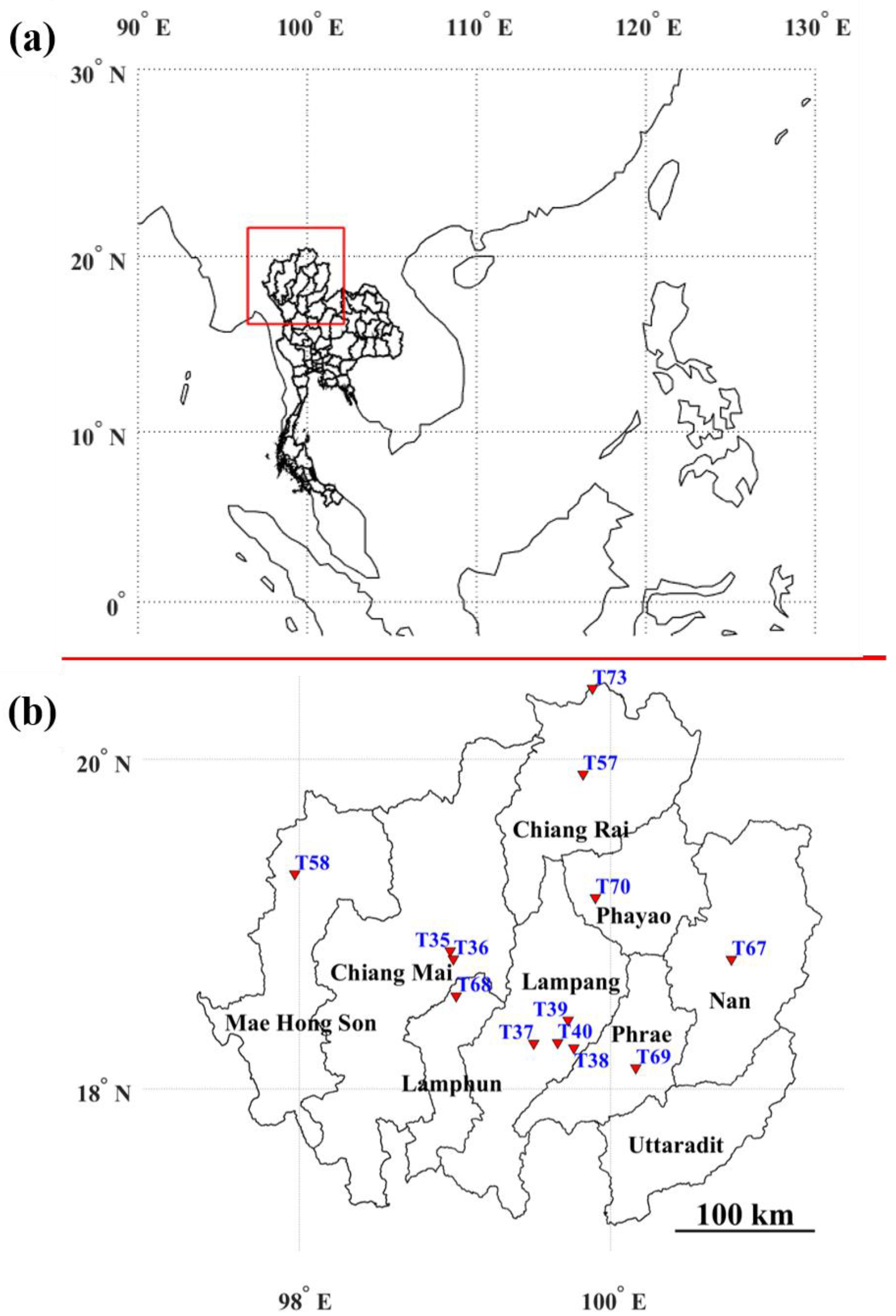
Figure 1.
(a) Overview of the study area, which is in the red box. (b) Locations of 13 PM10 concentration measuring stations in the northern region of Thailand employed in this study, where black lines show boundaries of provinces.
Figure 1.
(a) Overview of the study area, which is in the red box. (b) Locations of 13 PM10 concentration measuring stations in the northern region of Thailand employed in this study, where black lines show boundaries of provinces.
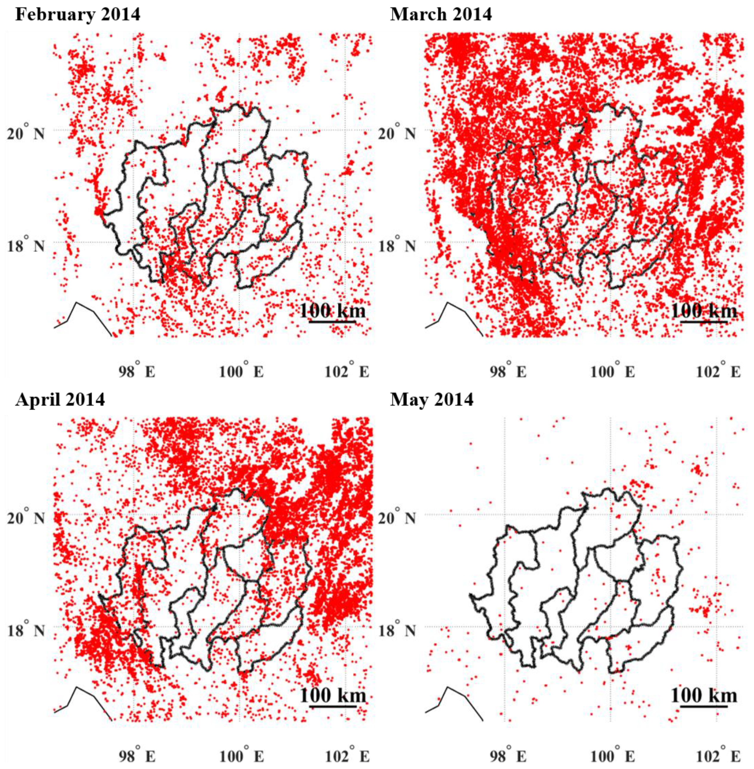
Figure 2.
All hotspots occurring in February–May of 2014 in the study area and neighboring regions.
Figure 2.
All hotspots occurring in February–May of 2014 in the study area and neighboring regions.
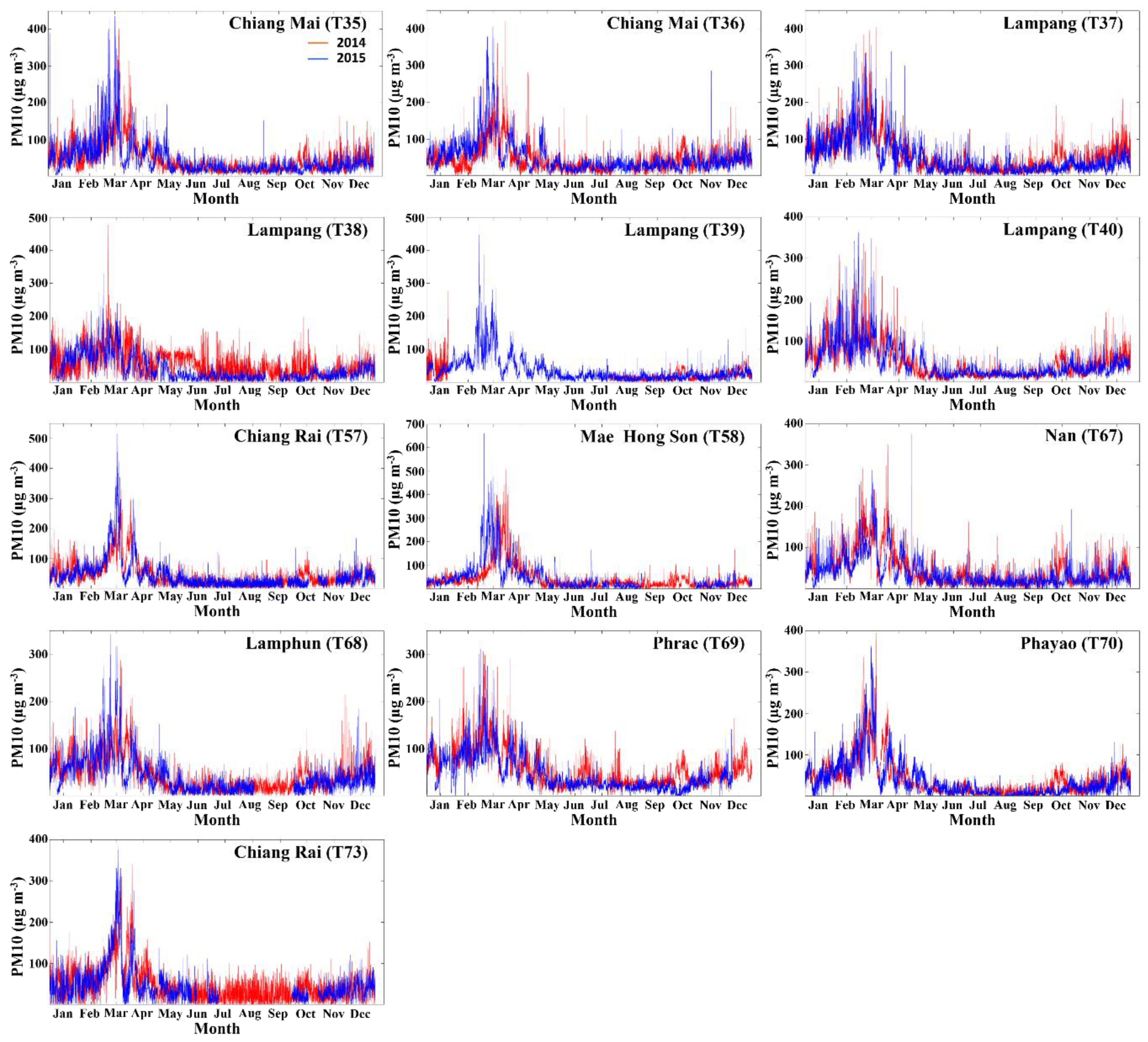
Figure 3.
Time series of measured hourly average PM10 concentrations (µg m−3) covering the whole years of 2014 (red) and 2015 (blue) for 13 stations employed in this study.
Figure 3.
Time series of measured hourly average PM10 concentrations (µg m−3) covering the whole years of 2014 (red) and 2015 (blue) for 13 stations employed in this study.
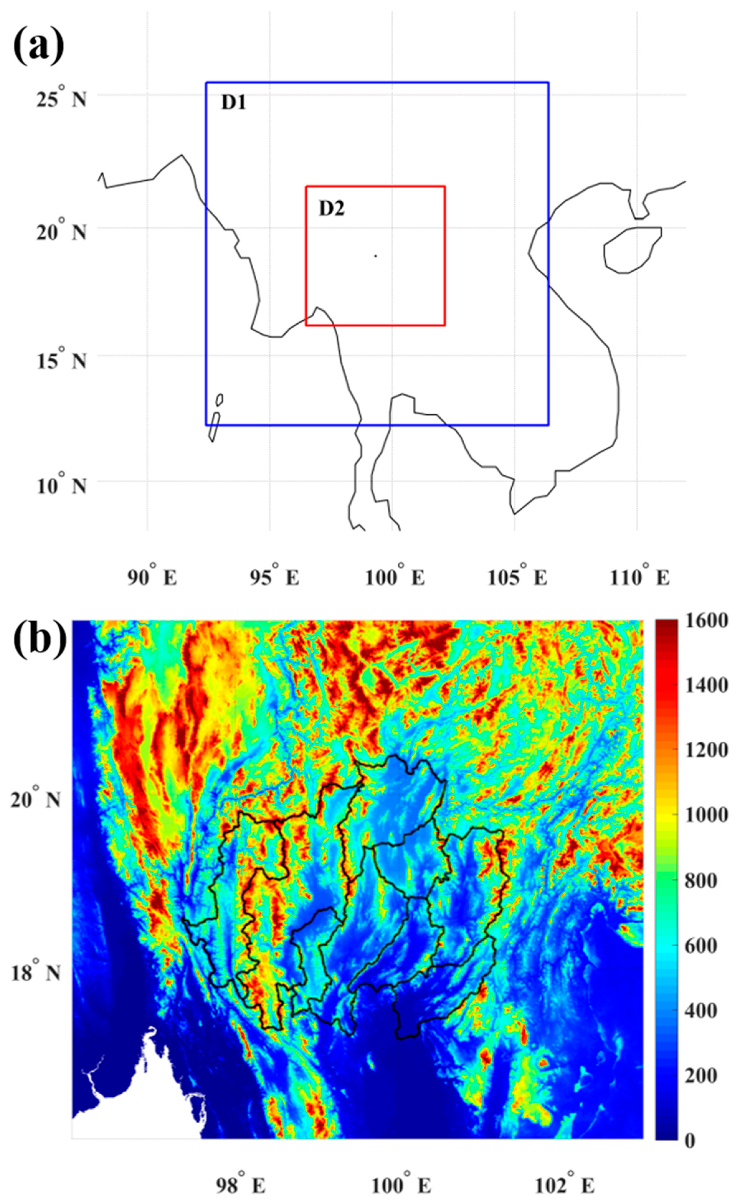
Figure 4.
(a) Coverages of two nested WRF domains employed in this study. (b) Topography (m) above mean sea level of WRF domain 2.
Figure 4.
(a) Coverages of two nested WRF domains employed in this study. (b) Topography (m) above mean sea level of WRF domain 2.
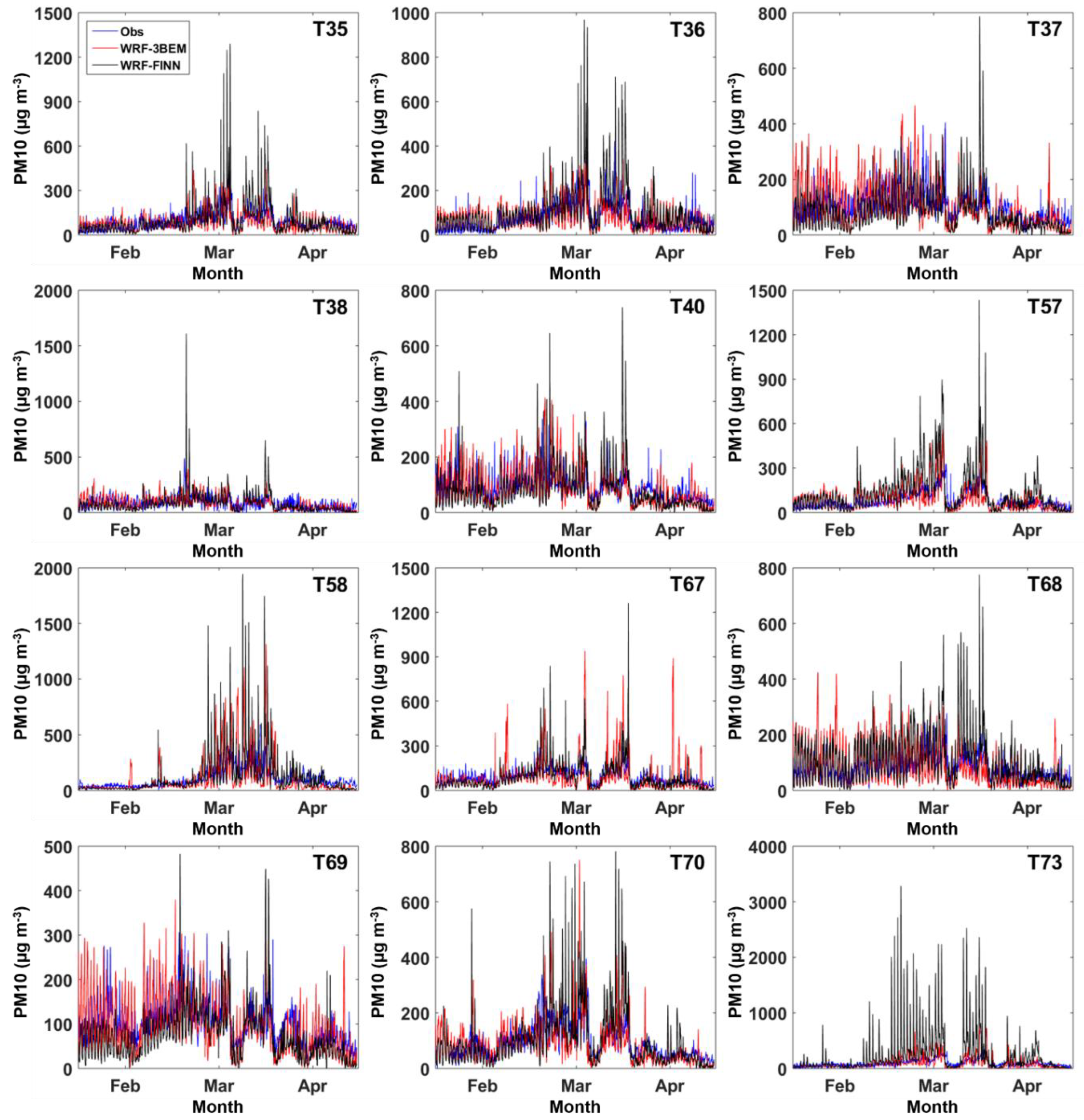
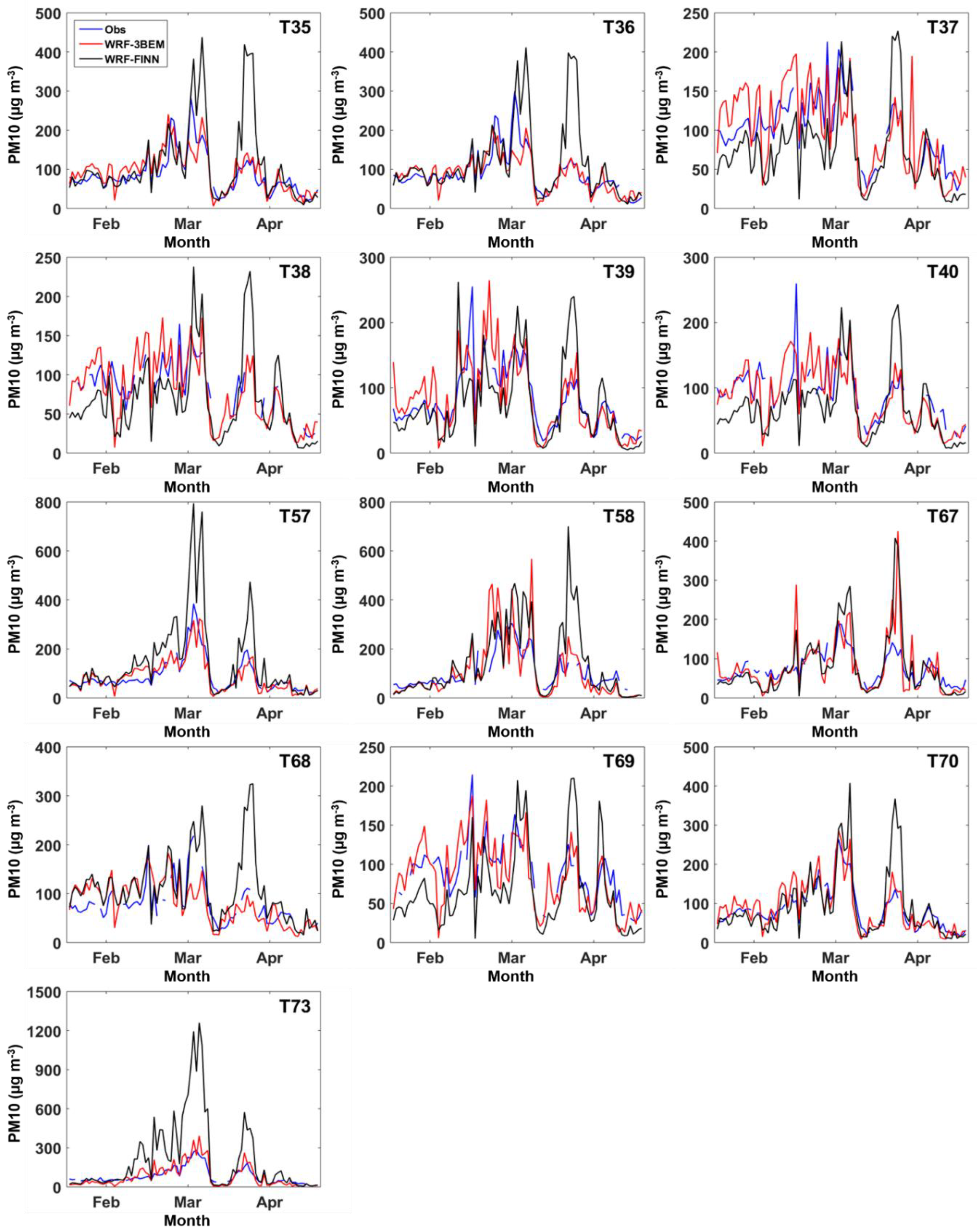
Figure 5.
Comparisons of time series of measured hourly average PM10 concentrations (μg m−3) and simulations of WRF-3BEM and WRF-FINN for February–April in 2014 for 12 ground stations.
Figure 5.
Comparisons of time series of measured hourly average PM10 concentrations (μg m−3) and simulations of WRF-3BEM and WRF-FINN for February–April in 2014 for 12 ground stations.
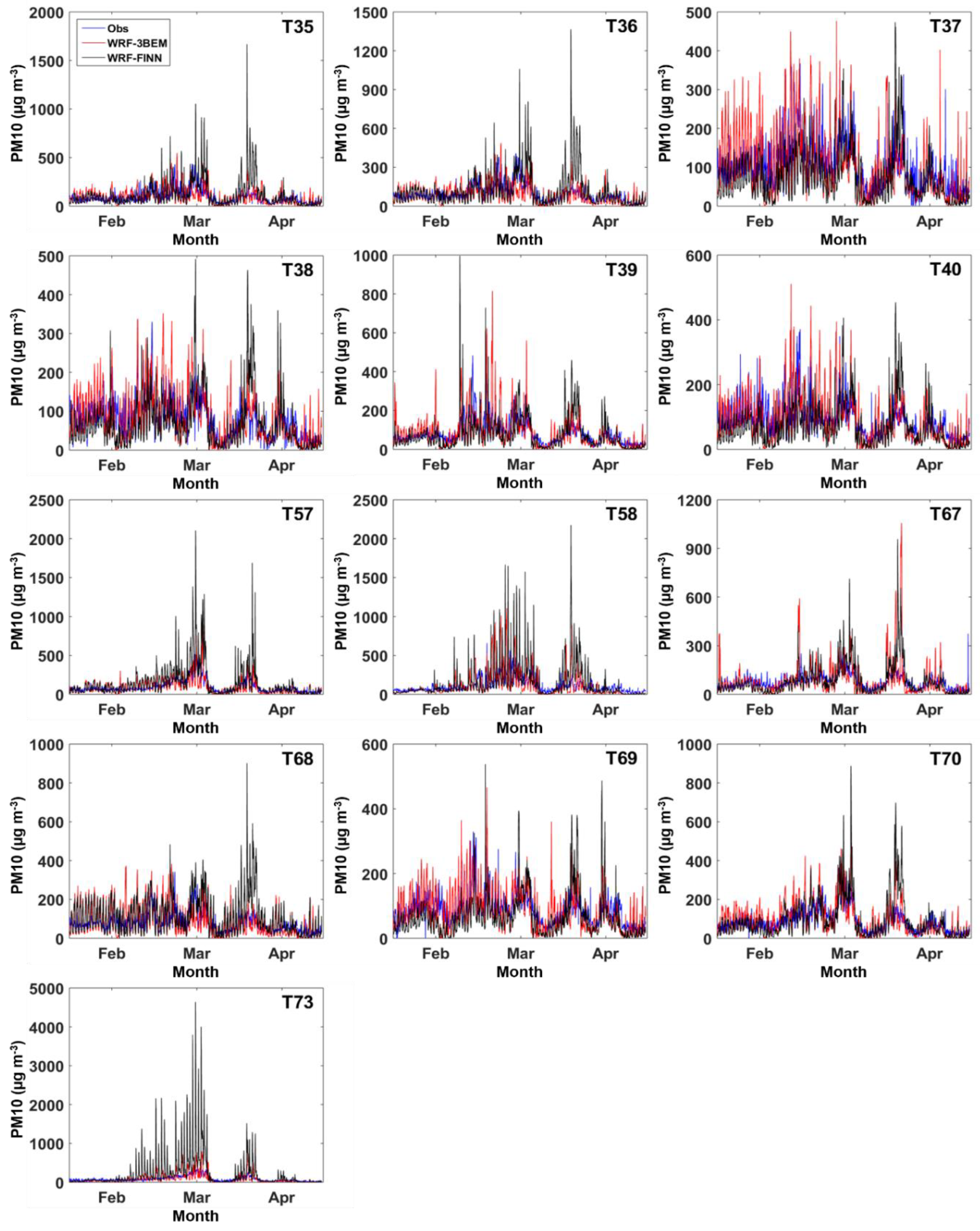
Figure 6.
Comparisons of time series of measured hourly average PM10 concentrations (μg m−3) and simulations of WRF-3BEM and WRF-FINN for February–April in 2015 for 13 ground stations.
Figure 6.
Comparisons of time series of measured hourly average PM10 concentrations (μg m−3) and simulations of WRF-3BEM and WRF-FINN for February–April in 2015 for 13 ground stations.
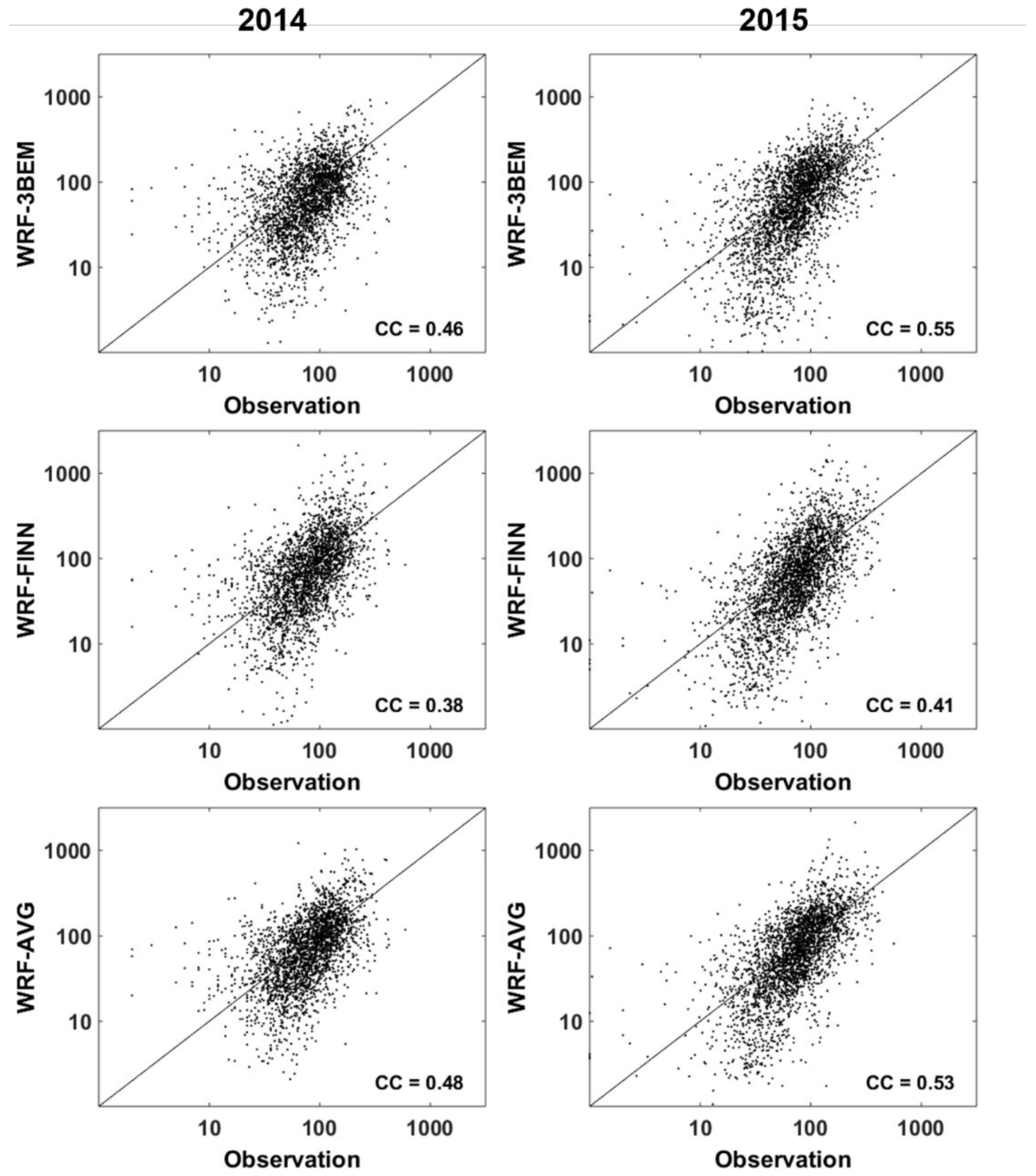
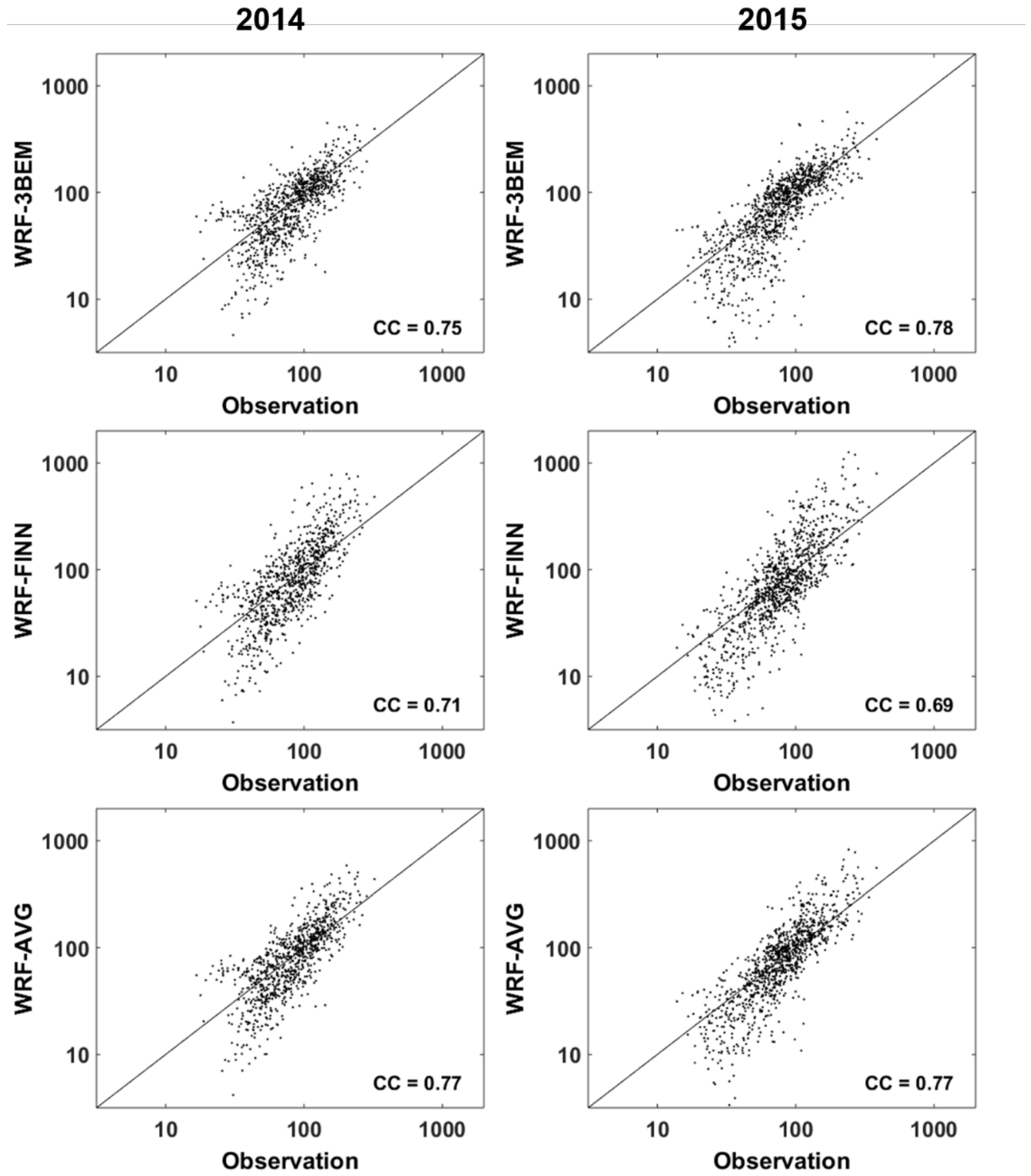
Figure 7.
Scatter plots comparing measured hourly average PM10 concentrations (μg m−3) and simulations of WRF-3BEM, WRF-FINN, and WRF-AVG for February–April in 2014 and 2015 for all ground stations.
Figure 7.
Scatter plots comparing measured hourly average PM10 concentrations (μg m−3) and simulations of WRF-3BEM, WRF-FINN, and WRF-AVG for February–April in 2014 and 2015 for all ground stations.
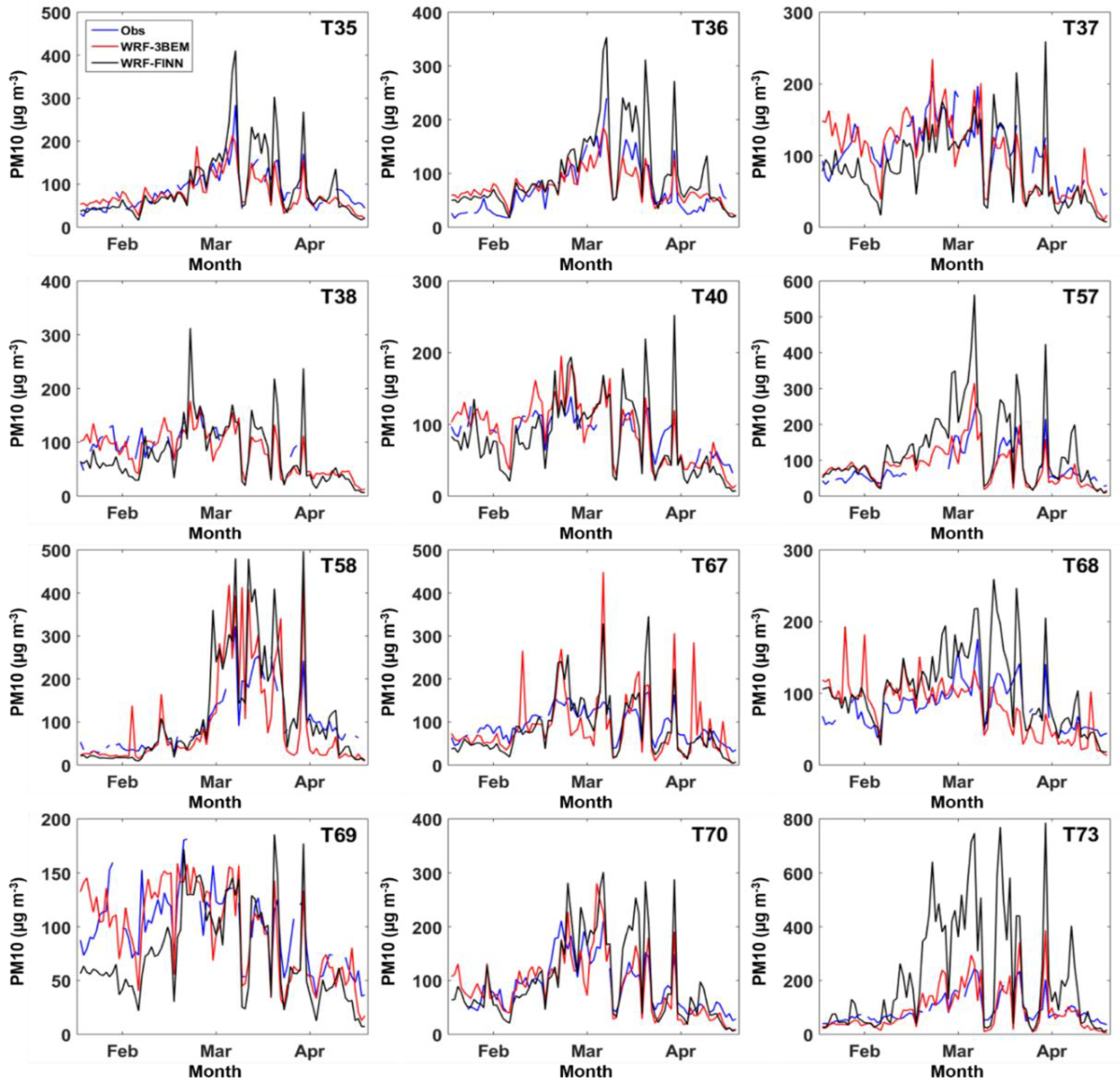
Figure 8.
Comparisons of time series of measured daily average PM10 concentrations (μg m−3) and simulations of WRF-3BEM and WRF-FINN for February–April in 2014 for 12 ground stations.
Figure 8.
Comparisons of time series of measured daily average PM10 concentrations (μg m−3) and simulations of WRF-3BEM and WRF-FINN for February–April in 2014 for 12 ground stations.
Figure 9.
Comparisons of time series of measured daily average PM10 concentrations (μg m−3) and simulations of WRF-3BEM and WRF-FINN for February–April in 2015 for 13 ground stations.
Figure 9.
Comparisons of time series of measured daily average PM10 concentrations (μg m−3) and simulations of WRF-3BEM and WRF-FINN for February–April in 2015 for 13 ground stations.
Figure 10.
Scatter plots comparing measured daily average PM10 concentrations (μg m−3) and simulations of WRF-3BEM, WRF-FINN, and WRF-AVG for February–April 2014 and 2015 for all ground stations.
Figure 10.
Scatter plots comparing measured daily average PM10 concentrations (μg m−3) and simulations of WRF-3BEM, WRF-FINN, and WRF-AVG for February–April 2014 and 2015 for all ground stations.
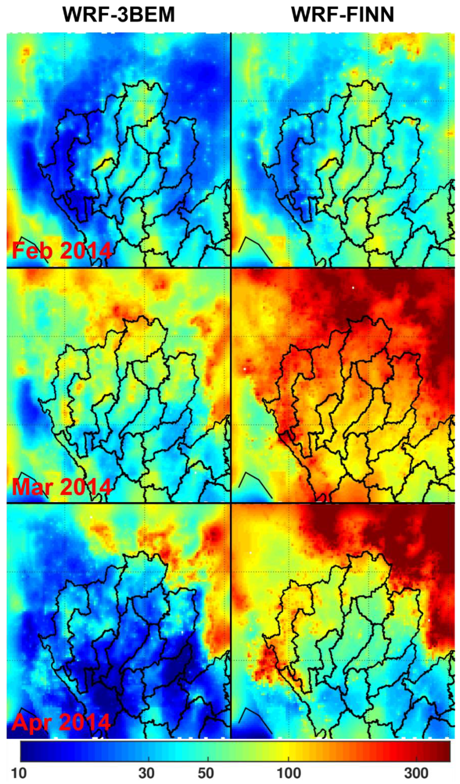
Figure 11.
Comparisons of simulated monthly average PM10 concentrations (μg m−3) at 2 m above ground of WRF-3BEM and WRF-FINN. Top to bottom are February, March, and April of 2014.
Figure 11.
Comparisons of simulated monthly average PM10 concentrations (μg m−3) at 2 m above ground of WRF-3BEM and WRF-FINN. Top to bottom are February, March, and April of 2014.
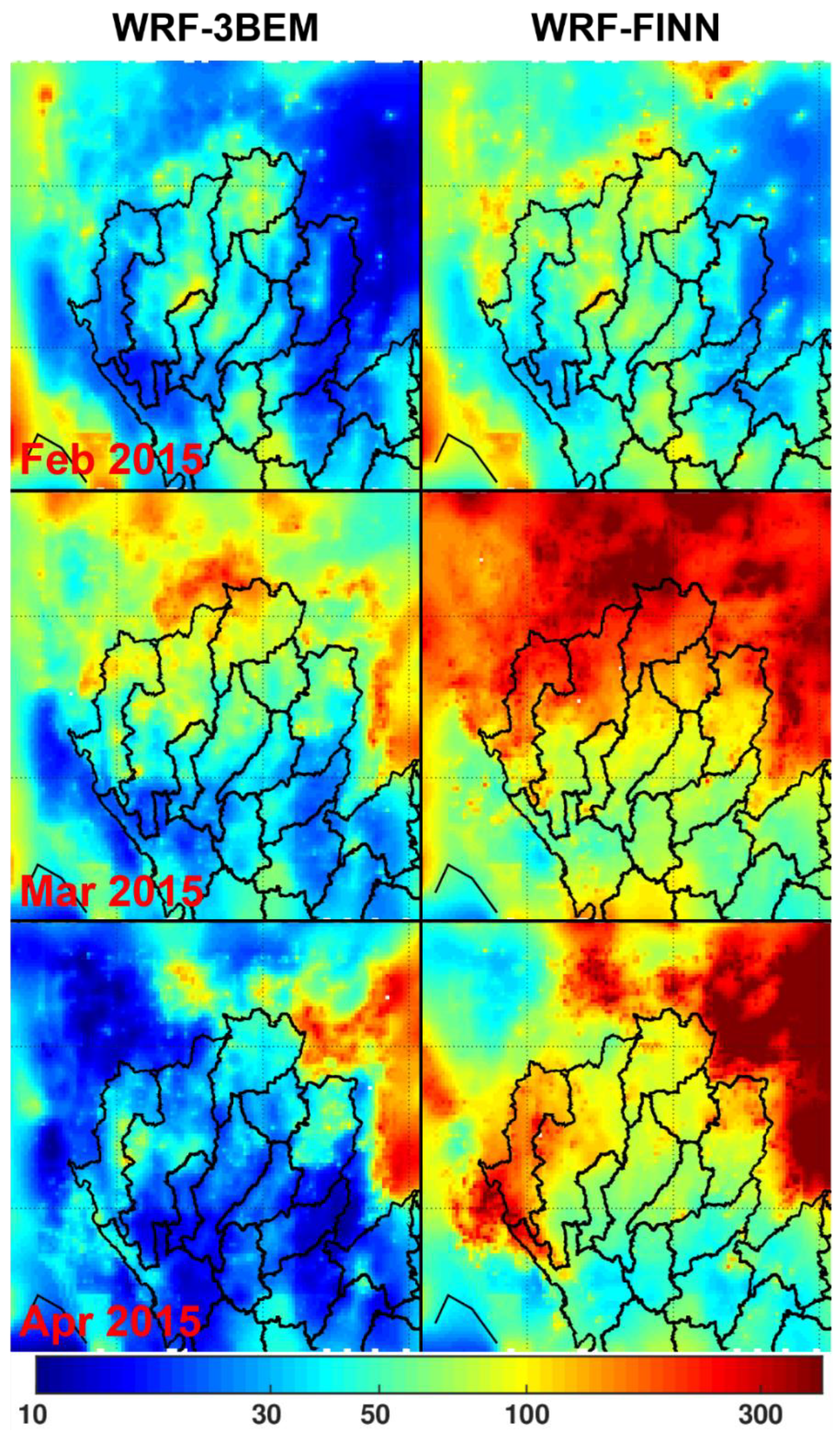
Figure 12.
Comparisons of simulated monthly average PM10 concentrations (μg m−3) at 2 m above ground of WRF-3BEM and WRF-FINN. Top to bottom are February, March, and April of 2015.
Figure 12.
Comparisons of simulated monthly average PM10 concentrations (μg m−3) at 2 m above ground of WRF-3BEM and WRF-FINN. Top to bottom are February, March, and April of 2015.
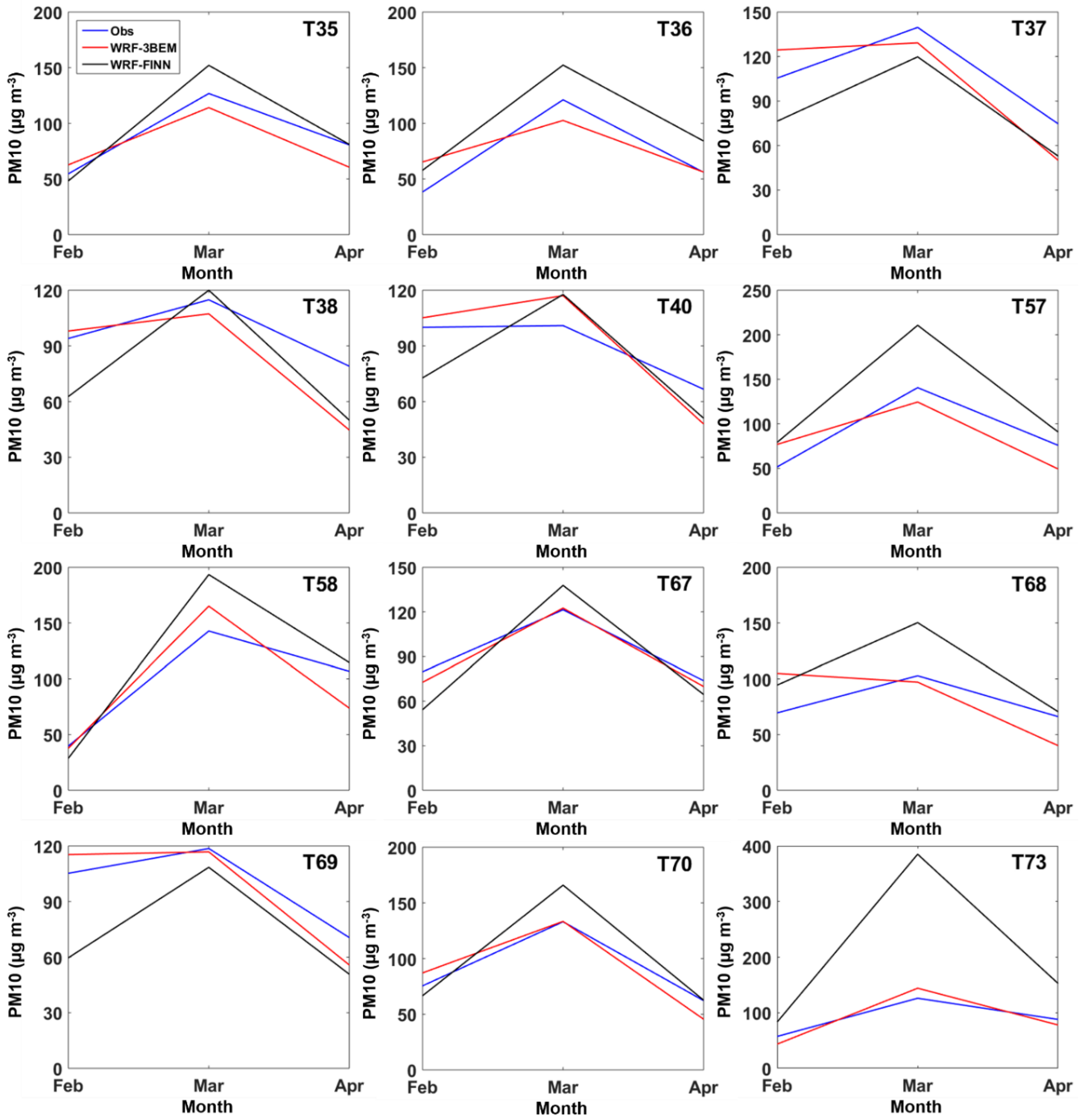
Figure 13.
Comparisons of measured monthly average PM10 concentrations (μg m−3) and simulations of WRF-3BEM and WRF-FINN for February–April 2014 for 12 ground stations.
Figure 13.
Comparisons of measured monthly average PM10 concentrations (μg m−3) and simulations of WRF-3BEM and WRF-FINN for February–April 2014 for 12 ground stations.
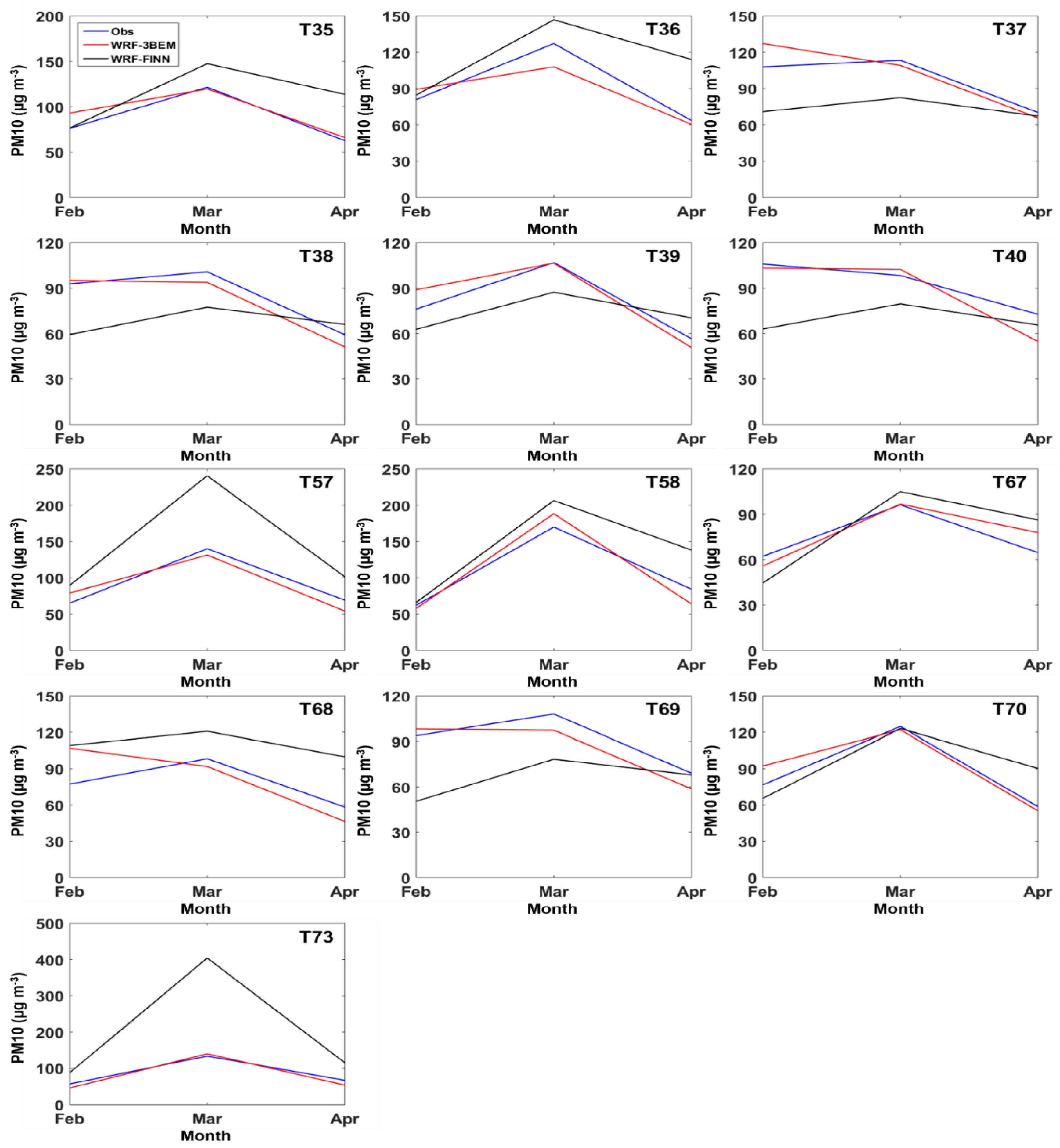
Figure 14.
Comparisons of measured monthly average PM10 concentrations (μg m−3) and simulations of WRF-3BEM and WRF-FINN for February–April 2015 for 13 ground stations.
Figure 14.
Comparisons of measured monthly average PM10 concentrations (μg m−3) and simulations of WRF-3BEM and WRF-FINN for February–April 2015 for 13 ground stations.
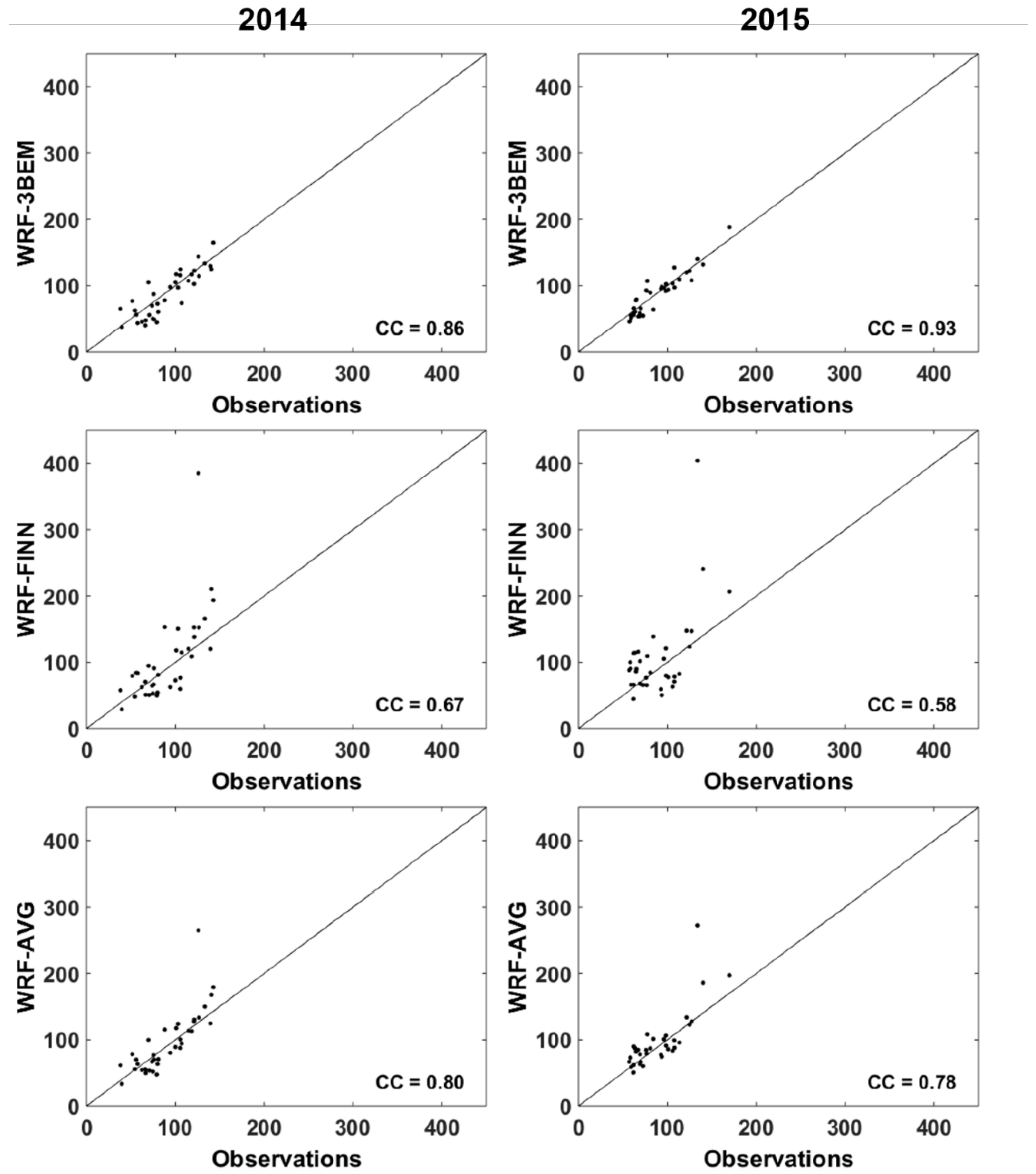
Figure 15.
Scatter plots comparing measured monthly average PM10 concentrations (μg m−3) and simulations of WRF-3BEM, WRF-FINN, and WRF-AVG for February–April 2014 and 2015.
Figure 15.
Scatter plots comparing measured monthly average PM10 concentrations (μg m−3) and simulations of WRF-3BEM, WRF-FINN, and WRF-AVG for February–April 2014 and 2015.
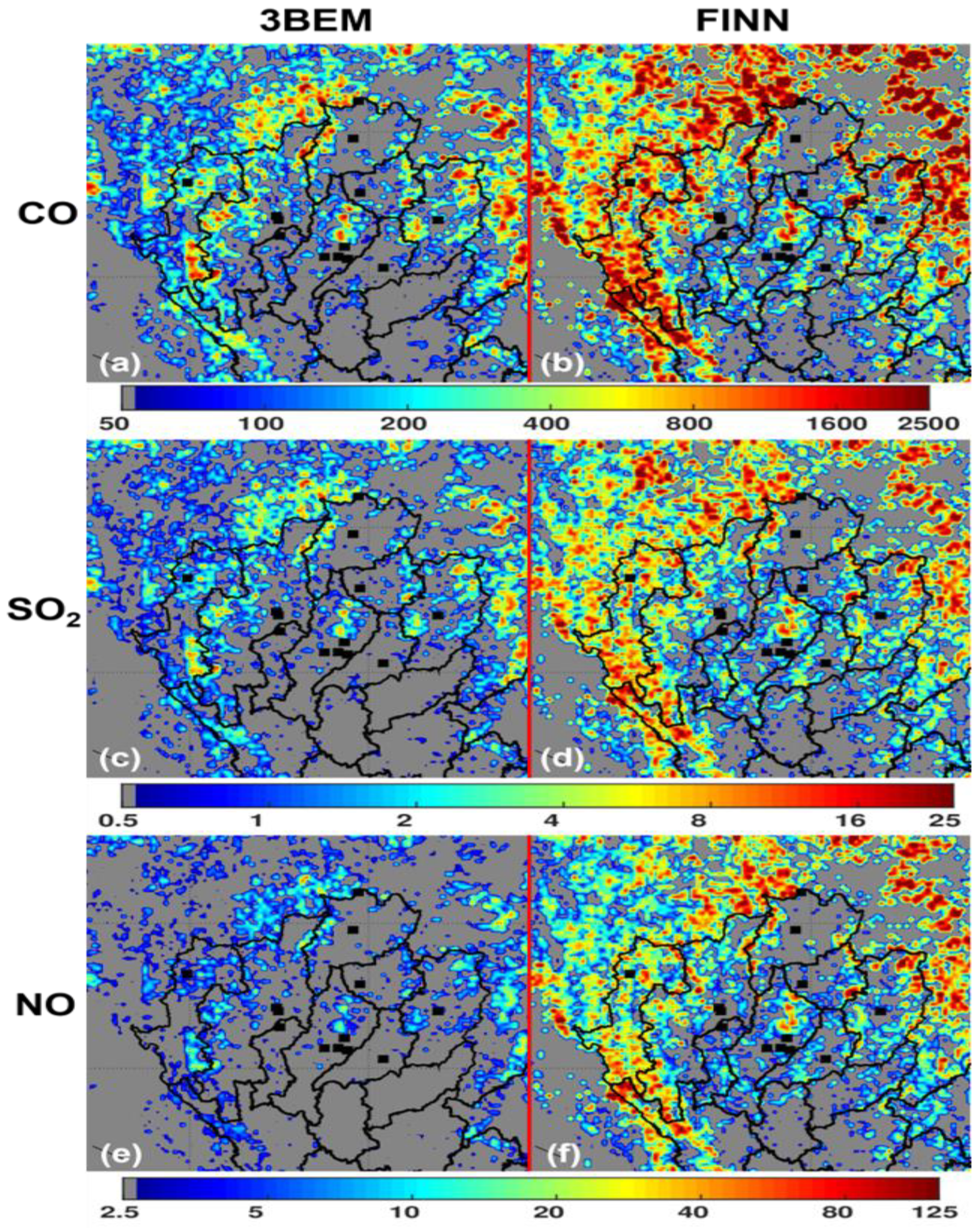
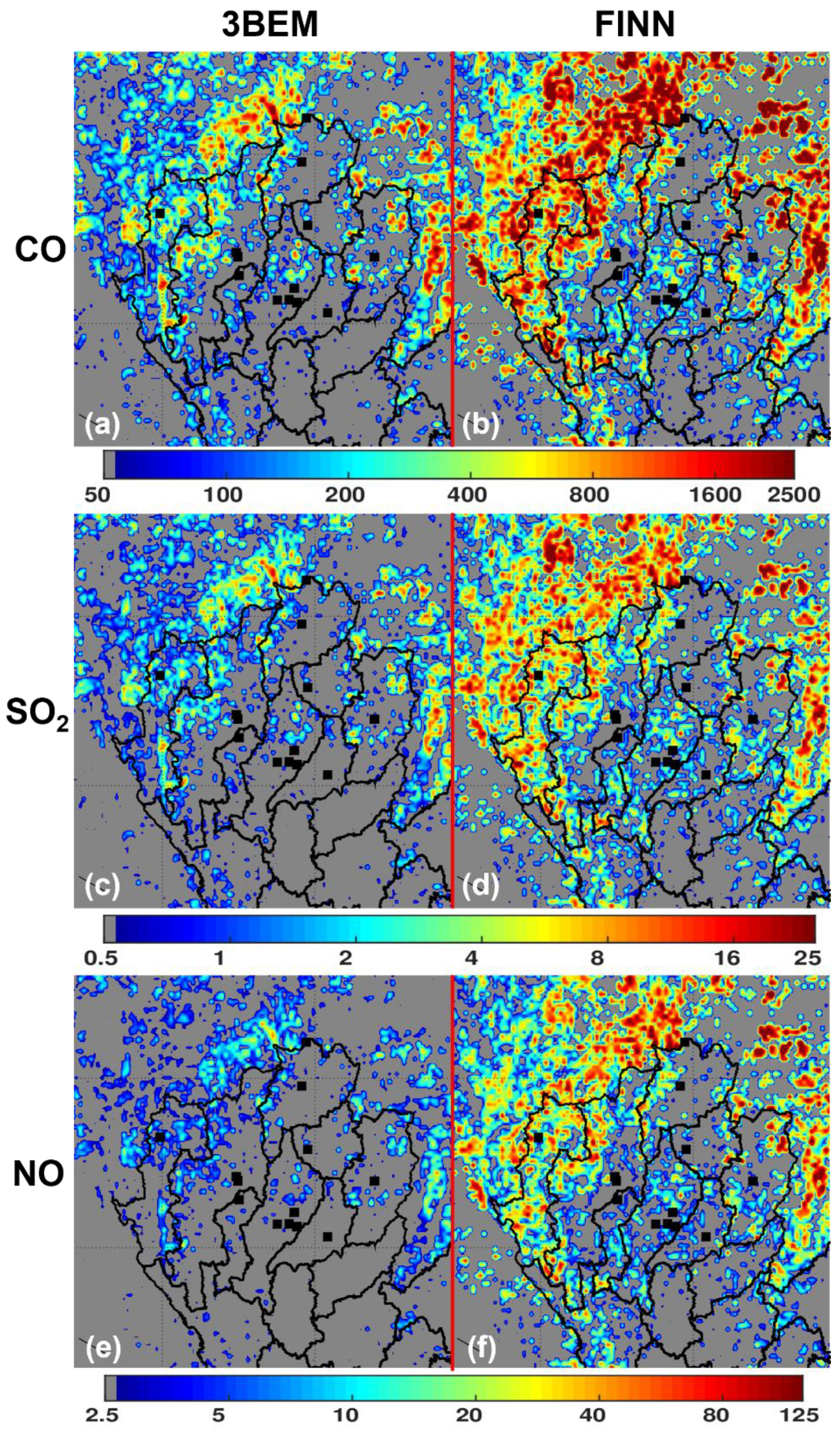
Figure 16.
Comparisons of daily total 3BEM (a,c,e) and FINN (b,d,f) emissions (kg m−2 day−1) over the study area averaged over 31 days in March 2014. Top to bottom rows: CO, SO2, and NO emissions, respectively. Black squares in each sub-figure show locations of ground stations employed in this study.
Figure 17.
Comparisons of daily total 3BEM (a,c,e) and FINN (b,d,f) emissions (kg m−2 day−1) over the study area averaged over 31 days in March 2015. Top to bottom rows: CO, SO2, and NO emissions, respectively. The black squares in each sub-figure show the locations of ground stations employed in this study.
Table 1.
Latitude, longitude, province, land use category, topography (m) above mean sea level, dates when the peak daily average PM10 concentrations occurred in 2014 and 2015, and the peak daily average PM10 concentrations for both years for the 13 ground stations.
Table 1.
Latitude, longitude, province, land use category, topography (m) above mean sea level, dates when the peak daily average PM10 concentrations occurred in 2014 and 2015, and the peak daily average PM10 concentrations for both years for the 13 ground stations.
| Station | Latitude | Longitude | Province | Land Use Category | Topography (m) | Peak of Daily Average PM10 Concentration |
|---|
| Month/Date | Values (µg m−3) |
|---|
| 2014 | 2015 | 2014 | 2015 |
|---|
| T35 | 18.8406 | 98.9697 | Chiang Mai | Urban | 410.7 | 3/21 | 3/16 | 284.0 | 282.4 |
| T36 | 18.7911 | 98.9900 | Chiang Mai | Urban | 365.4 | 3/21 | 3/16 | 240.0 | 299.8 |
| T37 | 18.2783 | 99.5064 | Lampang | Urban | 274.2 | 3/7 | 3/12 | 204.3 | 213.2 |
| T38 | 18.2507 | 99.7640 | Lampang | Urban | 395.2 | 3/7 | 3/12 | 181.5 | 165.0 |
| T39 | 18.4197 | 99.7273 | Lampang | Agriculture | 409.5 | N/A | 3/1 | N/A | 255.3 |
| T40 | 18.2827 | 99.6599 | Lampang | Forest | 377.15 | 3/10 | 3/1 | 138.7 | 260.0 |
| T57 | 19.9092 | 99.8234 | Chiang Rai | Urban | 381.4 | 3/21 | 3/17 | 263.3 | 384.0 |
| T58 | 19.3047 | 97.9710 | Mae Hong Son | Urban | 410.7 | 3/21 | 3/15 | 322.7 | 304.0 |
| T67 | 18.7889 | 100.7764 | Nan | Urban | 224.6 | 3/3 | 3/16 | 169.7 | 189.2 |
| T68 | 18.5674 | 99.0080 | Lamphun | Urban | 287.75 | 3/21 | 3/17 | 175.6 | 218.2 |
| T69 | 18.1289 | 100.1623 | Phrae | Urban | 183.7 | 3/6 | 3/1 | 181.2 | 214.7 |
| T70 | 19.1639 | 99.9027 | Phayao | Urban | 385.85 | 3/7 | 3/16 | 211.0 | 263.5 |
| T73 | 20.4272 | 99.8837 | Chiang Rai | Urban | 510.9 | 3/20 | 3/18 | 244.9 | 282.6 |
Table 2.
WRF-Chem domain configurations and physics options employed in this study.
Table 2.
WRF-Chem domain configurations and physics options employed in this study.
| Configuration | Domain 1 | Domain 2 |
|---|
| Grid Size | 99 × 99 | 120 × 120 |
| Spatial Resolution (km) | 15 | 5 |
| Number of Vertical Levels | 45 | 45 |
| Microphysics Scheme | WRF Double-Moment 6-class | WRF Double-Moment 6-class |
| Cumulus Parameterization Scheme | Grell 3D Ensemble Scheme | Grell 3D Ensemble Scheme |
| Planetary Boundary Layer (PBL) scheme | Bretherton and Park | Bretherton and Park |
| Surface Layer Scheme | Revised MM5 Monin-Obukhov | Revised MM5 Monin-Obukhov |
| Land Surface Model | Unified Noah | Unified Noah |
| Aerosol Scheme | Goddard Chemistry Aerosol Radiation and Transport | Goddard Chemistry Aerosol Radiation and Transport |
Table 3.
MEs (E[simulations-measurements]), RMSEs, and CCs of simulations and measurements for WRF-3BEM, WRF-FINN, and WRF-AVG simulated hourly average PM10 concentrations (μg m−3) for February–April of 2014 evaluated using measurements from 12 ground stations. (CC: correlation coefficient, RMSE: root mean squared error).
| Station | WRF-3BEM | WRF-FINN | WRF-AVG |
|---|
| ME | RMSE | CC | ME | RMSE | CC | ME | RMSE | CC |
|---|
| T35 | −7.65 | 66.71 | 0.38 | 8.57 | 101.00 | 0.45 | 0.46 | 70.48 | 0.48 |
| T36 | 4.22 | 60.03 | 0.44 | 29.40 | 93.26 | 0.48 | 16.81 | 65.26 | 0.52 |
| T37 | −4.88 | 84.80 | 0.22 | −22.56 | 73.12 | 0.44 | −13.72 | 69.62 | 0.37 |
| T38 | −4.38 | 58.36 | 0.45 | −10.01 | 88.65 | 0.27 | −7.19 | 63.01 | 0.40 |
| T40 | 0.78 | 55.29 | 0.55 | −7.39 | 71.35 | 0.38 | −3.30 | 53.44 | 0.53 |
| T57 | 2.48 | 70.66 | 0.49 | 49.62 | 122.67 | 0.63 | 26.05 | 83.29 | 0.63 |
| T58 | −1.90 | 130.04 | 0.56 | 19.38 | 167.88 | 0.41 | 8.74 | 121.12 | 0.56 |
| T67 | −1.52 | 102.71 | 0.41 | −3.77 | 71.80 | 0.65 | −2.64 | 71.93 | 0.60 |
| T68 | −1.26 | 66.05 | 0.36 | 26.54 | 81.63 | 0.49 | 12.64 | 62.32 | 0.49 |
| T69 | −2.08 | 62.58 | 0.37 | −24.35 | 59.87 | 0.43 | −13.22 | 53.99 | 0.44 |
| T70 | −4.75 | 68.39 | 0.57 | 8.16 | 91.29 | 0.49 | 1.71 | 68.52 | 0.58 |
| T73 | −1.22 | 94.79 | 0.54 | 119.46 | 343.72 | 0.40 | 59.12 | 191.59 | 0.48 |
| All | −1.83 | 79.84 | 0.46 | 16.43 | 137.24 | 0.38 | 7.30 | 89.92 | 0.48 |
Table 4.
MEs (E[simulations-measurements]), RMSEs, and CCs of simulations and measurements for WRF-3BEM, WRF-FINN, and WRF-AVG simulated hourly average PM10 concentrations (μg m−3) for February–April of 2015 evaluated using measurements from 13 ground stations.
Table 4.
MEs (E[simulations-measurements]), RMSEs, and CCs of simulations and measurements for WRF-3BEM, WRF-FINN, and WRF-AVG simulated hourly average PM10 concentrations (μg m−3) for February–April of 2015 evaluated using measurements from 13 ground stations.
| Station | WRF-3BEM | WRF-FINN | WRF-AVG |
|---|
| ME | RMSE | CC | ME | RMSE | CC | ME | RMSE | CC |
|---|
| T35 | 5.97 | 78.76 | 0.41 | 26.97 | 124.99 | 0.42 | 16.47 | 86.17 | 0.47 |
| T36 | −5.05 | 67.25 | 0.50 | 25.59 | 114.44 | 0.46 | 10.27 | 75.73 | 0.54 |
| T37 | 2.46 | 76.93 | 0.44 | −23.90 | 69.70 | 0.44 | −10.72 | 62.27 | 0.50 |
| T38 | 0.25 | 49.41 | 0.60 | −11.54 | 62.22 | 0.43 | −5.65 | 46.60 | 0.59 |
| T39 | 1.01 | 63.72 | 0.63 | −6.82 | 77.63 | 0.43 | −2.90 | 56.25 | 0.63 |
| T40 | −3.16 | 63.09 | 0.50 | −19.78 | 67.65 | 0.39 | −11.47 | 55.66 | 0.52 |
| T57 | −2.70 | 74.19 | 0.64 | 54.78 | 170.95 | 0.64 | 26.04 | 105.94 | 0.68 |
| T58 | 2.45 | 130.20 | 0.58 | 35.78 | 209.88 | 0.31 | 19.11 | 141.79 | 0.50 |
| T67 | 2.52 | 91.87 | 0.43 | 5.23 | 73.02 | 0.65 | 3.88 | 71.14 | 0.60 |
| T68 | 2.90 | 69.26 | 0.40 | 31.79 | 86.77 | 0.52 | 17.34 | 65.72 | 0.53 |
| T69 | −2.20 | 53.79 | 0.53 | −19.91 | 63.11 | 0.44 | −11.05 | 49.79 | 0.55 |
| T70 | 2.68 | 59.59 | 0.69 | 7.08 | 79.21 | 0.63 | 4.88 | 61.22 | 0.70 |
| T73 | 0.83 | 92.98 | 0.64 | 128.47 | 401.57 | 0.52 | 64.65 | 220.68 | 0.60 |
| All | 0.63 | 77.32 | 0.55 | 18.17 | 153.50 | 0.41 | 9.40 | 96.55 | 0.53 |
Table 5.
Overall MEs (E[simulations-measurements]), RMSEs, and CCs of simulations and measurements for WRF-3BEM, WRF-FINN, and WRF-AVG simulated hourly, daily, and monthly average PM10 concentrations (μg m−3) for February–April of 2014 and 2015 evaluated using measurements from all 12 ground stations.
| PM10 | WRF-3BEM | WRF-FINN | WRF-AVG |
|---|
| ME | RMSE | CC | ME | RMSE | CC | ME | RMSE | CC |
|---|
| Hourly | −0.54 | 78.52 | 0.51 | 17.34 | 146.00 | 0.40 | 8.40 | 93.46 | 0.50 |
| Daily | −0.18 | 40.94 | 0.76 | 19.03 | 92.23 | 0.70 | 9.43 | 56.79 | 0.77 |
| Monthly | −2.02 | 14.81 | 0.89 | 14.13 | 52.87 | 0.63 | 6.06 | 27.95 | 0.79 |
Table 6.
MEs (E[simulations-measurements]), RMSEs, and CCs of simulations and measurements for WRF-3BEM, WRF-FINN, and WRF-AVG simulated daily average PM10 concentrations (μg m−3) for February–April of 2014 evaluated using measurements from 12 ground stations.
Table 6.
MEs (E[simulations-measurements]), RMSEs, and CCs of simulations and measurements for WRF-3BEM, WRF-FINN, and WRF-AVG simulated daily average PM10 concentrations (μg m−3) for February–April of 2014 evaluated using measurements from 12 ground stations.
| Station | WRF-3BEM | WRF-FINN | WRF-AVG |
|---|
| ME | RMSE | CC | ME | RMSE | CC | ME | RMSE | CC |
|---|
| T35 | −7.54 | 27.92 | 0.81 | 8.88 | 45.40 | 0.90 | 0.67 | 28.43 | 0.89 |
| T36 | 5.48 | 29.20 | 0.82 | 31.95 | 50.65 | 0.87 | 18.71 | 30.94 | 0.88 |
| T37 | −2.87 | 38.63 | 0.65 | −22.11 | 43.43 | 0.68 | −12.49 | 35.54 | 0.71 |
| T38 | −3.75 | 27.95 | 0.56 | −15.18 | 40.15 | 0.69 | −9.47 | 29.14 | 0.69 |
| T40 | 1.61 | 26.75 | 0.82 | −4.69 | 39.07 | 0.74 | −1.54 | 29.20 | 0.82 |
| T57 | 2.01 | 38.15 | 0.76 | 50.99 | 87.69 | 0.88 | 26.50 | 53.08 | 0.86 |
| T58 | −2.73 | 64.84 | 0.83 | −22.01 | 78.20 | 0.88 | 9.64 | 63.59 | 0.89 |
| T67 | −4.43 | 56.99 | 0.65 | −3.68 | 44.85 | 0.86 | −4.06 | 46.20 | 0.79 |
| T68 | −1.21 | 35.51 | 0.44 | 27.47 | 44.06 | 0.84 | 13.13 | 30.25 | 0.75 |
| T69 | −1.48 | 28.94 | 0.73 | −24.94 | 38.73 | 0.73 | −13.21 | 27.90 | 0.79 |
| T70 | −3.77 | 35.06 | 0.81 | 9.67 | 49.03 | 0.83 | 2.95 | 36.88 | 0.85 |
| T73 | −2.05 | 46.15 | 0.85 | 116.06 | 206.60 | 0.81 | 57.01 | 117.52 | 0.84 |
| All | −1.77 | 40.38 | 0.75 | 18.19 | 81.32 | 0.71 | 8.21 | 51.98 | 0.77 |
Table 7.
MEs (E[simulations-measurements]), RMSEs, and CCs of simulations and measurements for WRF-3BEM, WRF-FINN, and WRF-AVG simulated daily average PM10 concentrations (μg m−3) for February–April of 2015 evaluated using measurements from 13 ground stations.
Table 7.
MEs (E[simulations-measurements]), RMSEs, and CCs of simulations and measurements for WRF-3BEM, WRF-FINN, and WRF-AVG simulated daily average PM10 concentrations (μg m−3) for February–April of 2015 evaluated using measurements from 13 ground stations.
| Station | WRF-3BEM | WRF-FINN | WRF-AVG |
|---|
| ME | RMSE | CC | ME | RMSE | CC | ME | RMSE | CC |
|---|
| T35 | 6.71 | 33.66 | 0.79 | 27.43 | 78.33 | 0.72 | 17.07 | 46.07 | 0.80 |
| T36 | −5.02 | 34.31 | 0.78 | 26.68 | 75.85 | 0.68 | 10.83 | 43.13 | 0.77 |
| T37 | 4.53 | 35.15 | 0.74 | −25.21 | 42.08 | 0.75 | −10.34 | 27.91 | 0.83 |
| T38 | 0.24 | 25.38 | 0.78 | −13.70 | 43.42 | 0.59 | −6.73 | 28.07 | 0.75 |
| T39 | 0.68 | 31.86 | 0.80 | −5.95 | 44.92 | 0.69 | −2.64 | 32.96 | 0.79 |
| T40 | −2.95 | 33.19 | 0.71 | −21.69 | 46.62 | 0.58 | −12.32 | 33.21 | 0.72 |
| T57 | −2.32 | 36.73 | 0.87 | 55.38 | 116.49 | 0.89 | 26.53 | 64.59 | 0.90 |
| T58 | 2.35 | 82.30 | 0.78 | 36.41 | 106.69 | 0.80 | 19.38 | 81.23 | 0.84 |
| T67 | 3.98 | 54.09 | 0.68 | 6.64 | 58.02 | 0.78 | 5.31 | 51.63 | 0.76 |
| T68 | 3.87 | 37.89 | 0.60 | 28.34 | 51.18 | 0.74 | 16.11 | 34.20 | 0.77 |
| T69 | −3.54 | 27.24 | 0.79 | −21.70 | 43.85 | 0.65 | −12.62 | 29.49 | 0.78 |
| T70 | 2.97 | 31.17 | 0.87 | 5.62 | 52.70 | 0.80 | 4.29 | 36.03 | 0.87 |
| T73 | 3.60 | 43.74 | 0.90 | 148.01 | 276.50 | 0.92 | 75.81 | 152.92 | 0.92 |
| All | 1.22 | 41.42 | 0.78 | 19.76 | 100.80 | 0.69 | 10.49 | 60.69 | 0.77 |
Table 8.
MEs (E[simulations-measurements]), RMSEs, and CCs of simulations and measurements for WRF-3BEM, WRF-FINN, and WRF-AVG simulated monthly average PM10 concentrations (μg m−3) for February–April 2014 evaluated using measurements from 12 ground stations.
Table 8.
MEs (E[simulations-measurements]), RMSEs, and CCs of simulations and measurements for WRF-3BEM, WRF-FINN, and WRF-AVG simulated monthly average PM10 concentrations (μg m−3) for February–April 2014 evaluated using measurements from 12 ground stations.
| Station | WRF-3BEM | WRF-FINN | WRF-AVG |
|---|
| ME | RMSE | CC | ME | RMSE | CC | ME | RMSE | CC |
|---|
| T35 | −8.23 | 14.46 | 0.92 | 6.45 | 15.09 | 1.00 | −0.89 | 6.76 | 0.98 |
| T36 | 2.87 | 18.93 | 0.92 | 26.25 | 26.71 | 1.00 | 14.56 | 16.12 | 1.00 |
| T37 | −5.34 | 18.89 | 0.88 | −23.56 | 23.89 | 0.99 | −14.45 | 16.24 | 0.98 |
| T38 | −12.64 | 20.45 | 0.89 | −18.40 | 24.86 | 0.97 | −15.52 | 19.95 | 1.00 |
| T40 | 0.85 | 14.58 | 0.99 | −8.70 | 20.55 | 0.77 | −3.93 | 15.14 | 0.92 |
| T57 | −5.80 | 23.13 | 0.80 | 37.53 | 44.29 | 0.98 | 15.86 | 22.05 | 0.94 |
| T58 | −4.26 | 23.05 | 0.91 | 15.81 | 30.26 | 0.99 | 5.78 | 22.61 | 0.96 |
| T67 | −3.29 | 4.71 | 1.00 | −6.12 | 18.33 | 0.97 | −4.71 | 11.35 | 0.99 |
| T68 | 1.18 | 25.55 | 0.48 | 25.61 | 31.07 | 0.98 | 13.39 | 22.06 | 0.82 |
| T69 | −2.17 | 10.39 | 0.97 | −25.17 | 29.29 | 0.81 | −13.67 | 14.72 | 0.99 |
| T70 | −1.58 | 11.73 | 0.95 | 8.13 | 19.67 | 0.99 | 3.28 | 10.70 | 1.00 |
| T73 | −1.91 | 14.32 | 0.99 | 116.57 | 154.88 | 0.97 | 57.33 | 81.60 | 0.98 |
| All | −3.36 | 17.67 | 0.86 | 12.87 | 51.61 | 0.67 | 4.75 | 28.58 | 0.80 |
Table 9.
MEs (E[simulations-measurements]), RMSEs, and CCs of simulations and measurements for WRF-3BEM, WRF-FINN, and WRF-AVG simulated monthly average PM10 concentrations (μg m−3) for February–April 2015 evaluated using measurements from 13 ground stations.
Table 9.
MEs (E[simulations-measurements]), RMSEs, and CCs of simulations and measurements for WRF-3BEM, WRF-FINN, and WRF-AVG simulated monthly average PM10 concentrations (μg m−3) for February–April 2015 evaluated using measurements from 13 ground stations.
| Station | WRF-3BEM | WRF-FINN | WRF-AVG |
|---|
| ME | RMSE | CC | ME | RMSE | CC | ME | RMSE | CC |
|---|
| T35 | 6.13 | 9.97 | 0.95 | 25.80 | 33.08 | 0.72 | 15.97 | 17.93 | 0.95 |
| T36 | −4.64 | 12.27 | 0.93 | 24.59 | 31.37 | 0.72 | 9.97 | 14.11 | 0.96 |
| T37 | 3.50 | 11.69 | 0.92 | −23.66 | 27.90 | 0.77 | −10.08 | 11.59 | 0.98 |
| T38 | −4.23 | 6.29 | 0.98 | −16.70 | 23.97 | 0.32 | −10.47 | 12.60 | 0.99 |
| T39 | 2.20 | 8.12 | 0.94 | −6.36 | 15.80 | 0.76 | −2.08 | 6.20 | 1.00 |
| T40 | −5.55 | 10.76 | 0.98 | −22.89 | 27.31 | 0.16 | −14.22 | 15.58 | 0.90 |
| T57 | −3.24 | 12.85 | 0.93 | 52.41 | 62.55 | 1.00 | 24.58 | 29.16 | 1.00 |
| T58 | −2.06 | 15.97 | 0.99 | 31.46 | 37.69 | 0.94 | 14.70 | 18.60 | 1.00 |
| T67 | 2.46 | 8.47 | 0.88 | 4.25 | 16.88 | 0.78 | 3.35 | 12.50 | 0.82 |
| T68 | 3.74 | 18.80 | 0.70 | 31.93 | 32.86 | 1.00 | 17.83 | 20.20 | 0.83 |
| T69 | −5.53 | 8.96 | 0.93 | −24.73 | 30.34 | 0.22 | −15.13 | 16.52 | 0.98 |
| T70 | 3.12 | 9.35 | 0.95 | 6.20 | 19.33 | 0.76 | 4.66 | 8.29 | 0.99 |
| T73 | −6.02 | 10.77 | 1.00 | 116.65 | 159.67 | 1.00 | 55.31 | 80.82 | 1.00 |
| All | −0.78 | 11.56 | 0.93 | 15.30 | 54.00 | 0.58 | 7.26 | 27.36 | 0.78 |
Table 10.
Daily total 3BEM and FINN emissions (kg m−2 day−1) of CO, SO2, and NO averaged over the study area and over 31 days in March of 2014 and 2015.
Table 10.
Daily total 3BEM and FINN emissions (kg m−2 day−1) of CO, SO2, and NO averaged over the study area and over 31 days in March of 2014 and 2015.
| Emission Species | March 2014 | March 2015 |
|---|
| 3BEM | FINN | 3BEM | FINN |
|---|
| CO | 154.06 | 498.15 | 133.08 | 440.06 |
| SO2 | 0.88 | 3.00 | 0.77 | 2.66 |
| NO | 2.14 | 12.88 | 1.83 | 11.30 |


