Article

Monitoring and Modeling Roof-Level Wind Speed in a Changing City

by
Kathrin Baumann-Stanzer
1,*,
Sirma Stenzel
1,
Gabriele Rau
1,
Martin Piringer
1,
Felix Feichtinger
2 and
Théophane Costabloz
3
1
Zentralanstalt für Meteorologie und Geodynamik, Hohe Warte 38, 1190 Vienna, Austria
2
Institut für Erneuerbare Energie, University of Applied Sciences (FH Technikum Wien), Höchstädtplatz 6, 1200 Vienna, Austria
3
École nationale de la météorologie, 42 Avenue Gaspard Coriolis, 31 057 Toulouse CEDEX, France
*
Author to whom correspondence should be addressed.
Atmosphere 2020, 11(1), 87; https://doi.org/10.3390/atmos11010087
Submission received: 13 November 2019 / Revised: 27 December 2019 / Accepted: 31 December 2019 / Published: 10 January 2020
(This article belongs to the Special Issue Atmospheric Dispersion of Pollutants in Urban Environments)

Abstract

:
Results of an observational campaign and model study are presented demonstrating how the wind field at roof-level in the urban area of Vienna changed due to the construction of a new building nearby. The investigation was designed with a focus on the wind energy yield of a roof-mounted small wind turbine but the findings are also relevant for air dispersion applications. Wind speed profiles above roof top are simulated with the complex fluid dynamics (CFD) model MISKAM (Mikroskaliges Klima- und Ausbreitungsmodell, microscale climate and dispersion model). The comparison to mast measurements reveals that the model underestimates the wind speeds within the first few meters above the roof, but successfully reproduces wind conditions at 10 m above the roof top (corresponding to about 0.5 times the building height). Scenario simulations with different building configurations at the adjacent property result in an increase or decrease of wind speed above roof top depending on the flow direction at the upper boundary of the urban canopy layer (UCL). The maximum increase or decrease in wind speed caused by the alternations in building structure nearby is found to be in the order of 10%. For the energy yield of a roof-mounted small wind turbine at this site, wind speed changes of this magnitude are negligible due to the generally low prevailing wind speeds of about 3.5 m s−1. Nevertheless, wind speed changes of this order could be significant for wind energy yield in urban areas with higher mean wind speeds. This effect in any case needs to be considered in siting and conducting an urban meteorological monitoring network in order to ensure the homogeneity of observed time-series and may alter the emission and dispersion of pollutants or odor at roof level.

1. Introduction

The flow distortion by obstacles applies at all scales of concern, including the effects of local relief due to hills, valleys and cliffs, sharp changes in roughness or in the effective surface elevation, perturbation of flow around trees and buildings and even disturbance induced by the physical bulk of the tower or the mast, on to which the instruments are mounted. Poor placement of wind sensors in urban areas leads to potentially erroneous calculations of air pollution modeling [1].
Piringer and Joffre [2] and Muller et al. [3] therefore suggest that meteorological stations in urban areas should be sited so that their data reflect the characteristic meteorological state of the urban environs (district/quarter) under consideration, excluding localized influences. The roughness sublayer, in which the effects of individual roughness elements persist, extends to a height of about 1.5zH above ground in a densely built-up area with average obstacle height zH. Wind speed gradients in the urban canopy layer (UCL) are small until quite close to the surface. Under neutral conditions, which are most of the time present within the UCL (e.g., [4,5,6],), the vertical profile of the wind speed can be approximated by the following exponential form merging with the log profile near roof-level [7].
u z = u * k ln [ z z d z 0 ] ,
u is the friction velocity, k is von Karman’s constant (0.40), z0 is the surface roughness length and zd is the zero-plane displacement height (in meters above ground). Grimmond and Oke [8], Davenport et al. [9] and Britter and Hanna [5] reviewed and suggested methods to parameterize the wind profile parameters z0 and zd based on the mean building height and morphology parameters for the density of the urban area. The simplest of the methods simply relates the zero plane displacement to the average building height is zd = 0.7zH. Grimmond and Oke [8] conclude that this simple method yields reasonable results for 0.3 < λP < 0.5 and 0.1 < λF < 0, where λP is the non-dimensional plan area describing the fraction of area with buildings to the total area and λF is the fraction of frontal area of the buildings (calculated as the product from the average height and the average width) to the total area. As both conditions are fulfilled in the area of investigation in the vicinity of the site ENERGYbase in Vienna, Austria (Figure 1) as can be seen in Figure 2, the displacement height zd is estimated in terms of 0.7 zH and z0 is approximated by a tenth of the average obstacle height in this study.
COST Action 715 [10] made recommendations on the siting of urban meteorological instruments so that pollution calculations are more reliable and proposed an urban reference level zref for wind speed. As a working hypothesis, a reference level of 10 m above the zero plane displacement was tested. Based on a literature review and results concerning the general structure of flow and turbulence within the urban roughness sublayer, a procedure was devised to estimate the urban wind speed from observations at other locations than the one required [11].
The following recommendations for wind measurements in urban areas are made by WMO [1]:
(a)
In urban districts with low element height and density it may be possible to use a site where the ‘open country’ standard exposure guidelines can be met. To use the 10 m height the closest obstacles should be at least 10 times their height distant from the anemometer and not be more than about 6 m tall on average;
(b)
In more densely built-up districts, with relatively uniform element height and density (buildings and trees), wind speed and direction measurements should be made with the anemometer mounted on a mast of open construction at 10 m or 1.5 times the mean height of the elements, whichever is the greater;
(c)
In urban districts with scattered tall buildings the recommendations are as in (b) but with special concern to avoid the wake zone of the tall structures;
(d)
It is not recommended to measure wind speed or direction in densely built areas with multiple high-rise structures unless a very tall tower is used.
Wind conditions above roof-level, on towers and with remote-sensing instruments in urban areas have been investigated in various field experiments [12,13] and flow structures around buildings have been modeled in detail in wind-tunnel studies [4,14,15]. Results gave evidence that the impact of the areal building density on the flow is less relevant than the roof shape. Diagnostic flow simulations as well as complex fluid dynamic (CFD) modeling are compared to observations from urban field campaigns [16].
While other field measurements use roof-top wind measurements as reference in order to investigate channeling and recirculation processes within the street canyons [17,18], this study focuses on the impact of changing urban building structure on the wind conditions at roof-level. Mast-mounted wind measurements at 1.5 times the building height above ground (i.e., 0.5 times the building height above roof top) are compared to CFD model results as well as to the theoretical wind profile. Furthermore, the CFD model MISKAM is used to test the impact of changes in the building structure in the vicinity of the site on the wind speed above roof level. MISKAM is a three-dimensional, non-hydrostatic flow and dispersion model for micro-scale prediction of wind and concentrations distribution in urban areas. MISKAM is run at meteorological institutions, environmental agencies and research institutes since 1995 and has been validated according to the guideline of the Association of German Engineers (Verein Deutscher Ingenieure, VDI) “prognostic microscale wind field models—evaluation for flow around buildings and obstacles” [19]. For most of the test cases, the model meets the criteria to fulfill the guideline. Comparison with other commercial CFD models also shows satisfactory performance. The capability of MISKAM to handle complex urban situations was investigated during flow and dispersion simulations in the frame of the Mock Urban Setting Test (MUST) [20,21]. The effect of increased grid resolution, revised numerical schemes and different inlet boundary conditions on the model performance were tested. The main flow features and concentration distributions are well predicted nevertheless the authors point out that further improvement in the model, concerning the simulation of smaller scale features is needed. The model has furthermore been evaluated for flow and dispersion simulations in urban environment in comparison to wind tunnel and field data sets [22]. Recommendations for CFD-modeling in urban areas were given by EU COST-Action 732 [23]. An international standard for quality assurance and improvement of micro-scale meteorological models in urban areas was proposed by Britter and Schatzmann [24].

2. Experiments

2.1. Measurements

A field experiment was conducted at the district Floridsdorf in the northern part of the city of Vienna, Austria. The local-scale wind flow structure above the roof and in the vicinity of the building ENERGYbase (Figure 1) was observed with in-situ measurements above roof top as well as with near-by remote sensing instrumentation. Hilly terrain is only found northwest of the city while the surroundings of the site “ENERGYbase” (red dot in Figure 1) as well as the area east of Vienna, where the rural station (green dot in Figure 1) is located, are flat. ENERGYbase was the first business property in Vienna, built to the passive house standards and certified as “green building”. Ultra-sonic anemometer measurements at three masts (WM6m, WM9m and WM10m in Figure 2) were conducted on top of the 19 m high building from 1 December 2015 to 31 October 2017 with a sampling rate of 1 min. WM6m and WM9m were situated at a distance of about 3 m from the western edge and 3 m form the northern and southern edge of the roof, respectively. WM10m was positioned 45 m from the western edge of the roof and at a distance of about 9 m from the northern and southern edge of the roof. Ten meters above ground level (AGL) wind measurements undisturbed by urban structures are available from the next rural meteorological station Gross-Enzersdorf (location indicated by green dot in Figure 1) about 12 km southeast of the area of investigation. Furthermore, an acoustic sounding system (SODAR, METEK PCS.2000-24/LP) was operated between 25 June 2015 and 23 November 2016 about 230 m east of the building ENERGYbase (Figure 2). The SODAR was set-up to record vertical profiles of wind and turbulence data starting at 25 m AGL with a vertical resolution of 10 m up to 195 m AGL. The availability of SODAR data up to 55 m AGL was about 95%. All wind data were averaged to 10 min temporal resolution.
The annual frequency distribution of wind direction and wind speed as observed by the SODAR at 105 m AGL (representing the relatively undisturbed wind field at the upper boundary of the UCL) is seen in the wind rose in Figure 3. This analysis reveals the main flow directions in the area to be northwest, west and southeast, which is typical for the area. Thus, the model study presented in the following is focused on main wind directions northwest (300°), west (270°) and southeast (135°, as the wind direction bins 120° and 150° are represented with similar frequency).

2.2. Modeling

The CFD model MISKAM is applied to simulate the three-dimensional wind fields taking into account the impact of the complex building structures in the urban area [19]. The model package MISKAM contains a three-dimensional non-hydrostatic numerical flow model as well as a dispersion model for the small-scale simulation of air pollutant emissions from street canyons to city districts. MISKAM enables the explicit treatment of buildings in the form of rectangular block structures. The turbulent impulse transport is taken into account by means of horizontal and vertical exchange coefficients, and thus small-scale wind fields in the vicinity of buildings can be realistically modeled. The flow modeling in MISKAM is based on the stationary solution of the complete three-dimensional equations of motion. Buoyancy forces, e.g., heating effects of the facades due to solar radiation are not included in the current model approach. This means that the contribution of thermal updrafts to vertical velocity is underestimated in cases of high solar radiation and calm wind conditions. This effect is of very minor relevance in the present study as low wind conditions are not considered.
In the presented study, the MISKAM model version 6.3 runs were carried out for a domain of 750–530 m with a horizontal resolution of 1 m × 1 m. In the vertical, the grid was divided into 54 layers in total, with the lowest layers (up to 32 m above ground) having a finer resolution (2 m) and coarser vertical resolution at higher levels up to 500 m above ground. Surface roughness was set to 10 cm, wall roughness to 1 cm and roof roughness to 5 cm in the model-setup.
Inflow wind profiles representative for the boundaries of the model domain are derived from the 10 m AGL wind measurements at the next rural meteorological station Gross-Enzersdorf and upper level wind data measured by the SODAR (Figure 2). Stationary flow simulations are conducted for the main wind directions 135°, 270° and 300° in order to investigate the most frequent wind conditions at this site with special focus on the highly turbulent conditions at the roof-level.

2.3. Scenarios

Changing urban structures as, e.g., the construction of a new building or the demolition of prior structures in the vicinity of a site are expected to have an impact on the local wind flow in terms of wind speed, wind direction and turbulence as discussed in detail by [10]. The adjacent property south of the ENERGYbase building was free in the beginning of the campaign. During the measuring period, in the year 2017, a new building was constructed at this site. The changing building situation motivated to study the impact of different building structures at the adjacent property on the wind conditions above roof top with a special focus on the impact on the energy yield of a roof-mounted small turbine.
The following scenarios were investigated by modeling as well as (partly) based on the available measurements. Scenarios B to J describe different constructions at the adjacent property south of the ENERGYbase building to be compared to the baseline scenario A. Besides of the three building configurations (scenario A, B and C), which were present for certain time periods during the campaign, seven other configurations were designed for the scenarios D to J considering building structures, which are typically found in Vienna.
  • Scenario A: no construction at the adjacent property (starting situation until December 2016);
  • Scenario B: completed building (existing situation since June 2017, building height 19 m);
  • Scenario C: a multi-store car park (comparable to the open building shell during construction in January to February 2017);
  • Scenario D: north-west to south-east oriented buildings with 24 m height;
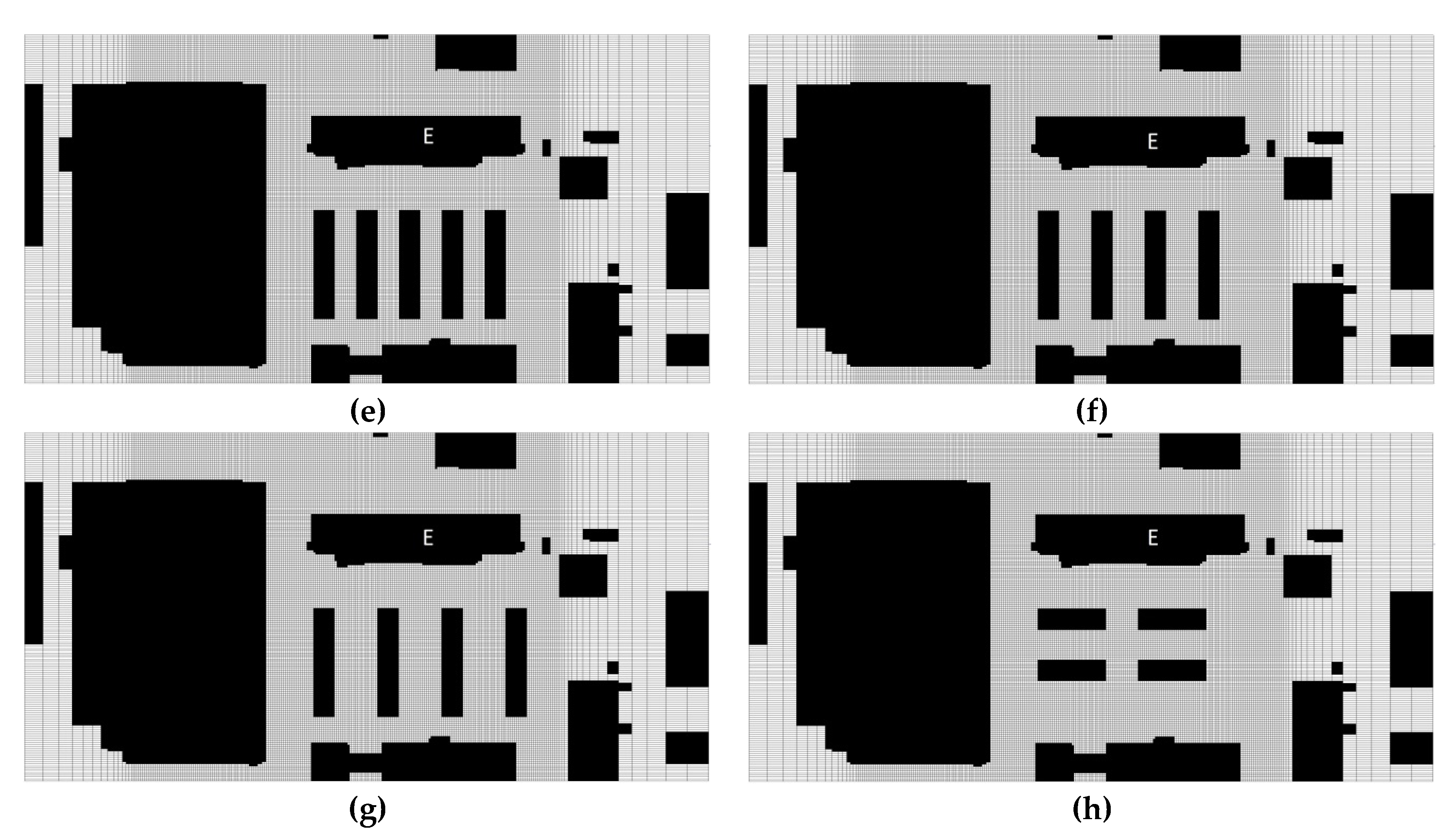
  • Scenario E: north-west to south-east oriented buildings with 19 m height;
  • Scenario F: buildings arranged at right angle to ENERGYbase (10 m distance between buildings);
  • Scenario G: buildings arranged at right angle to ENERGYbase (15 m distance between buildings);
  • Scenario H: buildings arranged at right angle to ENERGYbase (20 m distance between buildings);
  • Scenario I: buildings arranged in parallel to ENERGYbase with 24 m height;
  • Scenario J: buildings arranged in parallel to ENERGYbase, southerly buildings with 15 m height, northerly buildings with 19 m height.
The building configuration of the different scenarios is depicted in Figure 4a–h.

3. Results

3.1. Measured and Simulated Vertical Wind Profiles within the UCL

Vertical profiles of horizontal wind speed above roof top of the building ENERGYbase were simulated with the model MISKAM with an upper boundary condition of 10 m s−1 wind speed at 100 m AGL for the main wind directions 135°, 270° and 300°. The simulated profile of the horizontal wind speed within the lowest 30 m above the roof top at the model grid point situated at the center of the building is depicted as solid line in Figure 5. The model setup was described in Section 2.2. In the presented case, the flow simulation was conducted based on the building configuration of scenario A (Figure 4a). The model results were compared to temporarily averaged mast and SODAR measurements (Figure 5). Mast data with a temporal resolution of 10 min observed in the time-period December 2015 to November 2016 were filtered for the prevailing upper level wind conditions. This filtering was undertaken according to the wind speed and wind direction measured at the same time by the SODAR at 100 m AGL. For this purpose, all time-periods with bins with SODAR wind direction of 135°, 270° and 300° ±   5° and with SODAR wind speeds within ± 1 m s−1 were selected. The resulting filtered wind speeds from the one year of mast measurements and of SODAR data observed between 1 December 2015 and 30 November 2016 were averaged per observation height and depicted in Figure 5. In addition, a theoretical wind profile was computed according to equation 1 with a friction velocity set to the value 1.0 m s−1, z0 of 1.9 m and zd of 13.3 m (dashed line in Figure 5), where z0 and zd were derived from an average building height typical for the area of 19 m (Figure 2) multiplied by the empirical factors 0.1 and 0.7, respectively.
Under southeasterly flow conditions (135°), the mast measurements were on average in agreement with the theoretical wind profile (Figure 5a). The wind measurements at 6 m above roof at the two masts WM6m and WM10m were on average similar under these flow conditions. Furthermore, hardly any vertical variation was found from the mast measurements at 6 m, 9 m and 10 m above the roof. With southeasterly winds, the mast measurements were representing the flow conditions at the building center and close to the leeward side of the building (Figure 2). The mean SODAR wind speeds observed under these flow conditions revealed a slightly stronger increase of wind speed at 35 m AGL and 45 m AGL (comparable to 16 m and 26 m above roof top) than the theoretical profile. The MISKAM profile for this flow direction revealed an even more intense vertical gradient of wind speed. The modeled wind speed at 5 m above roof top underestimated the wind speeds observed at the masts under all three flow conditions, most in the case with 135° flow direction depicted in Figure 5a. The model simulated the formation of a recirculation zone above the building with wind speeds close to 1 ms−1 within the lowest model level above the obstacle while the mast measurements revealed that wind speeds of about 5 ms−1 were observed in this case. This could be optimized by reducing the roughness parameter used for roof surfaces in the model set-up to represent small scale structures of architecture that cannot be resolved explicitly. It would be necessary to test whether another choice of this parameter leads to better results in other cases, too.
Figure 5b,c revealed for westerly and northwesterly winds that the wind speeds at 6 m above roof top at WM6m, which is positioned 3 m from the western edge of the roof, were on average higher than the wind speeds observed at 6 m above roof in the center of the building (lower measurement value of WM10m). This indicates that the flow was accelerated at the edge of the roof in cases when WM6m was close to the luv-side of the building (Figure 5b,c). The flow separates from the edge of the roof and moves upwind. The negative pressure gradient on the roof due to the separation of the flow formed a cavity zone. Within this cavity region, wind speeds at 6 m above roof were about 1 ms-1 lower than at the edge (Figure 5c), comparable wind speeds were observed at 10 m height above roof (WM10m).
In situations with westerly upper level flow, the SODAR site obviously was less influenced by the next building structures leading to significantly higher wind speeds at 14 and 24 m above roof top compared to MISKAM and the theoretical profile. The modeled wind profile for this case was in very good agreement with the measurements at 9 m and 10 m above roof top as well as with the theoretical profile (Figure 5b).
The best agreement between measurements and model results was found for northwesterly flow conditions (Figure 5c). The mean SODAR wind speeds are about 0.5 ms−1 lower than the modeled values.

3.2. Impact of Changes in Adjacent Building Structures on Wind Conditions at Roof Top

In order to use the CFD model to quantify the impact of changes in building structure in the vicinity on the wind conditions at selected grid points above roof top, the fraction between wind speeds above roof top simulated for different scenarios was computed as factor F
F ( d 100 m ) = v z , s z e n a r i o   x ( d 100 m ) v z ,   s c e n a r i o   a ( d 100 m ) ,
with v the horizontal wind speed at height z simulated with MISKAM for a respective scenario (with x = A to J) and d100m representing the undisturbed flow direction at the upper boundary of the UCL (at 100 m AGL). The resulting fractions are listed in Table 1 and Table 2 for the five wind direction bins, which were observed most frequently in the area according to the SODAR measurements at 105 m above ground (Figure 3). It needs to be pointed out that the wind speed values were derived from the model output at the grid points representative for the mast sites WM6m and WM10m depicted in Figure 2 only. WM6m represents a position close to a corner of the building and at 6 m height above the roof. WM10m was situated more or less in the middle of the building at 10 m height above the roof. The results, as well as the further conclusions, were strongly dependent on the position of the considered grid points and could not be generalized.
The results revealed that depending on the flow direction at 100 m AGL, wind speeds above the roof top might increase or decrease when the building structures change in the vicinity of the site. It has to be kept in mind that the main motivation for this investigation was to find out, whether changes in building structure in the vicinity might have an impact on the energy yield of a roof-mounted small wind turbine. The theoretical energy output of a wind turbine was proportional to the third power of wind speed as, e.g., explained by [25]. Therefore, a slowdown of the flow to half of the wind speed for example would reduce the wind power to an eighth of the previous yield.
The model results indicate an increase of wind speeds of 2% at 6 m above roof top for scenario B (completed building) and J (buildings arranged in parallel to ENERGYbase with 15 m and 19 m building heights) in the case of east-south-easterly flow direction 120° (Table 1). All other simulated conditions result in a decrease of wind speed at this height, resulting in a decrease of maximum possible energy yield. The strongest decrease in wind speed at 6 m above roof top with 47% (proportional to a wind speed fraction factor of 0.53) was found in the model results for scenario D (north-west to south-east oriented buildings with 24 m height) in the case of south-south-easterly flow (150°). In this case, the roof top of the buildings at luv-side was at the same height as the selected grid point. Thus, the point of investigation was situated at the upper edge or within the cavity zone of the neighboring buildings.
Considering the operation of a small wind turbine at this site, these findings indicate that under the respective flow direction, 6% more wind power could be expected with scenario B and J, while the other scenarios led to a possible reduction of the energy yield to about a seventh of the energy yield (fraction factor of 0.533 = 0.15).
At 10 m above the roof top, the model simulations revealed that wind speeds were expected to be higher in all scenarios than in Scenario A (without building) for west-north-westerly flow (300°), which was the most frequent wind direction prevailing at the upper boundary of the UCL in the area (Table 2). The difference between the simulated wind speeds at 10 m above roof top reached 10–17% in the Scenarios D–H with buildings arranged in a rectangle to ENERGYbase or oriented northwest to southeast. All scenarios with buildings parallel to ENERGYbase led to a weaker increase of 2–6% at 10 m above the roof top. For all other wind directions, a decrease of wind speed compared to Scenario A was found. The strongest decrease of wind speed at 10 m above roof top was found for scenario D (north-west to south-east oriented buildings with 24 m height) and east-south-easterly flow (150°) with 23% (fraction factor 0.77). This is the same situation as described before for the maximum decrease of wind speed at 6 m above the roof top. Obviously, the deceleration of the flow by the 24 m high building situated luv-side in this case still had a significant impact on the wind speed at 10 m above the roof top (29 m AGL).
Again, these findings were interpreted in terms of relevance for small wind turbine operation at this site. Increasing the wind speed in this case with a factor of 1.17 results in an increase of wind power with a factor of 1.6. Whether this is relevant depends on the average wind speed and the total amount of energy yield. This was discussed further in the following based on the average wind speeds which were observed at the three sites.
As the SODAR measurements ended in November 2016 before the start of the construction activities next to the ENERGYbase building, no filtering of the observational data according to the upper level winds was possible for the conditions of Scenario B and C as presented in Section 3.1. The mean wind speeds averaged for the periods with no building at the adjacent property (Scenario A), with the finished closed building at this place (Scenario B) and during the construction period while the building shell resembled an open multi-store car park (Scenario C) were computed from the available measurements and compared to the undisturbed average 10 m AGL wind speed at the rural station in Table 3. It has to be kept in mind that the temporal averages cover different seasonal periods and years and are influenced by a variety of weather patterns. Nevertheless, it turns out that the results indicate that the wind speeds were up to 11% higher above roof top on average, than at 10 m AGL at the rural site with the car park situation nearby while the time periods with conditions of Scenario A and B revealed wind speed averages in the order or even below the mean 10 m AGL wind speed at the rural site.

4. Discussion

Vertical profiles of horizontal wind speed above the roof top of the building ENERGYbase were simulated with MISKAM for the main flow directions 135°, 270° and 300° and compared to temporarily averaged mast and SODAR measurements under comparable conditions. The model results were confirmed by the measurements at 9 m and 10 m above the roof top. On the other hand, the model obviously tended to simulate a stronger deceleration of the flow close to the roof than observed by the mast measurements. The differences in modeled and measured wind speeds within the cavity zone above the roof were found to be up to a maximum 20%, which was a significant underestimation of wind speed if used for site assessment for a wind turbine or if used for dispersion modeling of releases at roof level. The mean wind profile observed at the SODAR site was not fully representative for the conditions above the roof top and revealed a much stronger increase of wind speed with height under westerly flow conditions.
A model study was conducted with MISKAM for the different Scenarios A to J with varying building structures next to the site of investigation. The scenarios that were considered in the study represent typical structures, which could be found in the surroundings of the area of investigation. In case of the construction of single, very tall buildings, the impact on the surrounding wind field was expected to be much more significant. The model results revealed that the obstacles at the adjacent property might lead to an increase of wind speed above the roof top up to 17% or to a maximum decrease of up to 43% depending on the flow direction at the upper boundary of the UCL. Acceleration due to the changes in the building structure in this case turned out to be more effective at 10 m above roof top, while the deceleration effects were more visible at 6 m above roof top. The results deduced from measured time-series of wind speed above roof top and at the next rural station presented in Table 3 finally confirmed the findings from the model study that the changes in the building structure in the vicinity had an impact on the wind measurements above the roof top.
The measurement campaign was designed with focus on site assessment for small wind turbine (SWT) operation in urban environment. The measurements revealed that mean wind speeds of about 3–3.6 m s−1 were prevailing at this site (Table 3), which was considered as relatively low concerning the energy yield for the operation of a SWT [26]. Comparing the theoretical energy yield, the impact on the wind speed due to the change in building structure in Scenario B to J would have a negligible effect on the energy yield of the SWT in the order of only 1–3 W.
The changes in wind speed were found in the order of a maximum increase or decrease of 10% in this study. This turns out to be negligible concerning the energy yield of a roof-top small wind turbine due to the generally low prevailing wind speeds of about 3.5 m s−1. Nevertheless, wind speed changes of this order could be significant for wind energy yield in urban areas with higher mean wind speeds. This effect in any case needs to be considered in siting and conducting an urban meteorological monitoring network in order to ensure the homogeneity of observed time-series and may alter the emission and dispersion of pollutants or odor at roof level.

5. Conclusions

Following the recommendations given by WMO [1], wind measurements were conducted at 9 m and 10 m above the roof top corresponding to 1.5 times the mean building height. The model case study conducted with the CFD model MISKAM revealed that the wind speed at this height was affected by changes in building structure at an adjacent property. The impact might lead to an increase or decrease in the wind speed depending on the main flow direction, frequency of weather patterns leading to this flow direction and height and structure of the new buildings.
Wind measurements above the roof top were furthermore used as input for pollution dispersion modeling in urban areas, especially in the local scale. Alterations in the urban environment affected the wind conditions at the roof level and thus also might have implications on the release and dispersion of pollutants or odor in this height. The aspects of representativeness and homogeneity require consideration in the planning of new urban meteorological monitoring sites and in the operation of the meteorological network [. CFD modeling as presented in this study is useful to quantify the impact of building projects.

Author Contributions

Conceptualization, methodology and writing, K.B.-S. and S.S.; model study and visualization, F.F.; model setup and supervision of model study, G.R.; analysis of measurements, T.C. and K.B.-S.; revision supported by M.P. All authors have read and agreed to the published version of the manuscript.

Funding

This research was funded by Austrian Research Promotion Agency (FFG), grant number 845184 and by the Austrian Federal Ministry of Education, Science and Research.

Acknowledgments

The authors acknowledge Christoph Tiefgraber, Energiewerkstatt (Vereinsregister Nr. 569578895) for conduction of the mast measurements and provision of data and measurement reports.

Conflicts of Interest

The authors declare no conflict of interest. The funders had no role in the design of the study; in the collection, analyses, or interpretation of data; in the writing of the manuscript, or in the decision to publish the results.

References

  1. World Meteorological Organization. Initial Guidance to Obtain Representative Meteorological Observations at Urban Sites, Instruments and Observing Methods; Report No. 81, WMO/TD-No.1250; WMO: Geneva, Switzerland, 2006. [Google Scholar]
  2. Piringer, M.; Joffre, S. (Eds.) The Urban Surface Energy Budget and Mixing Height in EUROPEAN cities: Data, Models and Challenges for Urban Meteorology and Air Quality; Final Report of Working Group 2 of COST-715 Action; Demetra Ltd.: London, UK, 2005; 239p. [Google Scholar]
  3. Muller, C.; Chapman, L.; Grimmond, C.S.B.; Young, D.T.; Cai, X. Sensors and the City: A review of urban meteorological networks. Int. J. Climatol. 2013, 33, 1585–1600. [Google Scholar] [CrossRef]
  4. Rafailidis, S. Influence of Building Areal Density and Roof Shape on the Wind Characteristics Above a Town. Bound.-Layer Meteorol. 1997, 85, 255. [Google Scholar] [CrossRef]
  5. Britter, R.E.; Hanna, S.R. Flow and dispersion in urban areas. Annu. Rev. Fluid Mech. 2003, 35, 469–496. [Google Scholar] [CrossRef]
  6. Barlow, J.F. Progress in observing and modelling the urban boundary layer. Urban Clim. 2014, 10, 216–240. [Google Scholar] [CrossRef] [Green Version]
  7. Kastner-Klein, P.; Rotach, M. Mean flow and turbulence Characteristics in an urban roughness sublayer. Bound.-Layer Meteorol. 2004, 111, 55–84. [Google Scholar] [CrossRef]
  8. Grimmond, C.S.B.; Oke, T.R. Aerodynamic properties of urban areas derived from analysis of urban form. J. Appl. Meteorol. 1999, 38, 1262–1292. [Google Scholar] [CrossRef]
  9. Davenport, A.G.; Grimmond, C.S.B.; Oke, T.R.; Wieringa, J. Estimating the roughness of cities and sheltered country. In Proceedings of the 12th Conference on Applied Climatology, Asheville, NC, USA, 8–11 May 2000; American Meteorological Society: Boston, MA, USA, 2000; pp. 96–99. [Google Scholar]
  10. Fisher, B.; Joffre, S.; Kukkonen, J.; Piringer, M.; Rotach, M.; Schatzmann, M. (Eds.) Final Report COST Action 715; Demetra Ltd.: London, UK, 2005; pp. 27–46. [Google Scholar]
  11. Rotach, M.; Batchvarova, E.; Berkowicz, R.; Brechler, J.; Janour, Z.; Karjny, E.; Georgieva, E.; Middleton, D.; Osrodka, L.; Prior, V.; et al. Modification of flow and turbulence structure over urban areas. In Meteorology Applied to Urban Air Pollution Problems; Demetra Ltd.: Sofia, Bulgaria, 2005; pp. 27–46. ISBN 954-9526-30-5. [Google Scholar]
  12. Hanna, S.; White, J.; Zhou, Y. Observed winds, turbulence, and dispersion in built-up downtown areas of Oklahoma City and Manhattan. Bound.-Layer Meteorol. 2007, 125, 441–468. [Google Scholar] [CrossRef]
  13. Wood, C.R.; Arnold, S.J.; Balogun, A.A.; Barlow, J.F.; Belcher, S.E.; Britter, R.E.; Cheng, H.; Dobre, A.; Lingard, J.J.N.; Martin, D.; et al. Dispersion Experiments in Central London: The 2007 DAPPLE Project. Bull. Am. Meteorol. Soc. 2009, 90, 955–969. [Google Scholar] [CrossRef]
  14. Schatzmann, M.; Leitl, B. Validation and application of obstacle-resolving urban dispersion models. Atmos. Environ. 2002, 36, 4811–4821. [Google Scholar] [CrossRef]
  15. Hertwig, D.; Efthimiou, G.C.; Bartzis, J.G.; Leitl, B. CFD-RANS model validation of turbulent flow in a semi-idealized urban canopy. J. Wind Eng. Ind. Aerodyn. 2012, 111, 61–72. [Google Scholar] [CrossRef]
  16. Hanna, S.; White, J.; Trolier, J.; Vernot, R.; Brown, M.; Gowardhan, A.; Kaplan, H.; Alexander, Y.; Moussafir, J.; Wang, Y.; et al. Comparisons of JU2003 observations with four diagnostic urban wind flow and Lagrangian particle dispersion models. Atmos. Environ. 2011, 45, 4073–4081. [Google Scholar] [CrossRef]
  17. Arnold, S.J.; ApSimon, H.; Barlow, J.; Belcher, S.; Bell, M.; Boddy, J.W.; Britter, R.; Cheng, H.; Clark, R.; Colville, R.N.; et al. Introduction to the DAPPLE Air Pollution Project. Sci. Total Environ. 2004, 332, 139–153. [Google Scholar] [CrossRef] [PubMed]
  18. Dobre, A.; Arnold, S.J.; Smalley, R.J.; Boddy, J.W.D.; Barlow, J.F.; Tomlin, A.S.; Belcher, S.E. Flow field measurements in the proximity of an urban intersection in London, UK. Atmos. Environ. 2005, 39, 4647–4657. [Google Scholar] [CrossRef]
  19. Eichhorn, J.; Kniffka, A. The Numerical Flow Model MISKAM: State of Development and Evaluation of the Basic Version. Meteorol. Z. 2010, 19, 81–90. [Google Scholar] [CrossRef]
  20. Yee, E.; Biltoft, C.A. Concentration fluctuation measurements in a plume dispersing through a regular array of obstacles. Bound.-Layer Meteorol. 2004, 111, 363–415. [Google Scholar] [CrossRef]
  21. Eichhorn, J.; Balczo, M. Flow and dispersal simulations of the Mock Urban Setting Test. In Proceedings of the 12th International Conference on Harmonization within Atmospheric Dispersion Modelling for Regulatory Purposes (HARMO12), Cavtat, Croatia, 6–9 October 2008; pp. 67–72. [Google Scholar]
  22. Goricsán, I.; Balczó, M.; Czader, K.; Rákai, A.; Tonkó, C. Simulation of flow in an idealised city using various CFD codes. Int. J. Environ. Pollut. 2011, 44, 359. [Google Scholar] [CrossRef]
  23. Franke, J.; Hellsten, A.; Schlünzen, H.; Carissimo, B. The COST 732 Best Practice Guideline for CFD simulation of flows in the urban environment: A summary. Int. J. Environ. Pollut. 2011, 44, 419–427. [Google Scholar] [CrossRef]
  24. Britter, R.; Schatzmann, M. (Eds.) Model Evaluation Guidance and Protocol Document; COST Action 732 Quality Assurance and Improvemnet of Microscale Meteorological Models; COST Office: Brussels, Belgium, 2007; 27p, ISBN 3-00-018312-4. [Google Scholar]
  25. Sarkar, A.; Behera, D.K. Wind Turbine Blade Efficiency and Power Calculation with Electrical Analogy. Int. J. Sci. Res. Publ. 2012, 2, 1–5. [Google Scholar]
  26. Casini, M. Small Vertical Axis Wind Turbines for Energy Efficiency of Buildings. J. Clean Energy Technol. 2016, 4, 56–65. [Google Scholar] [CrossRef] [Green Version]
Figure 1. Map of Vienna (grey shading indicating topography, red and yellow lines for highways and main streets) with the location of the site ENERGYbase at the Viennese district Floridsdorf (red dot, see Figure 2 for details) and the next rural meteorological station Gross-Enzersdorf (green dot) (source: OpenStreetMap).
Atmosphere 11 00087 g001
Figure 2. Map of the site of the buildings ENERGYbase (Eb) and FUTUREbase (Fb) with position of masts with wind measurements at 6 m (WM 6 m, light blue dot), at 9 m (WM 9m, mid-blue dot) and at 6 m and 10 m (WM 10m, dark blue dot) height at roof top and of position of the SODAR site (green dot).
Atmosphere 11 00087 g002
Figure 3. Frequency distribution of wind speed and wind direction depicted as wind rose from one year of SODAR data measured at 105 m AGL (10 min averages observed from 01.07.2015 00 MEZ to 30.06.2016 23:50 MEZ).
Atmosphere 11 00087 g003
Figure 4. Detail of the MISKAM model domain (horizontal cross section at street level) with horizontal shape of the buildings (black structures, ENERGYbase is indicated by white E) for (a) scenario A, (b) scenario B, (c) scenario C, (d) scenario D and E, (e) scenario F, (f) scenario G, (g) scenario H and (h) scenarios I and J (see text for explanation). Length scale is depicted in Figure 4a.
Atmosphere 11 00087 g004aAtmosphere 11 00087 g004b
Figure 5. Vertical profiles of wind speed above roof top of the building ENERGYbase (19 m AGL) from mast and SODAR measurements, simulated with the model MISKAM for an upper boundary condition of 10 ms−1 wind speed at 100 m AGL and wind direction (a) 135°, (b) 270° and (c) 300° at 100 m AGL for the building configuration of scenario A (Figure 4a) and calculated using equation 1 (theoretical profile) with u* = 1.0 ms-1, z0 = 1.9 m and zd = 13.3 m.
Atmosphere 11 00087 g005
Table 1. Fraction of modeled wind speed at point WM 6m above roof top for scenarios B–J to wind speed in scenario A under different upper level flow directions (at 100 m AGL).
Scenario120°150°270°300°330°
A1.001.001.001.001.00
B1.020.950.970.920.93
C0.980.780.960.920.94
D0.800.530.990.950.94
E0.810.710.960.910.91
F0.780.921.000.970.97
G0.810.900.960.910.92
H0.740.900.950.910.92
I0.980.730.960.930.91
J1.020.940.970.910.93
Table 2. Fraction of modeled wind speed at point WM 10 m (Figure 2) above the roof top for scenarios B to J to wind speed in scenario A (see text for explanation) under different upper level flow directions (at 100 m AGL).
Scenario120°150°270°300°330°
A1.001.001.001.001.00
B0.990.920.941.030.94
C1.000.820.941.020.94
D0.940.771.011.170.92
E0.910.820.961.110.86
F0.950.660.981.140.91
G0.870.680.921.100.91
H0.810.750.921.110.90
I0.980.820.941.060.89
J1.000.970.951.030.90
Table 3. Fraction of mean wind speed measured at WM 6 m, WM 9 m and WM 10 m (Figure 2) for scenarios A, B and C (represented by averages in the selected periods) to the 10 m AGL wind speed observed at the rural station Gross-Enzersdorf.
Scenario AScenario BScenario C
December 2015–December 2016June 2017–October 2017January 2017–February 2017
Mean Wind Speed (m s−1)
6 m (WM6m)3.03.23.2
9 m (WM9m)3.23.43.4
10 m (WM10m)3.33.53.6
10 m AGL rural3.23.13.5
Fraction Factor
6 m WM6m)0.941.020.92
9 m (WM9m)0.991.080.96
10 m (WM10m)1.031.111.02

