Article

Fine-Scale Modeling of Individual Exposures to Ambient PM2.5, EC, NOx, and CO for the Coronary Artery Disease and Environmental Exposure (CADEE) Study

1
Center for Public Health and Environmental Assessment, U.S. Environmental Protection Agency, Research Triangle Park, NC 27711, USA
2
Institute for the Environment, University of North Carolina at Chapel Hill, Chapel Hill, NC 27517, USA
3
Oak Ridge Institute for Science and Education (ORISE), U.S. Environmental Protection Agency, Chapel Hill, NC 27514, USA
4
Oak Ridge Associated Universities (ORAU), U.S. Environmental Protection Agency, Research Triangle Park, NC 27711, USA
5
Center for Measurements and Modeling, U.S. Environmental Protection Agency, Research Triangle Park, NC 27711, USA
6
Department of Medicine, Pulmonary and Critical Care Medicine, Durham VA Medical Center, Durham, NC 27705 USA
7
Center for Public Health and Environmental Assessment, U.S. Environmental Protection Agency, Chapel Hill, NC 27514, USA
*
Author to whom correspondence should be addressed.
Atmosphere 2020, 11(1), 65; https://doi.org/10.3390/atmos11010065
Submission received: 30 November 2019 / Revised: 23 December 2019 / Accepted: 31 December 2019 / Published: 3 January 2020
(This article belongs to the Special Issue Atmospheric Dispersion of Pollutants in Urban Environments)

Abstract

:
Air pollution epidemiological studies often use outdoor concentrations from central-site monitors as exposure surrogates, which can induce measurement error. The goal of this study was to improve exposure assessments of ambient fine particulate matter (PM2.5), elemental carbon (EC), nitrogen oxides (NOx), and carbon monoxide (CO) for a repeated measurements study with 15 individuals with coronary artery disease in central North Carolina called the Coronary Artery Disease and Environmental Exposure (CADEE) study. We developed a fine-scale exposure modeling approach to determine five tiers of individual-level exposure metrics for PM2.5, EC, NOx, and CO using outdoor concentrations, on-road vehicle emissions, weather, home building characteristics, time-locations, and time-activities. We linked an urban-scale air quality model, residential air exchange rate model, building infiltration model, global positioning system (GPS)-based microenvironment model, and accelerometer-based inhaled ventilation model to determine residential outdoor concentrations (Cout_home, Tier 1), residential indoor concentrations (Cin_home, Tier 2), personal outdoor concentrations (Cout_personal, Tier 3), exposures (E, Tier 4), and inhaled doses (D, Tier 5). We applied the fine-scale exposure model to determine daily 24 h average PM2.5, EC, NOx, and CO exposure metrics (Tiers 1–5) for 720 participant-days across the 25 months of the CADEE study. Daily modeled metrics showed considerable temporal and home-to-home variability of Cout_home and Cin_home (Tiers 1–2) and person-to-person variability of Cout_personal, E, and D (Tiers 3–5). Our study demonstrates the ability to apply an urban-scale air quality model with an individual-level exposure model to determine multiple tiers of exposure metrics for an epidemiological study, in support of improving health risk assessments.

1. Introduction

Epidemiological studies have found associations between exposure to ambient (i.e., outdoor-generated) fine particulate matter (PM2.5, particulate matter ≤2.5µm in aerodynamic diameter) and its component elemental carbon (EC), nitrogen oxides (NOx), and carbon monoxide (CO) and indices of acute respiratory and cardiovascular morbidity and mortality [1,2,3,4]. Most of these studies used central-site measurements of these air pollutants as exposure surrogates due to cost and participant burden of using indoor or personal air pollution monitoring devices. While these exposure surrogates are designed for studies where central site monitor is representative for the entire study domain, they might have limitations in urban-scale studies where air pollution concentrations can be highly elevated near transportation sources such as highways, railroads, or airports. Specifically, these exposure surrogates do not account for (1) fine-scale spatial and temporal variability of on-road vehicle emissions and dispersion, (2) building-to-building and temporal variability of indoor infiltration (i.e., attenuation) of ambient air pollutants, (3) person-to-person and temporal variability of time spent in different indoor and outdoor locations, and (4) variability of respiratory inhalation (i.e., inhaled dose) from time spent at various physical activity levels. Differences between exposure surrogates, such as central-site measurements, and true exposures contribute to exposure measurement error. Depending on the epidemiological study design, these errors can add bias or uncertainty in health effect estimates [5,6]. The significance of this issue was highlighted in several reports by the National Research Council and National Academies of Sciences [7,8,9,10]. To address the recommendations of these reports, we developed the Exposure Model for Individuals (EMI), which can help reduce measurement error and improve health effect estimation [11,12,13,14,15]. This study describes the application of EMI for ambient PM2.5, EC, NOx, and CO in the Coronary Artery Disease and Environmental Exposure (CADEE) study [16].
The goal of the CADEE study is to examine ambient air pollutant exposures and cardiovascular and hematologic effects in adults with coronary artery disease living in central North Carolina (NC). Using ozone measurements from two fixed-site air monitors, significant associations were previously found between daily ambient ozone concentrations and various acute (maximum lag of 5 days) adverse effects: (1) altered endothelial function, (2) increased blood levels of inflammatory markers: neutrophils, monocytes, and interleukin-6, and (3) increased blood levels of factors attributed to fibrinolysis: tissue plasminogen factor and plasminogen activator inhibitor-1 [16]. In this study, we applied EMI for a subsequent epidemiological analysis to address the possible limitation of using outdoor air pollutant concentrations from fixed-site monitors as exposure surrogates in the CADEE study.
The EMI predicts multiple tiers of individual-level exposure metrics for actual participants in epidemiological studies using outdoor concentrations, questionnaires, weather, and time-activity information [11]. We previously developed and applied EMI for an epidemiological study called the Diabetes and the Environment Panel Study (DEPS) [11,12]. In the DEPS, we used a residential air exchange rate (AER) model, building infiltration model, and microenvironment-based exposure model to predict residential indoor concentrations and personal exposures for ambient PM2.5.
For the CADEE study, we extended EMI to develop a refined exposure modeling approach that includes six additional capabilities. First, the exposure model includes four pollutants (PM2.5, EC, NOx, and CO), whereas the DEPS included only PM2.5 [12]. Second, we used a previously developed urban-scale air quality model (AQM) to determine background, on-road, and total concentrations of each pollutant [17]. Third, we used a previously evaluated global positioning system (GPS)-based microenvironment (ME) classification model called MicroTrac to determine time-spent in different ME, whereas for the DEPS, we used time-location diary information [18]. Finally, an accelerometer-based ventilation model called VTrac was developed and applied to predict inhaled dose from physical activity information.
Before applying EMI for epidemiological studies with limited exposure data, we previously calibrated and evaluated EMI with extensive exposure data from field studies to reduce model uncertainty. We used measurement data from multiple field studies to evaluate the residential AER model, infiltration model, and GPS-based MicroTrac model [11,12,14,15,18]. Using a cross-validation, we compared individual predictions with 591 daily measurements from 31 homes and participants in central NC, which is the same location as the CADEE study. Median absolute differences were 20% (2.0 µg/m3) for home indoor concentrations and 20% (1.8 µg/m3) for personal exposures for ambient PM2.5 [11].
In this paper, we develop ambient PM2.5, EC, NOx, and CO exposure metrics for the CADEE study. We used outdoor concentrations and on-road vehicle emission factors as inputs for the AQM, and used housing characteristics, weather, time-locations from GPS loggers, and time-activities from accelerometers as inputs for EMI. We will first describe the CADEE study design, and then describe the AQM and EMI algorithms, and the development of multiple tiers of daily exposure metrics for each study participant.

2. Materials and Methods

2.1. The CADEE Study Design

The CADEE study was designed to examine the relationship between exposures to different air pollutants and various indices of acute cardiovascular and hematologic effects in a cohort of adults with coronary artery disease. A previous publication describes the study design and clinical measurements [16]. Briefly, the study included 15 non-smoking adult participants that had undergone a cardiac catheterization at Duke University Hospital and resided in central NC. Each participant visited the U.S. Environmental Protection Agency (EPA) Human Studies Facility (HSF) in Chapel Hill, NC at 08:00 (±1.5 h) for two consecutive weekdays for up to 10 weeks between May 2012 and April 2014. On the first day, the participant was outfitted with a hip-mounted accelerometer (model Actical; Respironics Inc., Murrysville, PA, USA) and provided a GPS data logger (model BT-Q1000XT; Qstartz International, Taipei, Taiwan), which they carried for the next 24 h. Various clinical measurements were collected at baseline and the following day to yield a total of 120 participant-days of data. Written informed consent was given by all participants prior to enrollment, and the study was approved by the Duke University Institutional Review Board, the University of North Carolina at Chapel Hill Institutional Review Board, and the EPA Human Protocols Office.
Input data for EMI were obtained from the participants for their home building characteristics, time-locations, and time-activities. Daily questionnaires were used to collect occupant behavior related to building operation, including indoor temperature, open windows and doors, and operating window fans. The GPS and accelerometer data loggers were used to collect continuous participant locations and physical activity intensities, respectively.
Before each 24 h deployment of the GPS data logger, the GPS memory was cleared using QTravel software (version 1.2; Qstartz International, Taipei, Taiwan) and the battery was fully charged. The GPS was programmed to sample every 5 s and to collect the date, time, position (latitude, longitude), speed, number of satellites used, and position dilution of precision (dimensionless value ≥ 1 that indicates accuracy of GPS position due to the satellite geometry) [18]. The sampled data were stored in the GPS memory during the 24 h sampling period, and then downloaded and stored in a text file for the MicroTrac model described below.
Before each 24 h deployment of the accelerometer data logger, the accelerometer memory was cleared using Actical software (version 3.0; Respironics Inc., Murrysville, PA, USA). The accelerometer was programmed for 1 s epochs and to collect the date, time, activity counts (value that indicates intensity of motion). The sampled data were stored in the accelerometer memory during the 24 h sampling period, and then downloaded and stored in a text file for the VTrac model described below.

2.2. Tiers of Modeled Exposure Metrics

We modeled five tiers of daily exposure metrics for ambient PM2.5, EC, NOx, and CO for 15 study participants and their homes (Figure 1). The five tiers, which have increasing levels of complexity and information needs, include: (Tier 1) home outdoor concentrations; (Tier 2) home indoor concentrations; (Tier 3) personal outdoor concentrations; (Tier 4) exposures; (Tier 5) inhaled doses. Each tier is separated into contributions from background, on-road emissions and total. For each participant, 24 h average (08:00 to 08:00) exposure metrics were modeled on the days with clinical measurements, and on the five days before clinical visits to yield a total of 720 participant-days. The modeling and subsequent analysis were implemented using MATLAB software (version R2015a, Mathworks, Natick, MA, USA).

2.2.1. Home Outdoor Concentrations (Tier 1)

For Tier 1, hourly outdoor concentrations for PM2.5, EC, NOx, and CO were modeled at all Census block centroids in three counties (Durham, Orange, Wake) in central NC using a previously described urban-scale AQM that combines the Research LINE source dispersion model (R-LINE) and Space-Time Ordinary Kriging (STOK) model [17,19,20]. We conducted model simulations to estimate concentrations from on-road vehicle emissions, concentrations from background, and total ambient concentrations. The AQM concentrations at each participant’s home were obtained from the Census block concentrations corresponding to the home location. The details of the method are described elsewhere [17].
Briefly, the R-LINE model was used to model the concentrations from on-road sources. The traffic emissions from road segments were treated as line sources and calculated using a combination of road network, traffic activity, and pollutant-specific emission factors from EPA’s Mobile Vehicular Emission Simulator (version 2010b) [21,22]. The emission factors are categorized by road type, vehicle type, vehicle speed, and ambient temperature, which are required to calculate the actual emission from a specific roadway. These data were collected from multiple sources including the Federal Highway Administration’s road network, National Weather Service’s hourly meteorological observations, and EPA’s National Emissions Inventories [23].
The STOK model was used to model the background concentrations from all sources except for on-road vehicle emission. Following the method developed by Arunachalam et al. [20], STOK was used to interpolate monitoring data from EPA’s Air Quality System to Census block centroids [24]. This technique assumes that the concentration value at each estimation point is a linear combination of nearby observational data. The linear combination, also known as kriging weight, is determined by minimizing the estimation variance while satisfying the unbiased constraint. The STOK technique is implemented with Bayesian Maximization Entropy library [25]. The background concentration was added to the modeled on-road contribution to determine the total ambient concentration.

2.2.2. Home Indoor Concentrations (Tier 2)

For Tier 2, hourly home indoor concentrations (Cin_home) for ambient PM2.5, EC, NOx, and CO were determined from home outdoor concentrations (Cout_home; Tier 1) with a dynamic mass-balance infiltration model described by
dCin_home/dt = AER P Cout_home − (AER + kr) Cout_home
where AER is the hourly air exchange rate (h−1), P is the penetration coefficient (dimensionless), and kr is the indoor removal rate (h−1) [11,14]. For PM2.5, P and kr were previously estimated from homes in the same region of NC as the CADEE study (P = 0.84, kr = 0.21 h−1) [11,12]. For EC, NOx, CO, P and kr were obtained from literature-reported values (P = 0.98, 1.00, 1.00; kr = 0.29, 0.5, 0 h−1, respectively) [26,27,28]. The 24 h average Cin_home was calculated by averaging the hourly Cin_home across 24 h.
The hourly AER for each participant’s home was determined from questionnaires and weather using the extended Lawrence Berkeley Laboratory model (LBLX) [11,12,14,15,17]. The AER model is mechanistic by accounting for the physical driving forces of the airflows (i.e., pressure difference across building envelope from indoor-outdoor temperature differences, called the stack effect, and from wind). The LBLX model includes leakage airflow through unintentional openings in a building envelope (e.g., cracks around windows, doors), natural ventilation through controlled openings in the building envelope (e.g., open windows, doors), and mechanical ventilation from window fans.
The LBLX model was previously described and evaluated for homes in the same region of NC as the CADEE study [11,12,14]. Briefly, the leakage airflow is defined as
Qleak = Aleak (ks|TinTout| + kwU2)0.5
where Aleak is the effective air leakage area, ks is the stack coefficient, kw is the wind coefficient, Tin and Tout are the average indoor and outdoor temperatures, respectively, and U is the average wind speed (see Supplementary Materials).
The LBLX model accounts for natural ventilation airflow on days with open windows or doors, and mechanical ventilation airflow on days with window fans operating [11,12,13,14,15,29]. The days with open windows or doors, and windows fans operating were determined from the questionnaires collected on the days with clinical measurements. If a participant reported open windows, doors; or use of window fans, we assumed open windows, doors; or window fans, respectively, for the five days before questionnaires were collected (lag days for the subsequent health outcome analysis). The total airflow from leakage, natural ventilation, and mechanical ventilation is defined as
Qtotal = (Q2mech + Q2leak + Q2nat)0.5
where Qnat is the natural ventilation airflow through open windows or doors and Qmech is the mechanical ventilation airflow through window fans (see Supplementary Materials). The AER is calculated as Qtotal divided by building volume V.

2.2.3. Personal Outdoor Concentrations (Tier 3)

For Tier 3, personal outdoor concentrations (Cout_personal) at each 5 s interval for ambient PM2.5, EC, NOx, and CO were determined using a GPS-based outdoor concentration tracker (OCTrac) method. The OCTrac integrates the urban-scale AQM data with personal GPS data. The Cout_personal were determined by temporally and spatially matching the GPS data with the fine-scale outdoor concentrations. Each 5 s GPS sample was time-matched to the corresponding 1-h outdoor concentration map of the three NC counties. Then, the outdoor concentration for each GPS geolocation (latitude, longitude) was obtained from the closest Census block centroid. OCTrac accounts for missing GPS data (e.g., when entering steel-framed buildings) by using geolocation of previous GPS sample. For the five days before GPS data were collected (lag days), the participant’s geolocations were set to the same locations as the day with GPS data. For lag days on weekends, we replaced any GPS samples obtained on weekdays at their work geolocation with their home geolocation. The 24 h average Cout_personal was calculated by averaging the 5 s Cout_personal across 24 h.

2.2.4. Exposures (Tier 4)

For Tier 4, we determined exposures (E) at each 5 s interval for ambient PM2.5, EC, NOx, and CO as defined by
E = MEin_home Cin_home + [(MEin_work + MEin_other) Finf_other_bldg + MEin_vehicle Finf_vehicle + MEout] Cout_personal
where Finf_other_bldg and Finf_vehicle are the infiltration factors (dimensionless) for buildings other than homes and for vehicles, respectively. For PM2.5, EC, NOx, and CO, we set Finf_other_bldg and Finf_vehicle to literature-reported values (Finf_other_bldg = 0.64, 0.59, 1.00, 1.00; Finf_vehicle = 0.44, 0.44, 0.80, 1.00, respectively) [28,30,31]. The MEin_home, MEin_work, MEin_other, MEin_vehicle, MEout are binary indicator variables (dimensionless) for the participant’s microenvironment (ME) at each 5 s interval, which correspond to the five MEs (indoors at home, work, other; inside vehicles; and outdoors, respectively). To simplify Equation (4), we combined the three MEs associated with outdoors (outdoors at home, work, other) into one ME (outdoors). For the five days before GPS data were collected (lag days), the participant’s ME was set to the same values as the day with GPS data. For lag days on weekends, we replaced any MEin_work = 1 with MEin_home = 1. The 24 h average E were calculated by averaging the 5 s E across 24 h.
The participant’s ME at each 5 s interval was determined using the MicroTrac model, which was previously described and evaluated for participants living in the same region of NC as the CADEE study [18]. Briefly, MicroTrac is a classification model that uses GPS data and geocoded building boundaries to determine the participant’s ME. The MicroTrac determines which one of the seven MEs (indoors and outdoors at home, work, other; inside vehicles) corresponds to the participant’s location at each 5 s GPS sampling interval. In a previous study, MicroTrac estimates were compared with 24 h diary data from nine participants in central NC. MicroTrac correctly classified the ME for 99.5% of the daily time spent by the participants [18].

2.2.5. Inhaled Doses (Tier 5)

For Tier 5, we determined inhaled doses at each 5 s interval for ambient PM2.5, EC, NOx, and CO as defined by
Di = Ei MV AT/BSA
where Di (µg/m2 body surface area) is the inhaled dose (mass; µg) normalized by the participant’s body surface area (m2) in ME i, where i = 1, 2, 3, 4, 5, 6, 7 corresponding to indoors at home, work, other; inside vehicles; outdoors at home, work, other, respectively. The Ei is the 5 s exposure (µg/m3) from each ME i, MV is the 5 s inhaled ventilation rate (m3/min), AT is the timestep (min) that is set to 0.083 min (5 s), and BSA is the participant’s body surface area (m2). The 24 h accumulated dose in each ME was calculated by adding the 5 s doses across 24 h. The total 24 h accumulated dose was calculated by adding the 24 h accumulated dose in each ME.
The 5 s exposures from each ME are defined as
E1 = MEin_home Cin_home
E2 = MEin_work Finf_other_bldg Cout_pers
E3 = MEin_other Finf_other_bldg Cout_pers
E4 = MEin_vehicle Finf_vehicle Cout_pers
E5 = MEout_home Cout_pers
E6 = MEout_work Cout_pers
E7 = MEout_other Cout_pers
where Ei is the exposure from each ME i, where i = 1, 2, 3, 4, 5, 6, 7 corresponding to the following microenvironments: indoors at home; indoors at work; other indoors; inside vehicles; outdoors at home; outdoors at work; other outdoors.
To determine the participant’s MV at each 5 s interval, we developed the VTrac model. First, VTrac uses accelerometer data and the GPS-based MicroTrac model, as described above, to determine which one out of four physical activity intensity levels (PAL; sedentary, light, moderate, vigorous) corresponds to the participant’s activity level. At each 5 s interval, we added the 1 s accelerometer activity counts across the past 60 s (cpm; counts/min), and set the corresponding PAL based on literature-reported thresholds (sedentary: cpm < 100, light: 100 ≤ cpm < 1535, moderate: 1535 ≤ cpm < 3962, vigorous: cpm ≥ 3962) [32]. These reported PAL thresholds were determined specifically for the Actical accelerometer used in the CADEE study and were based on metabolic equivalent (METS) thresholds (sedentary: METS < 2.0, light: 2.0 ≤ METS < 3.0, moderate: 3.0 ≤ METS < 6.0, vigorous: METS ≥ 6.0). For the five days before accelerometer data were collected (lag days), the participant’s activity counts were set to the same values as the day with accelerometer data.
To account for possible misclassifications when the participant is inside vehicles, we used the MEs determined from the GPS-based MicroTrac. We set the PAL to sedentary when the time-matched ME is classified as inside vehicles, since the accelerometer may detect motion from the vehicles even though the participant is sitting (i.e., sedentary) inside a vehicle.
The VTrac model then determines age- and sex-specific MV for each PAL based on literature-reported normalized minute ventilation (NMV) (L/min/kg body weight) [33]. The NMV were determined from oxygen consumption rates and basal metabolic rates based on data from the National Health and Nutrition Examination Survey and EPA’s Consolidated Human Activity Database. The NMV were reported for: (1) each of the four PAL based on METS thresholds (sedentary: METS ≤ 1.5, light: 1.5 < METS ≤ 3.0, moderate: 3.0 < METS ≤ 6.0, vigorous: METS > 6.0), (2) 14 separate age categories, (3) both males and females. For the CADEE study, we used the reported median NMV for each PAL based on the participant’s age and sex. The MV is calculated as NMV multiplied by the participant’s body weight (kg).
The BSA is defined as
BSA = 0.007184 BH0.725 BW0.425
where BH is body height (cm) and BW is body weight (kg) [34].

3. Results

To apply the fine-scale exposure model for the CADEE study, we modeled five tiers of daily exposure metrics for all 15 study participants and their homes. Modeled concentrations of PM2.5, EC, NOx, and CO for daily 24 h averages (08:00–08:00) are provided, which are time-matched to the daily health measurements for a future epidemiological analysis. We modeled a total of 720 participant-days.
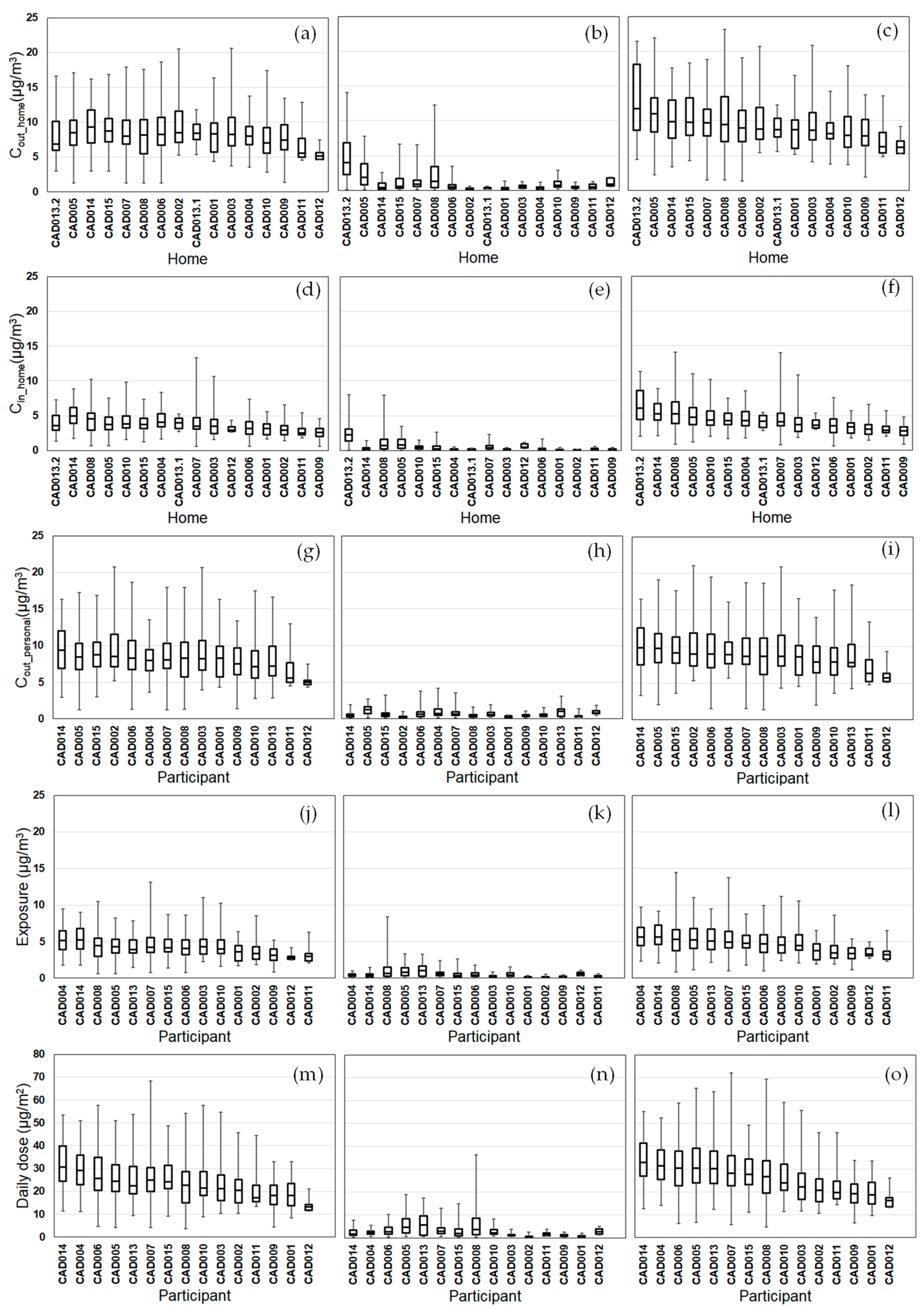
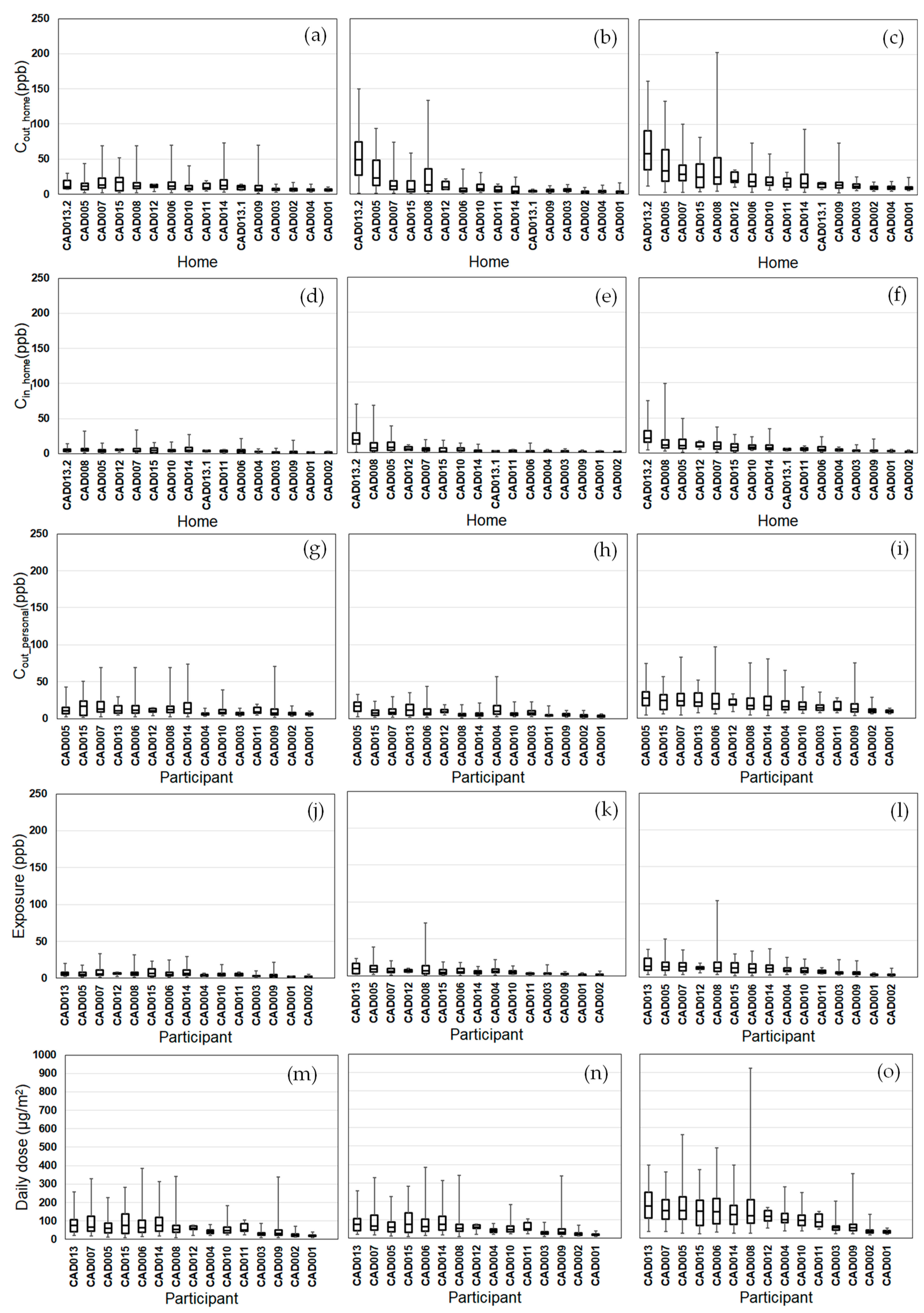
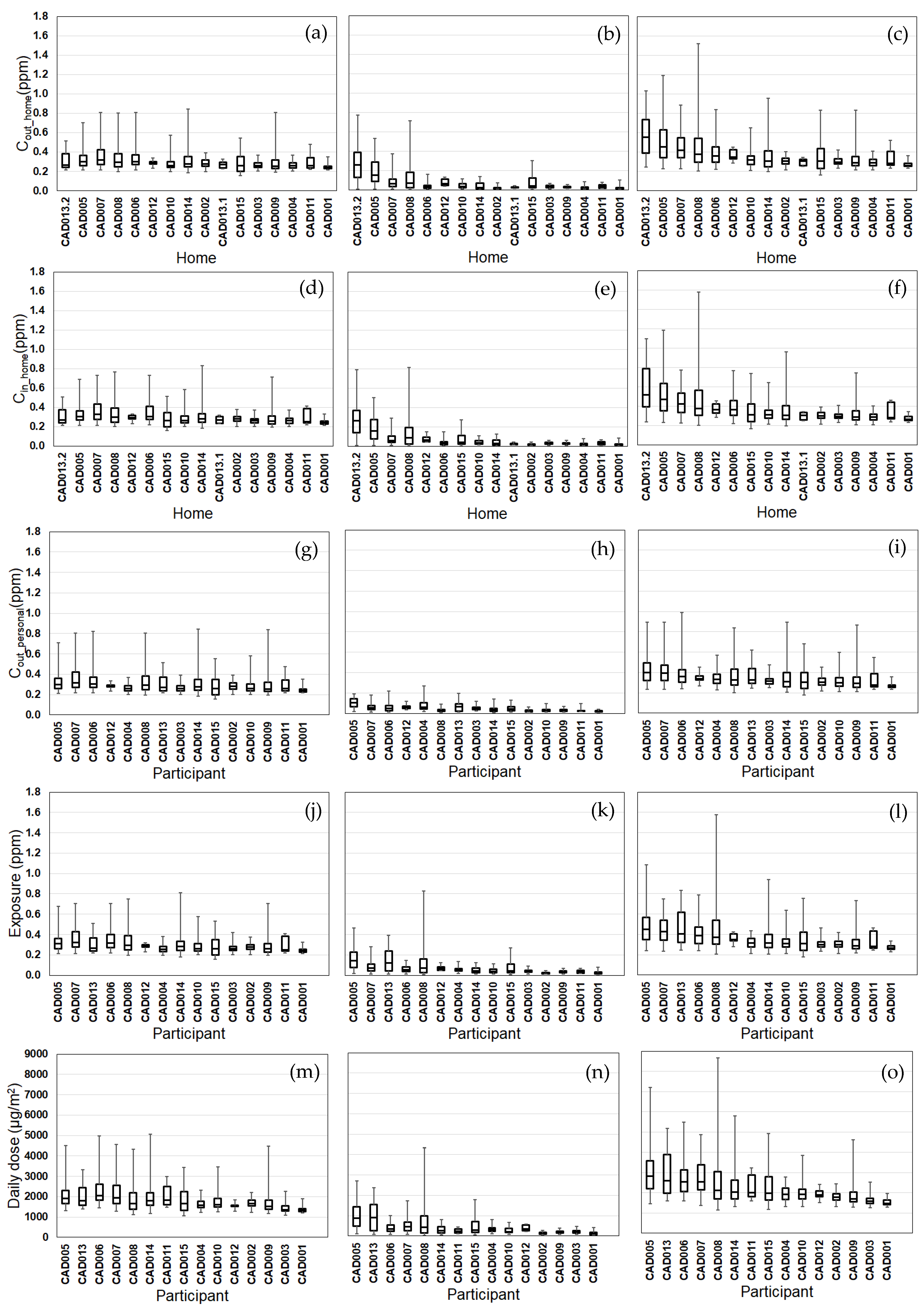
We compared the daily variability of the modeled exposure metrics for individual homes (Tiers 1–2) and participants (Tiers 3–5) (Figure 2, Figure 3, Figure 4 and Figure 5). For Tier 1, the temporal variability (within homes) and home-to-home variability of Cout_home was substantial for all four pollutants due to daily variations. Also, the on-road contribution to total Cout_home was larger than the background contribution for EC and NOx, and smaller for PM2.5 and CO due to substantial on-road emissions and near-road spatial gradients of EC and NOx.
For Tier 2, Cin_home was substantially lower than Cout_home for PM2.5, EC, and NOx, but the same for CO due to the home indoor attenuation of ambient PM2.5, EC, and NOx, but no indoor attenuation of CO. In the plots of the homes ranked by median Cin_home and Cout_home, the order of the homes for Cin_home was different than Cout_home for PM2.5, EC, and NOx due to the temporal and home-to-home variability of the residential AER from indoor-outdoor temperature differences, wind speed, and building operating conditions (e.g., open windows). The home-to-home variability was also due to building leakage area differences.
For Tier 3, Cout_personal was substantially different than Cout_home for EC, NOx, and CO, but similar for PM2.5 is due to the larger spatial variability of EC, NOx, and CO as compared to PM2.5. Also, the participant-to-participant variability between Cout_personal and Cout_home is due to time-of-day and duration at geolocations other than home.
For Tier 4, E was substantially lower than Cout_home for PM2.5, EC, and NOx, but the same for CO due to the indoor attenuation of ambient PM2.5, EC, and NOx, but no indoor attenuation of CO. In the plots of the participants ranked by median E and Cout_home, the order of the participants for E was different than Cout_home for PM2.5, EC, and NOx due to the temporal and participant-to-participant variability of time spent outdoors and within indoor microenvironments other than home and with different infiltration factors.
For Tier 5, the background contribution to total D was larger than the on-road contribution for PM2.5 and CO, smaller for EC, and similar for NOx. Also, the participants with high, moderate, and low median doses tended to be similar participants for EC, CO, and NOx, but not for PM2.5.
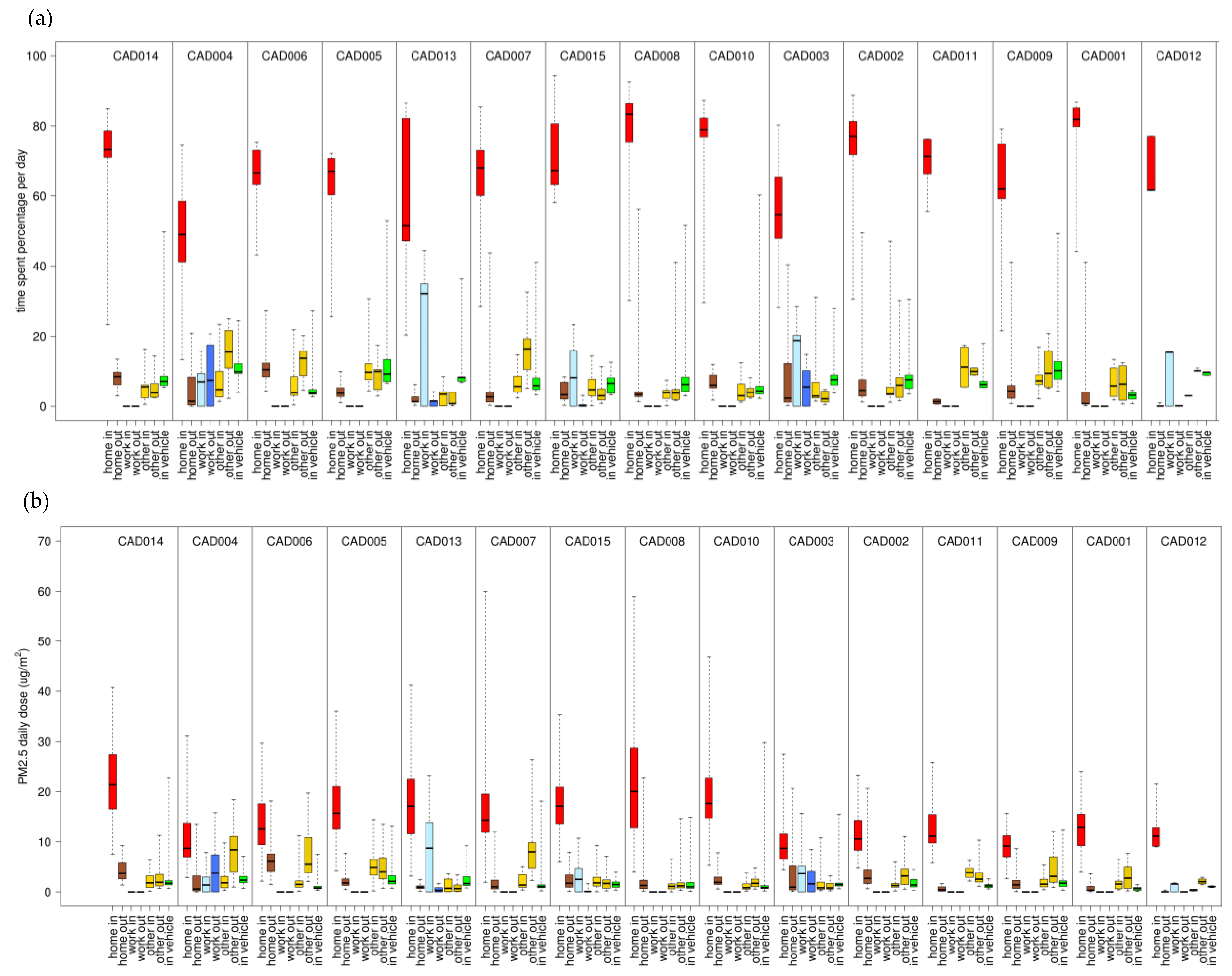
We compared the variability of daily D and time spent in each ME (Figure 6 and Figures S1–S4). For all participants, the highest median dose and greatest time spent was indoors at home. For the other six MEs, the ME with greater time spent usually corresponded to higher median dose for most participants. For CO, this was always the case. For PM2.5, EC, and NOx and for a few participants, the three indoor MEs (work, other, in-vehicles) with greater time spent corresponded to lower median doses as compared to the three outdoor MEs (home, work, other). This is likely due to the indoor and in-vehicle attenuation of ambient PM2.5, EC, and NOx, whereas ambient CO has no indoor or in-vehicle attenuation [26,27,28]. Also, the daily physical activity levels had substantial temporal and participant-to-participant variability for daily time spent performing at low intensity levels (e.g., walking) with an overall range of 20–390 min/day (Figure S5).

4. Discussion

Our goal was to determine daily ambient PM2.5, EC, NOx, and CO exposure metrics for each CADEE study participant in support of improving health effect estimation for future epidemiological analysis. Using a fine-scale exposure model, we performed an individual-level exposure assessment in the CADEE study that accounts for daily variations in ambient PM2.5, EC, NOx, and CO exposures separated by background, on-road vehicle emissions, and total concentrations based on an urban-scale AQM, a mechanistic house-specific AER model linked to a mass-balance infiltration model, infiltration factors for nonresidential buildings and vehicles, GPS-based microenvironment model, and accelerometer-based inhaled ventilation model. The impact of applying our fine-scale exposure model for an epidemiological study to improve health effect estimation will depend on various factors such as the health study design and the true exposure distributions [35,36]. We predicted multiple tiers of exposure metrics with different levels of complexity and uncertainty, which will be used in the epidemiological analysis to help determine the benefit of more sophisticated exposure metrics.
There are several benefits of using EMI for panel studies, such as the CADEE study, with individual-level health outcomes. First, spatio-temporal exposure models are needed that account for time-location variability of individuals that transition between microenvironments with different ambient pollutant concentrations. The National Research Council report: “Exposure Science in the 21st Century” highlighted the need for spatio-temporal exposure models that use input data for time-locations, housing characteristics, and ambient concentrations [7]. Second, population-level exposure models (e.g., Stochastic Human Exposure and Dose Simulation (SHEDS), Air Pollutants Exposure (APEX) models) predict exposures for demographic groups using population-level inputs from other studies, such as the U.S. Census [30,37,38]; whereas EMI predicts exposures for specific individuals in an epidemiological study using individual-level input data (e.g., questionnaires, time-location diaries) from each study participant. Thus, population exposure models are appropriate for studies with number of health outcomes across a region. The EMI is appropriate for panel studies, including studies that use personalized exposure, and genetic and cellular data to determine the role of individual susceptibility and effect modifiers on adverse responses to the four air pollutants [39]. The need for exposure models that are specific to susceptible individuals, such as people with cardiovascular and pulmonary disease, was highlighted in the National Research Council report on exposure science [7].
For exposure models, there are two types of measurement errors that can impact health effect estimates [6,35]. Berkson-like errors are from using a model that is missing some sources of variation or exposure factors. Classical-like errors are from uncertainty in the estimated model parameters. These errors can bias health effect estimates and alter confidence levels. Using our exposure modeling approach can minimize both types of errors. The urban-scale AQM can reduce Berkson-like error by accounting for spatio-temporal variability of outdoor concentrations. Our mechanistic AER model can reduce Berkson-like error by accounting for the home-to-home variations due to building characteristics and operation (e.g., window opening) and the temporal variations due to stack and wind effects [11,14]. The GPS-based MicroTrac model can also reduce Berkson-like error by accounting for the daily participant-to-participant variations in the time spent in various microenvironments with different infiltration factors [18]. Classical-like error can be reduced with our previous PM2.5 model calibration and evaluation to improve the estimated parameters of the mass balance residential infiltration model [11,12,14], and our previous evaluation of the MicroTrac model [18].
Variability in home infiltration of ambient air pollutants and subject time-location patterns that contribute to exposure variability can impact epidemiological studies [7]. Sarnat et al. accounted for the spatio-temporal variability of residential AER in Atlanta and found associations for the interaction between daily zip code-level AER and outdoor PM2.5, NOx, and CO concentrations on asthma emergency department visits [40]. Kaufman et al. accounted for temporal and house-to-house variability of PM2.5 infiltration and subject-specific time spent indoors for >6000 participants and found significant associations between individual-level ambient PM2.5 exposures and coronary artery calcification [41]. Koenig et al. also accounted for temporal and house-to-house variability of PM2.5 infiltration and daily time spent indoors for children with asthma and found ambient PM2.5 exposures were significantly associated with increases in exhaled nitric oxide [42]. These studies demonstrate the importance of accounting for individual-level exposure variability in epidemiological studies.
One limitation of this study is that the exposure metrics do not include non-ambient air pollutants. Wilson et al. showed the importance of separating ambient and non-ambient pollutant exposures since the EPA regulates only ambient pollutants, and pollutants from ambient and non-ambient sources have different chemical properties (particulate matter only) and temporal patterns, which can induce different health effects [43]. When we apply these modeled exposure metrics for epidemiological analysis, we plan to separately examine factors associated with non-ambient sources (e.g., gas stoves, environmental tobacco smoke) as categorical variables in the epidemiological models, which can remove potential uncertainties in modeled exposures that include indoor sources.
Another potential limitation of this study is that the exposure model uses outdoor air pollutant concentrations from a sophisticated urban-scale air quality model that requires substantial expertise and resources. For air pollutants that are spatially homogeneous (e.g., PM2.5), using fixed-site monitor measurements as inputs for the exposure model may be sufficient in certain geographical regions, except near large sources that can produce substantial spatial variations. In a previous study in central NC, we found no substantial difference between daily ambient PM2.5 exposures determined from a fixed-site PM2.5 monitors and those predicted from PM2.5 monitors outside each participant’s home [11]. For other air pollutants that can have substantial local spatial and temporal variations from nearby sources such as traffic (e.g., EC, NOx, CO), a fine-scale air quality model can account for this spatio-temporal variability. To facilitate and expand the use of exposure models for epidemiological studies, we developed a smartphone-based exposure model, called TracMyAir that determines individual-level exposure metrics for ambient PM2.5 and ozone [13]. The TracMyAir uses the smartphone’s geolocations to obtain real-time input data from the nearest outdoor air monitors. We plan to expand TracMyAir to automatically input data from urban-scale air quality models for other air pollutants with spatio-temporal variability.
Another potential limitation is that for the five lags days before GPS data were collected, the participant’s ME was set to the same values as the day with GPS data. For lag days on weekdays, we expect only small changes in daily time spent in different MEs since the GPS data was also collected on weekdays. For lag days on weekends, we replaced any time spent indoors at work with time spent indoors at home. To further examine how changes in the time spent in various MEs affect the resulting exposure, we performed a sensitivity analysis. The details of the method are described in Supplementary Materials. The sensitivity analysis showed that large changes in the time spent in MEs with substantially different infiltrations (e.g., indoors versus outdoors) can produce large changes in the exposures for PM2.5, EC, NOx, but have little or no effect on exposures to CO since infiltrations are similar for all ME. In this study, we expect small differences in the time spent in MEs on the lag days versus the day with GPS data. To reduce this potential exposure uncertainty, we developed a smartphone application for our exposure model called TracMyAir that will be used in future epidemiological studies to facilitate the collection of daily long-term time-location data [13].

5. Conclusions

This study demonstrates the ability of applying a fine-scale exposure model to determine five tiers of individual-level exposure metrics for the homes and participants in an epidemiological study. To improve exposure assessments in the CADEE study, EMI accounts for (1) hourly Census block outdoor concentrations for four ambient pollutants, (2) hourly house-specific infiltrations, (3) continuous (5-s) participant-specific time locations for seven MEs (indoors and outdoors at home, work, other; inside vehicles), and (4) continuous participant-specific inhaled ventilations. This capability can help improve exposure assessments for epidemiological studies, such as the CADEE study, in support of human health risk assessments.

Supplementary Materials

The following are available online at https://www.mdpi.com/2073-4433/11/1/65/s1. Figure S1: Percentage of time spent per day (%) (top) and daily dose (μg/m2) (bottom) of total Modeled PM2.5 for each microenvironment (home in, home out, work in, work out, other in, other out, in vehicle) for each participant, Figure S2: Percentage of time spent per day(%) (top) and daily dose (μg/m2) (bottom) of total Modeled EC for each microenvironment (home in, home out, work in, work out, other in, other out, in vehicle) for each participant, Figure S3: Percentage of time spent per day(%) (top) and daily dose (μg/m2) (bottom) of total Modeled CO for each microenvironment (home in, home out, work in, work out, other in, other out, in vehicle) for each participant, Figure S4: Percentage of time spent per day(%) (top) and daily dose (μg/m2) (bottom) of total Modeled NOx for each microenvironment (home in, home out, work in, work out, other in, other out, in vehicle) for each participant, Figure S5: Time spent per day (minutes) at different activity levels (light activity and all activities including light, moderate and vigorous) for each participant; Table S1: Stack coefficient ks ((L/s)2/(cm4 K)), Table S2: Wind coefficient kw ((L/s)2/(cm4 (m/s)2)), Table S3: Local sheltering, Table S4: Male sedentary ventilation rates (L/min/kg body weight), Table S5: Male light intensity ventilation rates (L/min/kg body weight), Table S6: Male moderate intensity ventilation rates (L/min/kg body weight), Table S7: Male vigorous intensity ventilation rates (L/min/kg body weight), Table S8: Female sedentary ventilation rates (L/min/kg body weight), Table S9: Female light intensity ventilation rates (L/min/kg body weight), Table S10: Female moderate intensity ventilation rates (L/min/kg body weight), Table S11: Female vigorous intensity ventilation rates (L/min/kg body weight).

Author Contributions

Conceptualization, M.B. (Michael Breen), V.I., and S.A.; methodology, M.B. (Michael Breen), M.S.C., M.B. (Miyuki Breen), Y.X., V.I., S.A., M.S.C., and R.D.; software, M.B. (Michael Breen), S.Y.C., and Y.X.; validation, M.B. (Michael Breen), S.Y.C., M.B. (Miyuki Breen), Y.X., V.I., S.A., M.S.C., and R.D.; formal analysis, M.B. (Michael Breen), S.Y.C., M.B. (Miyuki Breen), Y.X., V.I., S.A., M.C., and R.D.; investigation, M.B. (Michael Breen), S.Y.C., M.B. (Miyuki Breen), V.I., S.A., M.S.C., and R.D.; resources, M.B. (Michael Breen), V.I., S.A., M.S.C., and R.D.; data curation, M.B. (Michael Breen), S.Y.C., M.B. (Miyuki Breen), V.I., S.A., M.S.C., and R.D.; writing—original draft preparation, M.B. (Michael Breen); writing—review and editing, S.Y.C., M.B. (Miyuki Breen), Y.X., V.I., S.A., M.S.C., and R.D.; visualization, M.B., S.Y.C., M.B. (Miyuki Breen), and Y.X.; supervision, M.B. (Michael Breen), and S.A.; project administration, M.B. (Michael Breen), and S.A.; funding acquisition, M.B. (Michael Breen), V.I., M.S.C., and R.D. All authors have read and agreed to the published version of the manuscript.

Funding

This research received no external funding.

Acknowledgments

The authors thank David Heist for reviews and helpful suggestions. The views expressed in this article are those of the authors and do not necessarily represent the views or policies of the US Environmental Protection Agency. Mention of trade names or commercial products does not constitute endorsement or recommendation for use.

Conflicts of Interest

The authors declare no conflict of interest.

References

  1. U.S. EPA. Integrated Science Assessment (ISA) for Particulate Matter; Final Report 600/R-08/139F; U.S. EPA: Washington, DC, USA, 2009. Available online: https://cfpub.epa.gov/ncea/risk/recordisplay.cfm?deid=216546 (accessed on 25 November 2019).
  2. Janssen, N.; Joint, W.H. Health Effects of Black Carbon; Report for the Joint World Health Organization (WHO)/Convention Task Force on Health Effects of Air Pollution; WHO Regional Office for Europe: Copenhagen, Denmark, 2012; Available online: http://www.euro.who.int/en/publications/abstracts/health-effects-of-black-carbon-2012 (accessed on 25 November 2019).
  3. U.S. EPA. Integrated Science Assessment (ISA) for Oxides of Nitrogen—Health Criteria; Final Report 600/R-15/068; U.S. EPA: Washington, DC, USA, 2016. Available online: https://cfpub.epa.gov/ncea/isa/recordisplay.cfm?deid=310879 (accessed on 25 November 2019).
  4. U.S. EPA. Integrated Science Assessment (ISA) for Carbon Monoxide; Final Report 600/R-09/019F; U.S. EPA: Washington, DC, USA, 2010. Available online: https://cfpub.epa.gov/ncea/isa/recordisplay.cfm?deid=218686 (accessed on 25 November 2019).
  5. Zeger, S.L.; Thomas, D.; Dominici, F.; Sarnet, J.M.; Schwartz, J.; Dockery, D.; Cohen, A. Exposure measurement error in time-series studies of air pollution: Concepts and consequences. Environ. Health Perspect. 2000, 108, 419–426. [Google Scholar] [CrossRef] [PubMed]
  6. Sheppard, L.; Burnett, R.T.; Szpiro, A.A.; Kim, S.Y.; Jerrett, M.; Pope, C.A., III; Brunekreef, B. Confounding and exposure measurement error in air pollution epidemiology. Air Qual. Atmos. Health 2012, 5, 203–216. [Google Scholar] [CrossRef] [Green Version]
  7. National Research Council. Exposure Science in the 21st Century: A Vision and a Strategy; The National Academies Press: Washington, DC, USA, 2012. [Google Scholar] [CrossRef]
  8. National Research Council. Research Priorities for Airborne Particulate Matter: I. Immediate Priorities and a Long-Range Research Portfolio; The National Academies Press: Washington, DC, USA, 1998. [Google Scholar] [CrossRef]
  9. National Academies of Sciences, Engineering, and Medicine. Health Risks of Indoor Exposure to Particulate Matter: Workshop Summary; The National Academies Press: Washington, DC, USA, 2016. [Google Scholar] [CrossRef]
  10. National Academies of Sciences, Engineering, and Medicine. Using 21st Century Science to Improve Risk-Related Evaluations; The National Academies Press: Washington, DC, USA, 2017. [Google Scholar] [CrossRef]
  11. Breen, M.S.; Long, T.C.; Schultz, B.D.; Williams, R.W.; Richmond-Bryant, J.; Breen, M.; Langstaff, J.E.; Devlin, R.B.; Schneider, A.; Burke, J.M.; et al. Air Pollution Exposure Model for Individuals (EMI) in Health Studies: Evaluation for Ambient PM2.5 in Central North Carolina. Environ. Sci. Technol. 2015, 49, 14184–14194. [Google Scholar] [CrossRef] [PubMed] [Green Version]
  12. Breen, M.S.; Yadong, X.; Williams, R.; Schneider, A.; Devlin, R. Modeling Individual-level Exposures to Ambient PM2.5 for the Diabetes and the Environment Panel Study (DEPS). Sci. Total Environ. 2018, 626, 807–816. [Google Scholar] [CrossRef] [PubMed]
  13. Breen, M.S.; Seppanen, C.; Isakov, V.; Arunachalam, S.; Breen, M.; Samet, J.; Tong, H. Development of TracMyAir smartphone application for modeling exposures to ambient PM2.5 and ozone. Int. J. Environ. Res. Public Health 2019, 16, 3468. [Google Scholar] [CrossRef] [PubMed] [Green Version]
  14. Breen, M.S.; Breen, M.; Williams, R.W.; Schultz, B.D. Predicting residential air exchange rates from questionnaires and meteorology: Model evaluation in central North Carolina. Environ. Sci. Technol. 2010, 44, 9349–9356. [Google Scholar] [CrossRef]
  15. Breen, M.S.; Burke, J.M.; Batterman, S.A.; Vette, A.F.; Godwin, C.; Croghan, C.W.; Schultz, B.D.; Long, T.C. Modeling spatial and temporal variability of residential air exchange rates for the Near-Road Exposures and Effects of Urban Air Pollutants Study (NEXUS). Int. J. Environ. Res. Public Health 2014, 11, 11481–11504. [Google Scholar] [CrossRef] [Green Version]
  16. Mirowsky, J.; Carraway, M.; Dhingra, R.; Tong, H.; Neas, L.; Diaz-Sanchez, D.; Cascio, W.; Case, M.; Crooks, J.; Hauser, E.R.; et al. Ozone exposure is associated with acute changes in inflammation, fibrinolysis, and endothelial cell function in coronary artery disease patients. Environ. Health 2017, 16, 126. [Google Scholar] [CrossRef] [Green Version]
  17. Chang, S.Y.; Vizuete, W.; Valencia, A.; Naess, B.; Isakov, V.; Palma, T.; Breen, M.; Arunachalam, S. A modeling framework for characterizing near-road air pollutant concentration at community scales. Sci. Total Environ. 2015, 538, 905–921. [Google Scholar] [CrossRef]
  18. Breen, M.S.; Long, T.; Schultz, B.; Crooks, J.; Breen, M.; Langstaff, J.; Isaacs, K.; Tan, C.; Williams, R.; Cao, Y.; et al. GPS-based microenvironment tracker (MicroTrac) model to estimate time-location of individuals for air pollution exposure assessments: Model evaluation in central North Carolina. J. Exp. Sci. Environ. Epidemiol. 2014, 24, 412–420. [Google Scholar] [CrossRef]
  19. Snyder, M.G.; Venkatram, A.; Heist, D.K.; Perry, S.G.; Petersen, W.B.; Isakov, V. R-LINE: A Line Source Dispersion Model for Near-Surface Releases. Atmos. Environ. 2013, 77, 748–756. [Google Scholar] [CrossRef]
  20. Arunachalam, S.; Valencia, A.; Akita, Y.; Serre, M.L.; Omary, M.; Garcia, V.; Isakov, V. A method for estimating urban background concentrations in support of hybrid air pollution modeling for environmental health studies. Int. J. Environ. Res. Public Health 2014, 11, 10518–10536. [Google Scholar] [CrossRef] [Green Version]
  21. Cook, R.; Isakov, V.; Touma, J. Resolving local-scale emissions for modeling air quality near roadways. J. Air Waste Manag. Assoc. 2008, 58, 451–461. [Google Scholar] [CrossRef] [Green Version]
  22. Snyder, M.; Arunachalam, S.; Isakov, V.; Talgo, K.; Naess, B.; Valencia, A.; Omary, M.; Davis, N.; Cook, R.; Hanna, A. Creating Locally-Resolved Mobile-Source Emissions Inputs for Air Quality Modeling in Support of an Exposure Study in Detroit, Michigan. Int. J. Environ. Res. Public Health 2014, 11, 12739–12766. [Google Scholar] [CrossRef] [Green Version]
  23. U.S. EPA. 2011 National Emissions Inventory (NEI) Data. Available online: https://www.epa.gov/air-emissions-inventories/2011-national-emissions-inventory-nei-data (accessed on 25 November 2019).
  24. U.S. EPA. Air Quality System (AQS) User’s Guide. Available online: https://www.epa.gov/aqs/aqs-user-guide (accessed on 25 November 2019).
  25. Serre, M.L.; Christakos, G. Modern geostatistics: Computational BME analysis in the light of uncertain physical knowledge–the Equus Beds study. Stoch. Environ. Res. Risk Assess. 1999, 13, 1–26. [Google Scholar] [CrossRef]
  26. Meng, Q.Y.; Turpin, B.J.; Polidori, A.; Lee, J.H.; Weisel, C.; Morandi, M.; Colome, S.; Stock, T.; Winer, A.; Zhang, J. PM2.5 of ambient origin: Estimates and exposure errors relevant to PM epidemiology. Environ. Sci. Technol. 2005, 39, 5105–5112. [Google Scholar] [CrossRef] [Green Version]
  27. Weschler, C.J.; Shields, H.C.; Nalk, D.V. Indoor Chemistry Involving O-3, No, and No2 as Evidenced by 14 Months of Measurements at a Site in Southern California. Environ. Sci. Technol. 1994, 28, 2120–2132. [Google Scholar] [CrossRef] [PubMed]
  28. Dionisio, K.L.; Baxter, L.K.; Chang, H.H. An empirical assessment of exposure measurement error and effect attenuation in bipollutant epidemiologic models. Environ. Health Perspect. 2014, 122, 1216–1224. [Google Scholar] [CrossRef] [PubMed] [Green Version]
  29. Breen, M.S.; Schultz, B.; Sohn, M.; Long, T.; Langstaff, J.; Williams, R.; Isaacs, K.; Meng, Q.; Stallings, C.; Smith, L. A review of air exchange rate models for air pollution exposure assessments. J. Expo. Sci. Environ. Epidemiol. 2014, 24, 555–563. [Google Scholar] [CrossRef] [PubMed] [Green Version]
  30. Burke, J.M.; Zufall, M.J.; Ozkaynak, H. A population exposure model for particulate matter: Case study results for PM2.5 in Philadelphia, PA. J. Expo. Anal. Environ. Epidemiol. 2001, 11, 470–489. [Google Scholar] [CrossRef] [PubMed] [Green Version]
  31. Ott, W.; Klepeis, N.; Switzer, P. Air change rates of motor vehicles and in-vehicle pollutant concentrations from secondhand smoke. J. Expo. Anal. Environ. Epidemiol. 2008, 18, 312–325. [Google Scholar] [CrossRef] [PubMed]
  32. Colley, R.C.; Garriguet, D.; Janssen, I.; Craig, C.L.; Clarke, J.; Tremblay, M.S. Physical Activity of Canadian Adults: Accelerometer Results from the 2007 to 2009 Canadian Health Measures Survey; Report 82-003-XPE; Statistics Canada: Ottawa, ON, Canada, 2011; Available online: https://www150.statcan.gc.ca/n1/pub/82-003-x/2011001/article/11396-eng.pdf (accessed on 25 November 2019).
  33. U.S. EPA. Metabolically Derived Human Ventilation Rates: A Revised Approach Based upon Oxygen Consumption Rates; Final Report Report EPA/600/R-06/129F; U.S. EPA: Washington, DC, USA, 2009. Available online: https://cfpub.epa.gov/ncea/risk/recordisplay.cfm?deid=202543 (accessed on 25 November 2019).
  34. DuBois, D.; DuBois, E.F. A formula to estimate the approximate surface area if height and weight be known. Arch. Int. Med. 1916, 17, 863–871. [Google Scholar] [CrossRef] [Green Version]
  35. Szpiro, A.A.; Paciorek, C.J.; Sheppard, L. Does more accurate exposure prediction necessarily improve health effect estimates? Epidemiology 2011, 22, 680–685. [Google Scholar] [CrossRef] [PubMed] [Green Version]
  36. Szpiro, A.A.; Paciorek, C.J. Measurement error in two-stage analyses, with application to air pollution epidemiology. Environmetrics 2013, 24, 501–517. [Google Scholar] [CrossRef] [Green Version]
  37. U.S. EPA. Total Risk Integrated Methodology (TRIM) Air Pollutants Exposure Model Documentation (TRIM.Expo/APEX, Version 4.5); Report EPA/600/R-06/129F; EPA Office of Air Quality Planning and Standards: Research Triangle Park, NC, USA, 2012. Available online: https://www.epa.gov/fera/total-risk-integrated-methodology-trim-air-pollutants-exposure-model-documentation-trimexpo (accessed on 25 November 2019).
  38. U.S. EPA. Total Risk Integrated Methodology (TRIM) Air Pollutants Exposure Model Documentation (TRIM.Expo/APEX, Version 4.5) Volume II, Technical Support Document; Report EPA-452/B-12-001b; EPA Office of Air Quality Planning and Standards: Research Triangle Park, NC, USA, 2012. Available online: https://www.epa.gov/sites/production/files/2017-07/documents/apex45_usersguide_vol2_aug2012_0_1.pdf (accessed on 25 November 2019).
  39. Weis, B.K.; Balshaw, D.; Barr, J.R.; Brown, D.; Ellisman, M.; Lioy, P.; Omenn, G.; Potter, J.D.; Smith, M.T.; Sohn, L.; et al. Personalized exposure assessment: Promising approaches for human environmental health research. Environ. Health Perspect. 2005, 113, 840–848. [Google Scholar] [CrossRef] [Green Version]
  40. Sarnat, J.A.; Sarnat, S.E.; Flanders, W.D.; Chang, H.H.; Mulholland, J.; Baxter, L.; Isakov, V.; Özkaynak, H. Spatiotemporally resolved air exchange rate as a modifier of acute air pollution-related morbidity in Atlanta. J. Expo. Sci. Environ. Epidemiol. 2013, 23, 606–615. [Google Scholar] [CrossRef] [PubMed] [Green Version]
  41. Kaufman, J.D.; Adar, S.D.; Barr, R.G.; Budoff, M.; Burke, G.L.; Curl, C.L.; Daviglus, M.L.; Roux, A.V.; Gassett, A.J.; Jacobs, D.R., Jr.; et al. Association between air pollution and coronary artery calcification within six metropolitan areas in the USA (the Multi-Ethnic Study of Atherosclerosis and Air Pollution): A longitudinal cohort study. Lancet 2016, 388, 696–704. [Google Scholar] [CrossRef] [Green Version]
  42. Koenig, J.Q.; Mar, T.F.; Allen, R.W.; Jansen, K.; Lumley, T.; Sullivan, J.H.; Trenga, C.A.; Larson, T.; Liu, L.J. Pulmonary effects of indoor- and outdoor-generated particles in children with asthma. Environ. Health Perspect. 2005, 13, 499–503. [Google Scholar] [CrossRef] [Green Version]
  43. Wilson, W.; Mage, D.; Grant, L. Estimating separately personal exposure to ambient and nonambient particulate matter for epidemiology and risk assessment: Why and how. J. Air Waste Manag. Assoc. 2000, 50, 1167–1183. [Google Scholar] [CrossRef] [PubMed] [Green Version]
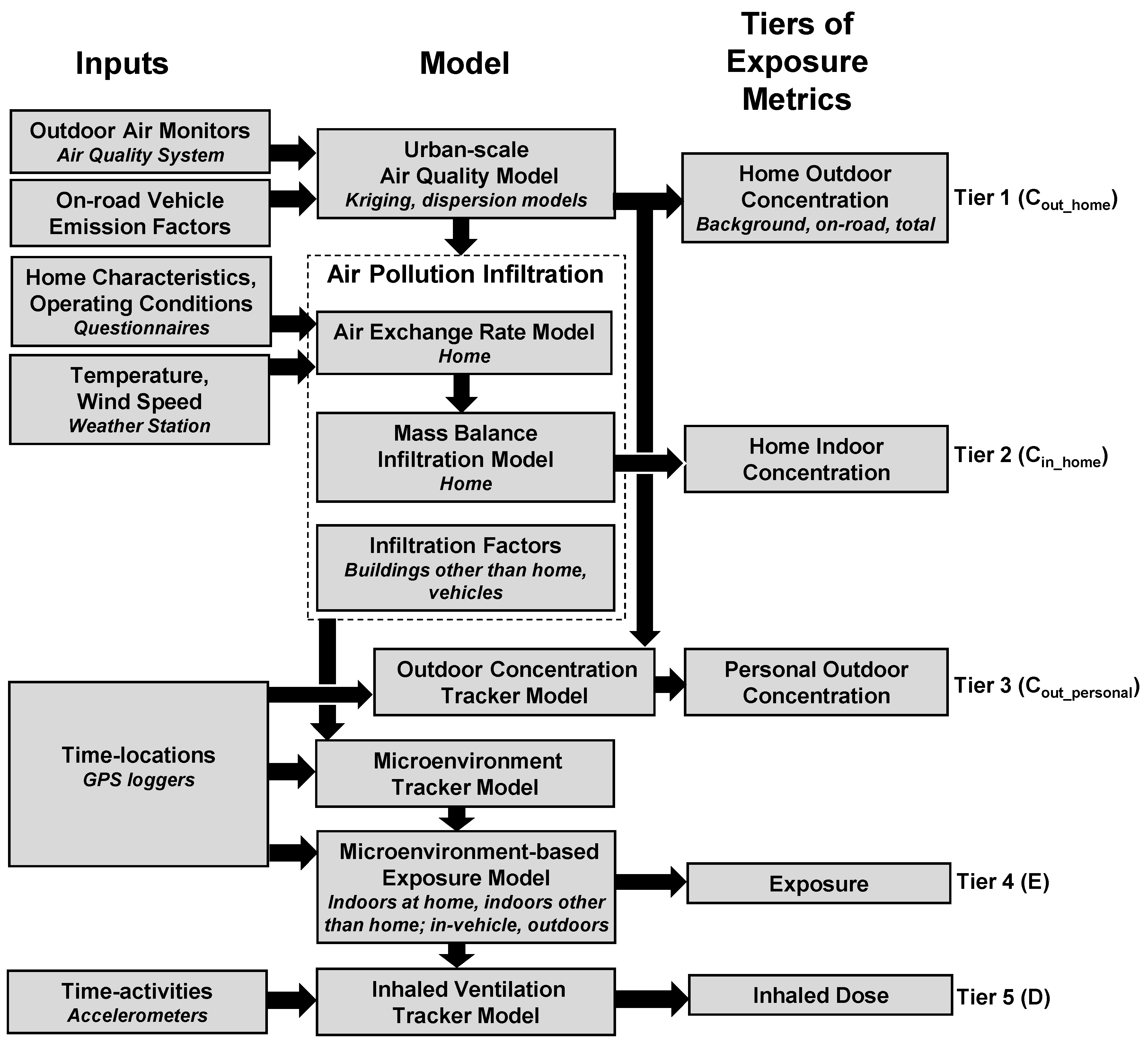
Figure 1. Conceptual model of Exposure Model for Individuals (EMI) to predict five tiers of individual-level exposure metrics for ambient fine particulate matter (PM2.5), elemental carbon (EC), nitrogen oxides (NOx), and carbon monoxide (CO). Tiers 1–2 (Cout_home—outdoor concentration; Cin_home—indoor concentration) are related to homes, and Tiers 3–5 (Cout_personal—personal outdoor concentration, E—exposure, D—inhaled dose) are related to participants.
Atmosphere 11 00065 g001
Figure 2. Modeled PM2.5 exposure metrics for Tier 1 (outdoor home concentrations; ac), Tier 2 (indoor home concentrations; df), Tier 3 (personal outdoor concentrations; gi), Tier 4 (exposures; jl), Tier 5 (inhaled dose; mo) from background (a,d,g,j,m), on-road vehicle emissions (b,e,h,k,n), and total PM2.5 (c,f,i,l,o). Results (24 h average, 08:00–08:00) are sorted by total PM2.5 median values from highest to lowest. Shown are medians with 25th and 75th percentiles, and whiskers for minimum and maximum values.
Atmosphere 11 00065 g002
Figure 3. Modeled EC exposure metrics for Tier 1 (outdoor home concentrations; a–c), Tier 2 (indoor home concentrations; df), Tier 3 (personal outdoor concentrations; gi), Tier 4 (exposures; jl), Tier 5 (inhaled dose; mo) from background (a,d,g,j,m), on-road vehicle emissions (b,e,h,k,n), and total EC (c,f,i,l,o). Results (24 h average, 08:00–08:00) are sorted by total EC median values from highest to lowest. Shown are medians with 25th and 75th percentiles, and whiskers for minimum and maximum values.
Atmosphere 11 00065 g003
Figure 4. Modeled NOx exposure metrics for Tier 1 (outdoor home concentrations; ac), Tier 2 (indoor home concentrations; df), Tier 3 (personal outdoor concentrations; gi), Tier 4 (exposures; jl), Tier 5 (inhaled dose; mo) from background (a,d,g,j,m), on-road vehicle emissions (b,e,h,k,n), and total NOx (c,f,i,l,o). Results (24 h average, 08:00–08:00) are sorted by total NOx median values from highest to lowest. Shown are medians with 25th and 75th percentiles, and whiskers for minimum and maximum values.
Atmosphere 11 00065 g004
Figure 5. Modeled CO exposure metrics for Tier 1 (outdoor home concentrations; ac), Tier 2 (indoor home concentrations; df), Tier 3 (personal outdoor concentrations; gi), Tier 4 (exposures; jl), Tier 5 (inhaled dose; mo) from background (a,d,g,j,m), on-road vehicle emissions (b,e,h,k,n), and total CO (c,f,i,l,o). Results (24 h average, 08:00–08:00) are sorted by total CO median values from highest to lowest. Shown are medians with 25th and 75th percentiles, and whiskers for minimum and maximum values.
Atmosphere 11 00065 g005
Figure 6. Percentage of daily time spent in (a) and inhaled dose for total PM2.5 (b) for each microenvironment (indoors and outdoors at home, work, and other; inside vehicle) and each participant. Results (24 h average, 08:00–08:00) are sorted by median values of the total dose from highest to lowest. Shown are medians with 25th and 75th percentiles, and whiskers for minimum and maximum values.
Atmosphere 11 00065 g006