Article

Seasonal Forecasting of the Onset of the Rainy Season in West Africa

1
Institute of Geography, University of Augsburg, 86159 Augsburg, Germany
2
Institute of Meteorology and Climate Research, Karlsruhe Institute of Technology, Campus Alpin, 82467 Garmisch-Partenkirchen, Germany
3
Competence Center, West African Science Service Centre on Climate Change and Adapted Land Use, Ouagadougou 9507, Burkina Faso
4
Training and Research Department, AGRHYMET Regional Centre, Niamey PB 11011, Niger
*
Author to whom correspondence should be addressed.
Atmosphere 2019, 10(9), 528; https://doi.org/10.3390/atmos10090528
Submission received: 31 July 2019 / Revised: 27 August 2019 / Accepted: 2 September 2019 / Published: 8 September 2019
(This article belongs to the Special Issue Improved (Sub)Seasonal Climate Forecast for Impact Modelling)

Abstract

:
Seasonal forecasts for monsoonal rainfall characteristics like the onset of the rainy seasons (ORS) are crucial for national weather services in semi-arid regions to better support decision-making in rain-fed agriculture. In this study an approach for seasonal forecasting of the ORS is proposed using precipitation information from a global seasonal ensemble prediction system. It consists of a quantile–quantile-transformation for eliminating systematic differences between ensemble forecasts and observations, a fuzzy-rule based method for estimating the ORS date and graphical methods for an improved visualization of probabilistic ORS forecasts. The performance of the approach is tested for several climate zones (the Sahel, Sudan and Guinean zone) in West Africa for a period of eleven years (2000 to 2010), using hindcasts from the Seasonal Forecasting System 4 of ECMWF. We indicated that seasonal ORS forecasts can be skillful for individual years and specific regions (e.g., the Guinean coasts), but also associated with large uncertainties. A spatial verification of the ORS fields emphasizes the importance of selecting appropriate performance measures (e.g., the anomaly correlation coefficient) to avoid an overestimation of the forecast skill. The graphical methods consist of several common formats used in seasonal forecasting and a new index-based method for a quicker interpretation of probabilistic ORS forecast. The new index can also be applied to other seasonal forecast variables, providing an important alternative to the common forecast formats used in seasonal forecasting. Moreover, the forecasting approach proposed in this study is not computationally intensive and is therefore operational applicable for forecasting centers in tropical and subtropical regions where computing power and bandwidth are often limited.

1. Introduction

Weather and climate can strongly influence agricultural production in many regions of the world. Especially in tropical and subtropical areas, the monsoon rainfall plays a dominant role for the income of many smallholders. Normal rainfall conditions are often related to better crop yields, but on the contrary prolonged dry periods or a late onset of a rainy season can lead to crop failures and endanger food security [1,2]. Providing reliable rainfall forecasts for the upcoming rainy season is therefore crucial for many national weather services in tropical and subtropical regions.
West Africa is one of the most vulnerable regions in the world, where the welfare of society relies heavily on the production of rain-fed agriculture. The climate of this region is governed by the West African Monsoon and its large-scale atmospheric and oceanic forces and is therefore characterized by strong variabilities on different spatiotemporal scales (e.g., [3,4]). Strong precipitation anomalies can trigger severe natural disasters such as the Sahel drought in the 1970s and 1980s or large-scale floodings in 2017 [5], which can have immediate and major macro-socioeconomic impacts on the society in this region [6]. Between 1980 and 2018, Munich Re recorded 82 drought events in West Africa with an estimated overall loss of more than 3.6 billion US dollars [7]. One of the most important precipitation parameter for farmers in West Africa is the onset of the rainy season (ORS) [8] since this variable is highly related to management activities in rain-fed agriculture such as land preparation and crop planting. In Benin, the study from [9] also shows a necessity of smallholders to account for seasonal weather forecasts, especially the ORS date and other rainfall characteristics like the occurrence of dry spells and the cumulative precipitation amount over a given period are of high interest. In northern Burkina Faso, 63% of 170 farmers surveyed said they would be prepared to pay for seasonal, sub-seasonal and daily weather information [10]. These studies show the tremendous importance that this type of information will be made available for farmers in West Africa.
Seasonal rainfall forecasts for the region of West Africa are routinely produced within the framework of the West African Regional Climate Outlook Forums (WARCOF) formerly known as PRESAO (Prévisions Saisonnières en Afrique de l’Ouest) [11]. Under the coordination of the African Centre for Meteorological Applications for Development (ACMAD) and the Centre Regional de Formation et d’Application en Agrométéorologie et Hydrologie Opérationelle (AGRHYMET Regional Centre), the West African weather services produces tercile-based probability forecasts of the seasonal rainfall amount, e.g., for the peak period of the West African Monsoon namely July, August and September [12]. However, WARCOF traditionally produces no quantitative forecasts for other rainfall variables that are important for users in agriculture and other economic sectors. Agriculturally relevant shortcomings of WARCOF are for example that pre-monsoonal and post-monsoonal periods are not fully covered, forecasts provide only information about the total precipitation sum of a 3-month period, intra-seasonal precipitation characteristics (e.g., ORS and dry spells) are not provided quantitatively and the lead time is limited to 1 month (see [13]; and references herein). Only basic subjective statements are formulated for the onset of the rainy season (ORS) and other rainfall characteristics like the dry spell length and the cessation of the rainy season [14]. The procedure used by WARCOF to predict seasonal precipitation is not only based on forecasts from global seasonal ensemble prediction systems (GSEPS), but also on country-specific statistical forecasts considering sea surface temperature anomalies and other meteorological information. [11]. During the WARCOF meeting, both the statistical results and the global forecasts are then subjectively reinterpreted. This hand-drawn “consensus” forecast is finally disseminated to potential users by radio broadcasts, agrometeorological bulletins, and farmer workshops.
Moreover, dynamical and statistical forecasting methods that consider these types of variables are relatively rarely represented in the scientific literature. An overview of forecasting approaches for the ORS date is given in [15,16]. These approaches can be divided into two groups according to the meteorological information used for the prediction: (1) Statistical techniques that use rainfall data for the prediction. This group includes, for instance, the techniques proposed by [16,17], which were tested for several stations in the Volta basin, and (2) statistical techniques proposed by [15,18], which are based on other meteorological variables like relative humidity, air temperature and wind data from atmospheric soundings. Both groups rely on observations for the prediction of the onset of the rainy season. Thus, they belong to the group of statistical forecasting techniques where a time lag is implemented in the equation system to make a prediction [19]. Forecasting methods that use the information from GSEPS to produce a forecast of the ORS dates are extremely rare. For instance, ref [20] presented a study in which the date of onset of the rainy season was forecasted using numerical weather forecasts. Another approach is presented by [13]. They used a GSEPS, the Climate Forecast System 2 [21], in combination with a dynamical downscaling approach and a fuzzy-logic ORS approach [17] to produce probabilistic forecasts for the ORS dates.
This study presents a statistical method for forecasting the date of the ORS using precipitation information from a GSEPS including several methods for visualization of ensemble-based ORS forecasts. The approach consists of a quantile mapping approach [22] combined with a fuzzy-rule based ORS method [17] to provide probabilistic forecasts for the ORS dates. The approach is less computationally demanding in comparison to the dynamical downscaling method presented by [13] and can be therefore much better operationally applied by National Meteorological and Hydrological services (NMHS) in West Africa. We also perform a first performance assessment of the approach using ECMWF SYS4 hindcasts over a period of eleven years (2000–2010) in comparison to gridded observational data and spatial verification measures such as the anomaly correlation coefficient [23]. The graphical methods for visualization of the ORS predictions range from probabilistic quantile plots to a new index-based measure, called the onset of the rainy season index (ORSI). The ORSI delivers crucial information about an early, mean and late onset of the rainy season. For farmers, ORSI is easier to interpret compared to common equiprobable categorical formats provided by WARCOF. Thus, the ORSI can be considered as an appropriate and useful tool for farmers to adapt the sowing time to changes in the ORS. The ORSI can also be easily adapted to be applied for other applications.

2. Data and Study Area

2.1. Study Area

The area of interest in this study (Figure 1) is West Africa with a focus on Burkina Faso, Ghana and Benin (4.92° W–4.22° E, 4.56° N–15.08° N). West Africa’s climate is characterized by the West African Monsoon (WAM), which is mainly controlled by the meridional migration of the sun and the associated solar climate [24]. Many rainfall characteristics like the date of the ORS in this region are strongly related to the seasonal migration of typical WAM features such as the intertropical convergence zone (ITCZ). In August, the ITCZ reaches its northernmost position at about 11° N and retreats to the Gulf of Guinea in the northern winter, where it remains close to the equator. Due to the migration of the ITCZ, the Guinea coast therefore has a bimodal rainfall distribution with relatively dry conditions from December to February and a second minimum with much wetter conditions during the peak period of the West African Monsoon in July, August and September. The rainfall amounts in the area north of 9° N reaches its peak in August and the duration of the rainy season strongly shortens towards the Sahara [25]. The study area is also characterized by a strong interannual [24] and annual [3] variability of precipitation as well as decadal variability, which lead to substantial variations of ORS dates and prolonged droughts over this region [26]. In addition, climate change seems to influence rainfall characteristics in the Sahel zone, such as false starts and early cessation of rainy seasons or increased frequency of intense daily rainfall [27,28]. Ref [29] also show an increasing precipitation intensity with a higher average precipitation per rainy day, a 5–10 days later start and end of the rainy season, but only a marginal change in the overall duration of the wet season.

2.2. ECMWF SYS4 Precipitation Hindcasts

In this study we use 11 years (2000–2010) of precipitation hindcasts from the seasonal forecast system SYS4 of ECMWF. SYS4 consists of an ocean analysis model to determine the initial conditions of the ocean, a global coupled ocean-atmosphere circulation model and post-processing techniques to generate prediction products from the numerical output [30].
There are several evaluation studies on the precipitation forecasts of SYS4 with reference to various study regions, including East Africa [31], South Africa [32], global [33] and the Asian monsoon region [34]. Especially for West Africa, the study by [35] can be mentioned, in which SYS4 was evaluated for the Upper-Niger river basin based on the standardized precipitation index (SPI) showing that SYS4 has more predictive skill compared to the climatology, i.e., no skill. Ref [36] showed that SYS4 has the better performance in most cases compared to several other global seasonal weather forecasting systems (e.g., Climate Forecast System Version 2, Météo-France 3 or Community Climate System Model 3) for the region of West Africa.
The hindcasts of SYS4 comprise of 15 ensemble members and consist of 7-month simulations initialized on the first day of each month. Further details can be found in [37] as well as in [30]. With the aim of developing statistical methods for the onset of the rainy season, it is important to investigate the reliability of SYS4’s daily rainfall data, as the statistical methods for the start of the rainy season directly rely on the precipitation ensemble of this model. The evaluation of the hindcasts with the observed values is therefore made for all 15 members of SYS4 in comparison to observations. Moreover, the selected hindcast data should also cover the potential ORS dates for the area of interest. Thus, the ensemble initialized in February is used for the study period with daily data available from 1 February to 31 August for each year of the investigation period.

2.3. CHIRPS Observations

CHIRPS (Climate Hazards Group Infrared Precipitation with Station data) is developed by the US Geological Survey (USGS) and the Climate Hazards Group of the University of California, Santa Barbara (UCSB). CHIRPS combines satellite imageries with a resolution of 0.05° and in-situ station data to produce gridded precipitation time series for trend analysis or seasonal drought monitoring [38]. Further details on the development of CHIRPS can be found in [39]. Ref [40] evaluated on a point to pixel basis several state-of-the-art satellite-based precipitation products e.g., CHIRPS, Africa Rainfall Estimate Climatology (ARC 2.0) [41], precipitation estimation from remotely sensed information using artificial neural networks (PERSIANN) [42], African Rainfall Estimation (RFE 2.0) [43] and the Tropical Rainfall Measuring Mission (TRMM, [44]) with rain-gauge data for Burkina Faso in the period from 2001–2014. The correlation between the daily satellite-based precipitation products and the measured data was generally weak, but the best performance was observed with CHIRPS data (r = 0.47). For this study, the daily data of CHIRPS 2.0 with a resolution of 0.25° × 0.25° is used. An interpolation from CHIRPS to the spatial resolution of SYS4 is performed using a nearest neighbor approach. The data can be therefore directly compared and verified with the SYS4 precipitation data.

3. Forecasting Methodology and Verification

Figure 2 shows an overview of the dataflow and the different components of the forecasting approach. The precipitation ensemble of SYS4 is the basis for the provision of the probabilistic onset forecasts. These forecasts are adapted to the observed climatology represented by the CHIRPS observations using a quantile–quantile-transformation. The corrected ensemble information is used to calculate the ORS dates using the fuzzy-logic approach of [17]. This bias correction and the calculation of the onset dates are done for each grid cell of the SYS4 ensemble. Afterward, the probabilistic forecasts of the onset dates are calculated and based on this information several visualization approaches are used.
It is noted that the different components of the forecasting approach can be replaced by other methods or data products. For instance, the precipitation ensemble of other GSEPS like CFS2 can be used instead of SYS4. The same applies also for the observations, bias correction technique and the ORS method. The methodology can be also transferred to other regions of the world, if corresponding observations are available. In Section 3.1 and Section 3.2 a more detailed description of the different model components (bias correction approach, ORS method) is given. The verification of the ORS fields and the calculation of the ORS index are shown in Section 3.3 and Section 3.4.

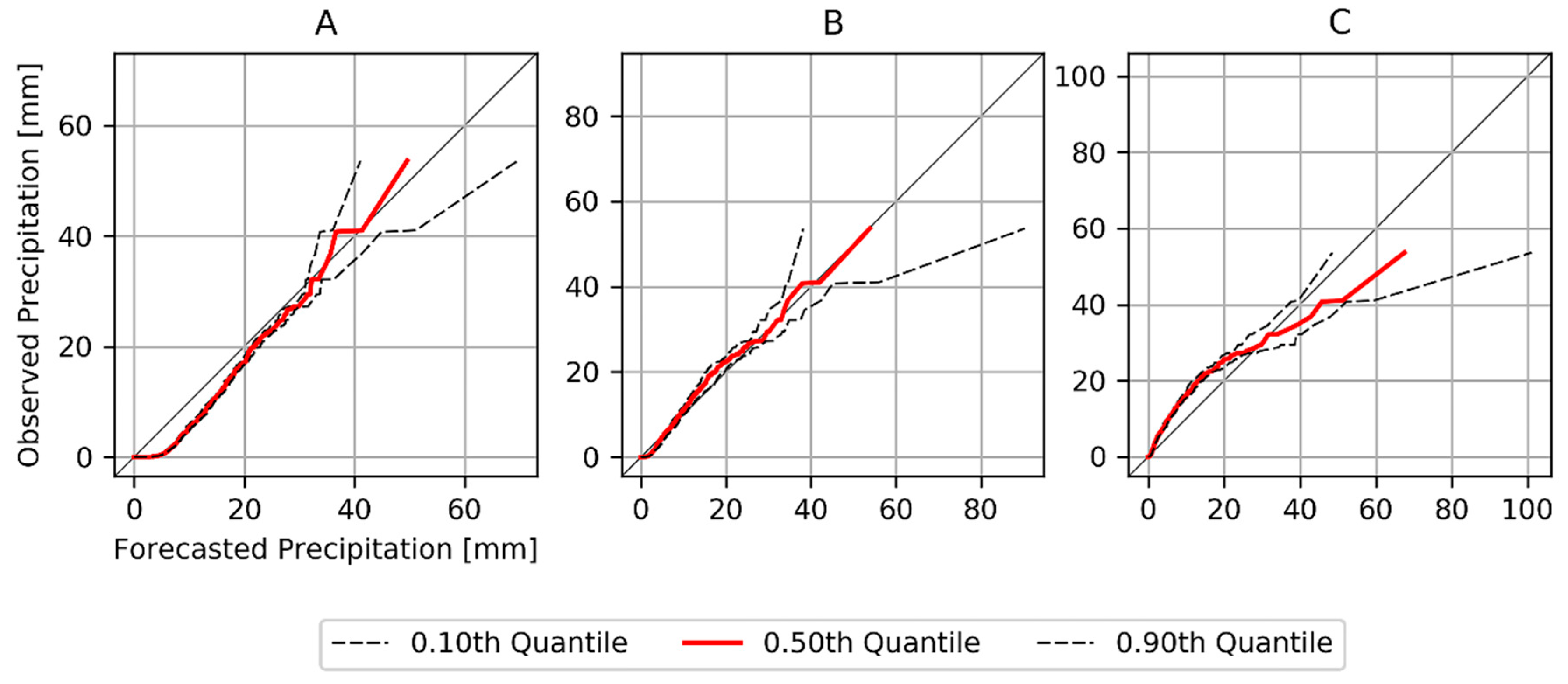
3.1. Bias Correction of Ensemble Precipitation Forecasts

Precipitation information from global models used in weather forecasting and climate prediction are characterized by systematic deviations from observations so that the observed precipitation climatology for a given geographical region is often not well reproduced. This problem is shown for different climatological zones in West Africa for example by [13]. They analyzed the precipitation hindcasts of CFSv2 in comparison to the Global Precipitation Climatology Centre reanalysis dataset over a period of more than 25 years (1983–2009). Moreover, the precipitation bias of climate models can also reduce the reliability of hydrological or agricultural model simulations, if the precipitation simulations are used without any corrections. Therefore, different bias correction techniques were developed in the past to eliminate systematic model deviations and to better match the observed climatology for a given region. A recent overview is presented in [45] and applications for the West African monsoon are given in [13,46]. In this study, the quantile–quantile transformation following [22] and [47] is applied to adapt the distribution of the hindcasts ensemble (SYS4) to the observed climatological distribution (CHIRPS). In this work, the procedure is performed for each ensemble member and grid point separately using the daily time series as follows:
  • Sort the daily observed values x = {   x 1 ,   x 2 ,   ,   x n   } for the investigation period (1 February–31 February, 2000–2010) in an ascending order.
  • Determination of the rank R x i for each observation with i = 1 , 2 , , n and n = number of observations.
  • Determining the empirical cumulative distribution function of the observations F x by calculating the cumulative frequencies p i for each observation using the formula p i =   R x i / ( n + 1 ).
  • Sort the daily forecast values y = {   y 1 ,   y 2 ,   ,   y n   }   of an ensemble member for the investigation period (1.02–31.08, 2000–2010) in an ascending order.
  • Determination of the rank R y i for each forecast with i = 1 , 2 , , m and m = number of forecasts.
  • Determining the empirical cumulative distribution function of the forecasts   F y by calculating the cumulative frequencies q i for each forecast using the formula q i =   R y i / ( m + 1 ) .
  • Determine the corrected prediction value y i for each q i with the inverse cumulative distribution function of the observations y i =   F x 1 ( q i ) .
  • Repeat steps 4–7 for each ensemble member and each grid point.
Figure 3 shows an example of a quantile–quantile transformation of daily precipitation amounts to better understand the approach described above. Here y(t) corresponds to the original value of the forecast and y’(t) to the forecast value corrected by the inverse cumulative distribution function of the observation.
The analysis of the joint distribution of the forecasts (SYS4) and the observations (CHIRPS) is done by a quantile–quantile plot, in which the daily sorted forecasted and observed precipitation values are represented in a coordinate system against each other. At this point it should also be mentioned that due to the grid-based determination of the ORS in Section 3.2, the focus is on the data of the individual grid points and therefore no temporal or spatial aggregation is performed. Accordingly, this analysis evaluates three grid points, each representative for different climate regions of the study zone: Guinea Coast (A), Sudan (B) and Sahel (C). Figure 4 shows the quantile plots for selected grid points of these zones for the 15 SYS4 ensemble members using selected quantiles (Q10, median, Q90). The distribution of the CHIPRS observations is relatively good captured by the SYS4 ensemble members, in particular for the Sudan zone. However, the analysis also reveals several systematic deviations between the SYS4 ensemble and the CHIRPS observations. For instance, smaller precipitation amounts (<20 mm/d) are strongly overestimated by the SYS4 ensemble for the grid point A located in the Guinean coasts. In addition, the SYS4 ensemble shows a quite diverse picture for the Sahel region with underestimations of the lower precipitation range (<30 mm) and overestimations of the upper precipitation range (>30 mm). Overall, Figure 4 indicates that the intra-ensemble biases of raw SYS4 forecasts are comparable to CHIRPS, i.e., the CHIRPS lies within the distribution of the SYS4 ensemble simulations. For high precipitation values, the SYS4 distributions are wider compared to small values. This is to be expected due to the fact that high precipitation values are less frequent and might be affected more heavily by stochasticity, coming from uncertainties from the model initial conditions and other limitations of the model such as parameterization options and non-adequate model equations [48]. Due to the systematic deviations for the small precipitation values (as discussed above), a statistical bias correction is applied in this study. This bias correction is done for each ensemble member separately.

3.2. Calculation of the ORS Dates Using Fuzzy Rules

There are several definitions for the determination of ORS for the West African monsoon system. An overview of these methods is given in [49]. Ref [20] divides the definitions into two categories:
  • ORS is defined by local precipitation events and is based on dry and wet periods.
  • ORS is defined by large-scale changes of the WAM system, indicated by e.g., circulation patterns or specific atmospheric variables like long-wave radiation fluxes.
In this study, the approach by [17] was applied, which belongs to the first category proposed by [20]. The approach of [17] is based on the ORS definitions of [50]. In [50] the ORS is defined as the first day of the year in which the following three conditions occur simultaneously:
  • The accumulated sum of precipitation in five consecutive days is at least 25 mm.
  • Within this pentad, at least two more days must exceed a precipitation amount of 1 mm.
  • There is no period of consecutive 7 dry days or longer within the next 30 days (false start criterion). A dry day is defined as a day with less than 1 mm precipitation.
A shortcoming of the approach by [50] is its binary logic. An accumulated precipitation sum of 24.9 mm is not identified as the onset of the rainy season although only 0.1 mm is missing to fulfill the criteria. Since many other ORS approaches rely on binary logics, [17] introduced fuzzy rules for a more smoothed transition of the applied conditions. This ORS fuzzy-logic were used by several other investigations, as well [2,51]. The membership functions of the fuzzy rules used in this study are shown in Figure 5. For example, for condition 1, accumulated precipitation amounts of less than 18 mm receives a membership value of 0, and above 25 mm a 1. In the range between 18 and 25 mm, normalized values between 0 and 1 are assigned by linear interpolation. Thus, the probabilities of being interpreted as ORS are increasing with precipitation rates larger than 18 mm. A similar membership function is applied to condition 2, which is supposed to exclude single rainfall events to be misinterpreted as ORS. It must be noted that the membership functions were optimized for the Volta Basin of West Africa [17], and therefore could be assumed to be reasonable for our study area.
Due to the runtime length (seven months) of SYS4 and the late ORS within the Sahel zone, the false start criterion (condition 3) is not included in this study. However, we found that the false start criterion had only little impact on the ORS patterns. The criterion was evaluated with CHIRPS over the study period and each grid cell. The ORS only shifted in 14.1% of the cases (not shown). False starts occurred all over the study region and it was not only a problem of the northern parts. To avoid this, a smaller domain must be used, the runtime length of SYS4 needs to be extended or the fuzzy rules need to be optimized for operational applications. Therefore, a complete application of the approach should be carried out based on these evaluation results in further studies.
The ORS is met if the multiplied values of both membership functions (γ1 and γ2) exceeds a given threshold value γ t   . Any variation of the γ t   can influence the ORS calculation and can therefore avoid that no ORS date is defined for a particular year. This is a common problem for other ORS definition. In this study a threshold value of γ t   = 0.5 is used for the calculation of the ORS dates.

3.3. Verification of the Spatial ORS Fields

The ORS is calculated according to the aforementioned definitions for each grid point over all ensembles and CHIRPS observations, as well. The verification of the ORS forecasts is on the one hand performed spatially for each year over the entire study domain (spatial verification), and on the other hand temporally for each grid cell [23] over the entire study period (temporal verification). Considering the grid-based development of the ORS index in Section 3.4, it is important that the data is evaluated both temporally for each grid cell and spatially for each year.
The spatial verification of the ORS fields is performed by calculating the Pearson’s correlation coefficient (r), the mean absolute error (MAE) and the anomaly correlation coefficient (ACC) between the forecasted and the corresponding observed ORS. MAE and r are calculated for each ensemble member j and time step t using Equations (1) and (2).
M A E j   ( t ) =   1 M i = 1 M | y i j ( t ) o i ( t ) | ,
r j ( t ) =   i = 1 M ( y i j ( t ) y ¯ j ( t ) ) ( o i ( t ) o ¯ ( t ) ) i = 1 M ( y i j ( t ) y ¯ ( t ) ) 2   i = 1 M ( o i ( t ) o ¯ ( t ) ) 2 ,
where M corresponds to the number of grid points, y i j to the ORS forecast value at grid cell i of ensemble member j and o i to the corresponding observed ORS value. The mean observed and forecast ORS values of ensemble member j of the data sets are given by y ¯ and o ¯ . The Pearson’s correlation coefficient and related measures like coefficient of determination are one of the most popular scores used for model validation. The correlation coefficient is also frequently used for the verification of spatial fields as outlined by [19] and for comparison of atmospheric fields as a measure for pattern similarity [52]. The Pearson correlation coefficient is also a measure for the skill of a forecast system as shown by [53]. However, unlike other popular skill scores for continuous variables (e.g., the mean squared error skill score), it measures the potential skill of the forecast system as defined by [53] without any unconditional bias.
The ACC is another common measure used specifically for spatial forecast verification [19,23]. First, the anomalies values of the forecasts y i j and observations o i are calculated with y i j =   y i j o ¯ r and o i =   o i o ¯ r where y i is the ORS forecast value at grid cell i and o i to the corresponding observed ORS value. The mean observed ORS values of the climatological reference period (1981–2010) are given by o ¯ r . Then, the Pearson correlation is applied using the anomaly values. The score measures therefore how good the correspondence is between the predicted and the observed anomaly fields, which is highly important for climate model evaluation.
In addition to the spatial verification, the MAE and r are calculated for each time series of a grid cell and over the respective study period to perform a temporal verification of the ORS forecast. Afterwards, an averaging of the (skill) scores from the individual 15 ensemble members takes place. It should therefore be mentioned that the mean score is not indicative of the performance of the ensemble mean.

3.4. Calculation of the ORS Index

In order to better interpret ensemble-based ORS forecasts, an index for the ORS dates is proposed in this study. The approach is based on probabilistic forecasts for the ORS date computed for climatologically equiprobable categories. The calculation of the ORS index for these categories is based on the following formula:
O R S I = k = 1 K g k p k ,
where p k is the forecast probability of k-th category, g k is the corresponding weight of k-th category, K is the number of climatologically equiprobable categories. The weight g k is computed by calculating the difference between the bin centre of k-th category and the median of uniformly distributed forecast probabilities, which is 0.5. The value of g k can range between 1 and −1. A forecast probability of extreme categories therefore receives a higher weight in comparison to categories close to the middle category. In the case of an odd number of equiprobable categories like tercile-based categories, the forecast probability of the middle category receives no weight.
In this study the ORS index is computed for tercile-based probabilistic forecasts of the ORS dates. Tercile-based probabilistic forecasts are the most common format in seasonal forecasting [23]. The values of the tercile-based ORS index ranges between 33. 3 ¯ and 33. 3 ¯ , where negative (positive) ORS values indicate a late (early) onset and corresponding distribution of the forecast probabilities is left skewed (right skewed). The minimum (maximum) ORS value of 33. 3 ¯ ( 33. 3 ¯ ) is reached, if all ORS members belong to the category below average (above average) with p 3 = 100 % ( p 1 = 100 % ) and p 2 = p 1 = 0 % ( p 3 = p 2 = 0 % ). The weights for the computation of the ORSI values for tercile-based forecast are g 1 = 1 3 ,   g 2   = 0 and g 3   =   1 3 . The forecast probability for the near-normal category receives therefore no weight. The calculation of the ORSI only relies on the forecast probability for above normal and below normal. Climatological forecasts with equally distributed forecast probabilities ( p 1   = 33. 3 ¯ % ,     p 2   = 33. 3 ¯ % and p 3   = 33. 3 ¯ % ) are indicated by an ORSI value of zero. The same applies also for symmetric distributed forecast probabilities (e.g., p 1   = 20 % ,   p 2   = 60 % and p3 = 20%) and if all members belong to the category near average (p1 = 0%, p2 = 100% and p 3   = 0 % ). Thus, the ORS index provides information about an early, mean and late onset of the rainy season. However, it cannot distinguish between climatological forecasts and forecasts where a normal onset is more likely.
In the following, the methodology for probabilistic forecasting of the ORS dates is listed as an example for a grid cell:
  • Calculation of the observed ORS dates from CHIRPS for the period from 1981–2010.
  • Determination of the quantiles Q 1 3 and Q 2 3 from the observed ORS dates to define the tercile-based ORS categories.
  • Calculation of the ORS dates from the bias-corrected SYS4 precipitation hindcasts for each ensemble member of a given year.
  • Classification of the 15 ORS ensemble members into the three tercile-based categories: Below average, if yij (t) < Q 1 3 , near average, if Q 1 3   ≤ yij (t) ≤ Q 2 3 and above average, if yij (t) > Q 2 3 .
  • Calculation of the corresponding forecast probabilities pk for each ORS category.
  • Calculation of the ORS index value based on Equation (3).
  • Step 3 to 6 are repeated, if the forecasts probabilities are determined for other years.

4. Results and Discussion

4.1. Spatiotemperal Verification of the ORS Fields

The spatial accuracy of the ORS forecasts is shown in Figure 6 in terms of the MAE. The MAE was computed for each ensemble member and based on this information a box-plot diagram was produced for each year. Thus, the mean of the box plots shows the average accuracy of the ensemble forecasts for a given year and the box-plot spread the performance differences between the ensemble members. The mean MAE over the study period is 23.3 days, which indicates a relatively low accuracy for the prediction of the ORS dates in this region. This outcome can be expected because the prediction of precipitation characteristics on a much coarser temporal scale (e.g., monthly or seasonal precipitation amounts) is already characterized by low performance as shown by [13]. Moreover, seasonal forecasting of specific daily precipitation characteristics like ORS dates is a much more challenging task in comparison to seasonal forecasting of monthly or seasonal precipitation amount (or other meteorological variables like temperature). Reasons are the inherent high uncertainty of long-range forecasts products like seasonal forecasts and the high stochastic character of daily precipitation events, in particular in monsoonal regions like West Africa. Another reason is the uncertainty coming from the reference products used for comparison. This is shown e.g., by [51] for the calculation of the ORS dates for West Africa. Figure 6 also shows strong variations of the forecast performance of the ORS dates for the different years indicated by the mean and the spread of the box-plot diagrams. For some years the ORS forecasts were much better (e.g., 2007) in comparison to other years (2005).
The inter-annual variation of the performance can be also a pure random artifact due the low sample size of 15 ensemble members. To prove this hypothesis, statistical tests using a Student’s t-test for paired samples and a modification of Student’s t-test for unequal variances, the Welch’s t-test [54,55], are applied to evaluate whether the mean values of two MAE samples (e.g., 2007 and 2005) are significantly different from each other. More information how the statistical tests are exactly used in this study is given in the Appendix A. The statistical tests partially confirm the aforementioned hypothesis. However, the outcomes of the t-tests also indicate that the mean MAE values are significantly different from each other for pairs with very different means (like 2007 and 2005) indicating that the inter-annual variation of the performance is not a pure random artifact.
The association between the predicted and observed ORS fields is shown in Figure 7 for the Pearson’s correlation coefficient. The outcomes of this study show that the average of the correlation coefficients is 0.79 with a maximum value of 0.92 for the year 2006. Only the year 2005 falls strongly out of the upper correlation range because several statistics of the box plot diagram like the first quartile (0.75) and the minimum value (0.40) show the smallest but still a moderate to high correlation. Since the Pearson correlation coefficient is not only a measure of association between two fields but also a measure of the skill, the ORS prediction seems to be very skillful for this region. However, most of the skill is artificial due to strong seasonality of the ORS dates as a result of the northward migration of the WAM system during the boreal spring and early summer. The calculation of the anomalies for the forecasts and observed ORS values removes the seasonality of the ORS fields. The resulting anomaly patterns have a much smaller association, but they still have a slight positive correlation for most of the members (Figure 8). Moreover, the calculation of the significance threshold for the ACC scores based on a Student’s t-test (α = 0.10, n = 185) indicates only for two years, namely 2000 and 2001, a significant skill for the majority of the ensemble members. This example demonstrates the importance of selecting an appropriate skill score for the verification of the spatial ORS fields. Otherwise the forecasts performance for the ORS dates could be highly misinterpreted for this region. Figure 8 also shows that the quality of the ORS forecast strongly varies for the different years like for the other scores. There are several years when the majority of the ORS ensemble members have a negative ACC. This is case for 2009 where 13 out of 15 ensemble members are negative and the ACC mean is −0.11 and ACC has a minimum value of −0.44. On the other hand, there are also several years when most of the ensemble members have a positive ACC. For example, 14 out of 15 members are positive ACC value for 2001. For this year the ACC mean is 0.13 and the maximum ACC of the ensemble reaches a value of 0.48.
In addition, a temporal verification of the ORS forecasts is performed in this study. The verification measures are calculated for each grid cell by comparing the predicted ORS time series with a time series of the ORS observations. The verification measures are calculated for each ensemble member separately and afterwards an averaging of this sample is conducted. The outcome of this calculation is shown for the MAE (a), r (b) and bias (c) in Figure 9. It shows strong regional differences regarding the accuracy of the ORS forecast. The MAE values gradually decrease from the South to the North with a MAE of approximately 15 days in the southwestern part of the study domain near the Guinean coastline and more than 35 days in the northern part of the study domain. Thus, the accuracy of the ORS forecasts is much higher for the Guinean zone in comparison to the Sudan-Sahel region. Several studies already showed that seasonal precipitation forecasts for West Africa have usually a higher performance for the Guinean zone compared to the poleward located climate zones like the Sudan-Sahel or Sahel (e.g., [11,22]). Ref [22] mentions that those regions have a higher skill where precipitation is stronger interlinked with oceanic surface conditions. Another explanation for the lower model accuracy in the Sahel region can be the higher stochastic nature of the precipitation events in this region compared to the Guinean zone since most of the rainfall is the result of convective systems in the Sahel region (see [56]; and references herein). However, the gradual decline of the MAE values can also be a purely operational effect. The ORS dates in the Guinean zone are based on much shorter lead times in comparison to the ORS dates in the Sahel zone, and the accuracy of the ORS prediction should theoretically decrease with shorter lead times.
The correlation map shows a positive skill for most part of the Guinea zone. This region is also characterized by the highest skill (up to 0.40 and more) since the MAE and the bias values are relatively low compared to the other regions. The northern parts of the study domain show also a slight positive skill between the predicted and observed time series, although the accuracy of the ORS forecast is relatively low. The low accuracy is mainly the result of the strong unconditional biases in this region as shown in Figure 9c. The MAE value is negatively influenced by a bias, which is not the case for the correlation measure [53]. Thus, the correlation indicates the model skill in term of bias-free products and it is a verification measure for the potential skill of ORS forecasts. However, it must be noted that due to the small sample size (11 years), the significance threshold for the Pearson correlation is r = 0.39 (based on a Student’s t-test, α = 0.10, n = 11). Thus, for most of parts of the study domain the model skill is not statistically significant. Only for several grid cells next to the Guinean coast this threshold is reached or exceeded.

4.2. Visualisation of the ORS Fields

The ensemble-based forecasts of the ORS dates are shown in Figure 10 for the year 2001. We selected this year because according to the MAE and ACC values computed in the previous section, 2001 is the best year in terms of forecast accuracy and skill. Moreover, the year 2001 is also characterized by a rather special observational ORS pattern with a late ORS in the Guinean zone and an early ORS in the Sahel zone. This pattern is shown in Figure 11c computed as the differences between the absolute ORS values minus the climatological mean. Thus, positive values in Figure 11 indicate a late onset (red pixels, near the Guinean coast, mostly below 10° N) and negative values an early onset (blue pixels, mostly above 10° N).
The ORS forecasts in Figure 10 are based on the ensemble mean (middle panel), both terciles (right and left panel) and the inter-quantile range to illustrate the forecast uncertainty. Quantile-based forecasts are a straightforward way for visualization of ensemble-based forecasts and are often used to illustrate forecast uncertainties for precipitation, but also for other hydro-meteorological variables. The quantile-based approach is already used by [13] to visualize ORS predictions. This graphical approach should be also preferred in comparison to plotting the spatial fields of all ensemble members. This latter approach is often named as spaghetti plots in ensemble forecasting (e.g., [57,58,59] and it has the disadvantage that the plots became very confusing, in particular for large ensemble sizes and higher lead times.
The quantile-based ORS maps show a clear north–south gradient of the ORS dates. In this respect, a relatively realistic pattern is produced for the forecasts. The information based on the terciles can also be interpreted as an early and late ORS date. The difference between the late and the early ORS dates is an estimation of the forecast uncertainty. The uncertainty is quite large although only 1/3 of the ensemble is used for the illustration. Figure 10d also indicate that the uncertainty increases from the Guinean coastline to the Sahel zone due to the different lead times and other reasons as discussed in the previous section. Moreover, a comparison of Figure 10a–c with Figure 11a reveals that many observations are not enclosed by the selected uncertainty interval. The approach produces for the southern parts of the domain too early ORS dates and too late ORS dates for the northern part of the domain. This shows that the selected quantiles are too narrow to enclose all observations. If more extreme quantiles (e.g., Q90 and Q10) are used for the calculation of the late and early ORS dates, the observations will be better enclosed by the uncertainty interval. However, this will also strongly increase the range of the illustrated forecast uncertainty.
Another format for the visualization of ensemble-based ORS forecasts are probabilistic forecasts based on climatologically equiprobable categories shown in Figure 12. In this study, the forecast probabilities are calculated for each grid cell for tercile-based categories over the entire domain. Climatological average conditions (Figure 11b) are indicated by uniformly distributed forecast probabilities (1/3 for all three categories). For the central and northern parts of the study region, the ORS is forecasted to be earlier, because the forecast probabilities are much higher for “below-normal” than the average conditions (1/3) and much lower for the other categories. For the southern parts of the study region, it is vice versa, with much higher probabilities for “above normal” and ORS is expected to be late. However, a correct interpretation of the tercile-based categories is for many users not straightforward since forecast probabilities of climatologically equiprobable categories needs to be considered jointly and a good statistical background is therefore needed. For further discussion regarding this issue we refer to the study of [11] and the references herein.
An alternative way for illustrating the forecast probabilities of climatologically equiprobable categories is the ORS index proposed in Section 3.4. This index is displayed for the year 2001 in Figure 13 based on the forecast probabilities given in Figure 12. At a glance, the ORS index provides information on an early (green, ORSI > 0), normal (yellow ORSI ~ 0) and late (red, ORSI < 0) ORS. The ORSI therefore summarizes the information from the three probabilistic patterns and is thus much easier to interpret than Figure 12. It therefore provides a simple alternative to illustrate whether an early or late ORS is forecasted for the coming rainy season. For our specific example, the index shows strong negative values up to –30 for the Guinean coast indicating a late ORS for that region, while for the Sahel zone the opposite signal is predicted (a late onset with ORSI values up to 30). Thus, the predicted ORSI patterns show very similar large-scale features as the observed ORS anomalies shown in Figure 11c.

5. Summary and Conclusions

This work presented a statistical approach for seasonal forecasting of the onset of the rainy season using precipitation forecasts of a GSEPS. The basis of this approach was a quantile–quantile transformation for removing biases from the precipitation ensemble, a fuzzy-rule based approach for calculation of the ORS date and several graphical methods for an improved visualization of ensemble-based ORS forecasts. As outlined in the methodology part of the work, the different components of the approach were modular and could therefore be replaced by other methods (i.e., downscaling or ORS approaches) and datasets (i.e., GSEPS forecasts and observations). Moreover, the approach could be relatively easily transferred to other geographical regions of the world and extended to crucial rainfall characteristics like the cessation and the length of the rainy season. The presented approach has also the advantage that it is not very CPU demanding and requires only a single variable for the downscaling process. Unlike many other downscaling approaches, it might be better operationally applicable to forecasting centers in development countries where bandwidth and computing power are often limited.
In this study we also performed a first evaluation of the ORS forecasts by employing various verification measures and methods to determine the performance of the approach in space and in time. This analysis illustrated that forecasting ORS dates several months in advance was a major challenge. The ORS forecasts were associated with large uncertainties due to the inherent high uncertainty of seasonal forecasts and other reasons like the high stochastic nature of daily precipitation in West Africa. We also illustrated in this study the importance of selecting appropriate performance measures for verification of the spatial ORS fields to remove seasonal dependencies. This was done by using the anomaly correlation coefficient. Since the focus was on spatial verification of the ORS fields, other methods for verification of probabilistic forecast like the continuous ranked probability score [60] were not yet employed. However, this type of forecast verification is needed to get a better insight regarding the quality of probabilistic seasonal ORS forecasts. In addition, verification techniques for determining the economic value should be applied in future studies to determine another type of forecast goodness, i.e., the forecast value (e.g., [19]). This is needed to demonstrate how valuable the ORS forecast is for a particular end user. Recent examples towards this kind of verification are presented e.g., in [11,61]. The selected spatial verification methods applied in this study were also relatively strict and imply a perfect forecast of the ORS fields in space and time, in particular the MAE. This basic assumption should be further examined in future studies by the selection of alternative spatial verification methods. These new methods can be found, for example, in [23,62].
We also tested different forecasts formats for visualization of probabilistic ORS forecasts. These approaches range from quantile-based ORS forecasts, over climatologically equiprobable categories to a new ORS index for indicating an early or late ORS. Since the ORS index is a joint measure of categorical forecasts, it is much easier to understand than the common formats used in seasonal forecasting. Moreover, the ORS index was applied in this study to tercile-based categories but can be also used for forecasts for more than three categories and to other seasonal forecasts variables. The index provides therefore an important alternative to the current forecast formats used in seasonal forecasting.
There were several limitations of the presented methodology. Possible improvements in future studies are:
  • Better adapting the ORS approach to the location-specific conditions in the region, i.e., considering the heterogeneous rainfall conditions across the region. This can be achieved by coupling the ORS approach to a process-based crop model to derive location-specific planting rules (ORS criteria), as done in [2,63]. Based on seasonal predictions, it is also possible to incorporate the false-start criterion in the ORS predictions;
  • Testing the skills of other GSEPS such as the Climate Forecast System Version 2 or the ECMWF SYS5, which is e.g., improved in terms of the spatial resolution and the number of ensemble members compared to the SYS4 [64]. Since the probabilistic forecast depends strongly on the size of the ensemble members (e.g., [64]), the increase of the ensemble members may possibly lead to improved ORS predictions;
  • Incorporating longer lead times in the analysis. Longer lead times would increase preparation time for farmers. On the other hand, increasing the lead time would result in reduced forecast periods for the rainy season;
  • Further reducing the biases in the forecasts, either by improving the statistical bias correction method or by dynamically downscaling the forecasts. The former could e.g., be achieved by applying the corrections separately for the different months (e.g., [65]) or for different large-scale atmospheric circulation patterns (e.g., [66]).
In general, more precise ORS forecasts will possibly impact on the farmer’s tactical decision such as the timing for planting, the types crops and the varieties to grow, i.e., long or short duration varieties.

Author Contributions

The method of this work was designed by J.B., P.L. and M.R. The state-of-the-art of seasonal forecasting in West Africa was reviewed by M.W., S.S., J.B. and M.R. The formal analysis (data preparation, programming, validation and visualization) was done by M.R. H.K. was responsible for supervision and funding acquisition. Writing and original draft preparation was jointly done by M.R. and J.B. Final reviewing, writing and editing was done by all authors.

Funding

This work was part of the WASCAL (West African Science Service Centre on Climate Change and Adapted Land Use, 01LG1202C1) and SaWaM (Seasonal Water Resources Management in Semiarid Regions: Application-oriented Transfer of Regionalized Global Information) project funded by the Federal Ministry of Education and Research in Germany.

Acknowledgments

We want to acknowledge Christoph Lorenz for preparing and providing the SYS4 hindcasts data for our study region of interest. We acknowledge support by Deutsche Forschungsgemeinschaft and Open Access Publishing Fund of Karlsruhe Institute of Technology.

Conflicts of Interest

The authors declare no conflict of interest. The funders had no role in the design of the study; in the collection, analyses, or interpretation of data; in the writing of the manuscript, or in the decision to publish the results.

Appendix A

A basic assumption for the application of the Student’s t-test or Welch’s t-test is that the MAE samples are normally distributed for each year. To check this assumption, a Shapiro–Wilk test [67] on the MAE samples was performed, which are shown in Table A1. In addition, the Levene’s test [68] for equality of variances (e.g., H 0   : σ 2007 2 =   σ 2005 2 ) was used to decide whether to use Student’s t-test or Welch’s t-test. All samples are normally distributed (Table A1), but some pairs of the year’s show inequality of variances (Table A2). Since Student’s t-test cannot be used for inequality of variances (e.g., σ 2000 2   σ 2002 2 ) the Welch’s t-test was applied. For all combinations of years with equal variances Student’s t-test (e.g., σ 2000 2 =   σ 2001 2 ) was used (Table A3).
Table A1. Shapiro–Wilk test for normality, bold print if H0 was accepted at α = 0.05.
Year20002001200220032004200520062007200820092010
Shapiro-Wilk test0.9620.9530.9130.9410.9480.9680.8880.9450.9090.9760.912
Table A2. Levene’s test for equality of variances, bold print if H0 was accepted at α = 0.05.
Year20002001200220032004200520062007200820092010
20000.00000.68574.44013.23950.445711.412410.46890.00464.21944.77320.2915
20010.68570.00002.44021.34790.01287.50996.78620.97651.69502.05750.1180
20024.44012.44020.00000.24682.58070.60760.46804.96390.30730.20463.3129
20033.23951.34790.24680.00001.48161.96001.66803.78980.00060.00822.1308
20040.44570.01282.58071.48160.00007.61056.89920.63381.83932.20290.0415
200511.41247.50990.60761.96007.61050.00000.009912.86512.38252.03909.4714
200610.46896.78620.46801.66806.89920.00990.000011.79912.02971.71658.6121
20070.00460.97654.96393.78980.633812.865111.79910.00005.14845.78920.4753
20084.21941.69500.30730.00061.83932.38252.02975.14840.00000.01632.7800
20094.77322.05750.20460.00822.20292.03901.71655.78920.01630.00003.2528
20100.29150.11803.31292.13080.04159.47148.61210.47532.78003.25280.0000
Table A3. Two sample t-test for equal means (equal variances)/Welch’s t-test (unequal variances), bold print if H0 was accepted at α = 0.05.
Year20002001200220032004200520062007200820092010
20000.00001.8406−0.21890.18160.1690−2.3839−0.78482.11290.4895−0.88310.9980
2001−1.84060.0000−1.3634−1.1451−1.5163−3.3723−1.8394−0.0538−0.9283−2.1992−0.8811
20020.21891.36340.00000.31710.3161−1.7477−0.46271.41190.5372−0.44300.8145
2003−0.18161.1451−0.31710.0000−0.0500−2.1811−0.80061.19850.2338−0.85090.5113
2004−0.16901.5163−0.31610.05000.0000−2.3958−0.85541.67830.3311−0.95610.7306
20052.38393.37231.74772.18112.39580.00001.23993.51432.43881.50092.9086
20060.78481.83940.46270.80060.8554−1.23990.00001.90461.02260.08791.3350
2007−2.11290.0538−1.4119−1.1985−1.6783−3.5143−1.90460.0000−0.9712−2.3518−0.9699
2008−0.48950.9283−0.5372−0.2338−0.3311−2.4388−1.02260.97120.0000−1.12590.2509
20090.88312.19920.44300.85090.9561−1.5009−0.08792.35181.12590.00001.5821
2010−0.99800.8811−0.8145−0.5113−0.7306−2.9086−1.33500.9699−0.2509−1.58210.0000

References

  1. Dobor, L.; Barcza, Z.; Hlásny, T.; Árendás, T.; Spitkó, T.; Fodor, N. Crop planting date matters: Estimation methods and effect on future yields. Agric. For. Meteorol. 2016, 223, 103–115. [Google Scholar] [CrossRef]
  2. Waongo, M.; Laux, P.; Traoré, S.B.; Sanon, M.; Kunstmann, H. A crop model and fuzzy rule based approach for optimizing maize planting dates in Burkina Faso, West Africa. J. Appl. Meteor. Climatol. 2014, 53, 598–613. [Google Scholar] [CrossRef]
  3. Nicholson, S.E. Climatic and environmental change in Africa during the last two centuries. Clim. Res. 2001, 17, 123–144. [Google Scholar] [CrossRef] [Green Version]
  4. Nicholson, S.E.; Funk, C.; Fink, A.H. Rainfall over the African continent from the 19th through the 21st century. Glob. Planet. Chang. 2018, 165, 114–127. [Google Scholar] [CrossRef]
  5. Adegoke, J.; Bamba Sylla, M.; Bossa, A.; Ogunjobi, K.; Adounpke, J. On the 2017 rainy season intensity and subsequent flood events over West Africa. In Regional Climate Change Series: Floods; WASCAL Publishing: Accra, Ghana, 2019; pp. 10–14. [Google Scholar]
  6. Markantonis, V.; Farinosi, F.; Dondeynaz, C.; Ameztoy, I.; Pastori, M.; Marletta, L.; Ali, A.; Carmona Moreno, C. Assessing floods and droughts in the Mékrou River basin (West Africa): A combined household survey and climatic trends analysis approach. Nat. Hazards Earth Syst. Sci. 2018, 18, 1279–1296. [Google Scholar] [CrossRef]
  7. Munich Re. NatCat Service; Munich Re: Munich, Germany, 2019. [Google Scholar]
  8. Ingram, K.T.; Roncoli, M.C.; Kirshen, P.H. Opportunities and constraints for farmers of West Africa to use seasonal precipitation forecasts with Burkina Faso as a case study. Agric. Syst. 2002, 74, 331–349. [Google Scholar] [CrossRef]
  9. Amegnaglo, C.J.; Anaman, K.A.; Mensah-Bonsu, A.; Onumah, E.E.; Gero, F.A. Contingent valuation study of the benefits of seasonal climate forecasts for maize farmers in the Republic of Benin, West Africa. Clim. Serv. 2017, 6, 1–11. [Google Scholar] [CrossRef]
  10. Ouédraogo, M.; Barry, S.; Zougmoré, R.; Partey, S.; Somé, L.; Baki, G. Farmers’ willingness to pay for climate information services: Evidence from Cowpea and Sesame producers in Northern Burkina Faso. Sustainability 2018, 10, 611. [Google Scholar] [CrossRef]
  11. Bliefernicht, J.; Waongo, M.; Salack, S.; Seidel, J.; Laux, P.; Kunstmann, H. Quality and value of seasonal precipitation forecasts issued by the West African regional climate outlook forum. J. Appl. Meteorol. Climatol. 2019, 58, 621–642. [Google Scholar] [CrossRef]
  12. World Meteorological Organization (WMO). Regional Climate Outlook Forums. Available online: https://library.wmo.int/doc_num.php?explnum_id=3191 (accessed on 27 June 2019).
  13. Siegmund, J.; Bliefernicht, J.; Laux, P.; Kunstmann, H. Toward a seasonal precipitation prediction system for West Africa: Performance of CFSv2 and high-resolution dynamical downscaling. J. Geophys. Res. Atmos. 2015, 120, 7316–7339. [Google Scholar] [CrossRef]
  14. African Centre of Meteorological Application for Development (ACMAD). Regional climate outlook forum PRESASS-06. Available online: http://acmad.net/rcc/atelier/bulletin_PRESASS06_eng.pdf (accessed on 27 June 2019).
  15. Omotosho, J.B.; Balogun, A.A.; Ogunjobi, K. Predicting monthly and seasonal rainfall, onset and cessation of the rainy season in West Africa using only surface data. Int. J. Climatol. J. R. Meteorol. Soc. 2000, 20, 865–880. [Google Scholar] [CrossRef]
  16. Laux, P.; Wagner, S.; Wagner, A.; Jacobeit, J.; Bárdossy, A.; Kunstmann, H. Modelling daily precipitation features in the Volta Basin of West Africa. Int. J. Climatol. J. R. Meteorol. Soc. 2009, 29, 937–954. [Google Scholar] [CrossRef] [Green Version]
  17. Laux, P.; Kunstmann, H.; Bárdossy, A. Predicting the regional onset of the rainy season in West Africa. Int. J. Climatol. J. R. Meteorol. Soc. 2008, 28, 329–342. [Google Scholar] [CrossRef]
  18. Omotosho, J.B. Long-range prediction of the onset and end of the rainy season in the West African Sahel. Int. J. Climatol. 1992, 12, 369–382. [Google Scholar] [CrossRef]
  19. Wilks, D.S. Statistical Methods in the Atmospheric Sciences; Academic Press: Cambridge, UK, 2011; ISBN 0123850223. [Google Scholar]
  20. Vellinga, M.; Arribas, A.; Graham, R. Seasonal forecasts for regional onset of the West African monsoon. Clim. Dyn. 2013, 40, 3047–3070. [Google Scholar] [CrossRef]
  21. Saha, S.; Moorthi, S.; Wu, X.; Wang, J.; Nadiga, S.; Tripp, P.; Behringer, D.; Hou, Y.-T.; Chuang, H.-Y.; Iredell, M. The NCEP climate forecast system version 2. J. Clim. 2014, 27, 2185–2208. [Google Scholar] [CrossRef]
  22. Batté, L.; Déqué, M. Seasonal predictions of precipitation over Africa using coupled ocean-atmosphere general circulation models: Skill of the ENSEMBLES project multimodel ensemble forecasts. Tellus A Dyn. Meteorol. Oceanogr. 2011, 63, 283–299. [Google Scholar] [CrossRef]
  23. Jolliffe, I.T.; Stephenson, D.B. Forecast verification: A Practitioner’s Guide in Atmospheric Science; John Wiley & Sons: Hoboken, NJ, USA, 2012; ISBN 1119961076. [Google Scholar]
  24. Lebel, T.; Diedhiou, A.; Laurent, H. Seasonal cycle and interannual variability of the Sahelian rainfall at hydrological scales. J. Geophys. Res. Atmos. 2003, 108, 1–11. [Google Scholar] [CrossRef]
  25. Fink, A.H. Das Westafrikanische Monsunsystem. Promet 2006, 32, 114–122. [Google Scholar]
  26. Masih, I.; Maskey, S.; Mussá, F.E.F.; Trambauer, P. A review of droughts on the African continent: A geospatial and long-term perspective. Hydrol. Earth Syst. Sci. 2014, 18, 3635–3649. [Google Scholar] [CrossRef]
  27. Salack, S.; Klein, C.; Giannini, A.; Sarr, B.; Worou, O.N.; Belko, N.; Bliefernicht, J.; Kunstman, H. Global warming induced hybrid rainy seasons in the Sahel. Environ. Res. Lett. 2016, 11, 104008. [Google Scholar] [CrossRef]
  28. Taylor, C.M.; Belušić, D.; Guichard, F.; Parker, D.J.; Vischel, T.; Bock, O.; Harris, P.P.; Janicot, S.; Klein, C.; Panthou, G. Frequency of extreme Sahelian storms tripled since 1982 in satellite observations. Nature 2017, 544, 475–478. [Google Scholar] [CrossRef] [PubMed] [Green Version]
  29. Dunning, C.M.; Black, E.; Allan, R.P. Later wet seasons with more intense rainfall over Africa under future climate change. J. Clim. 2018, 31, 9719–9738. [Google Scholar] [CrossRef]
  30. European Centre for Medium-Range Weather Forecasts (ECMWF). System 4 User Guide. Available online: https://www.ecmwf.int/sites/default/files/medialibrary/2017-10/System4_guide.pdf (accessed on 27 June 2019).
  31. Mwangi, E.; Wetterhall, F.; Dutra, E.; Di Giuseppe, F.; Pappenberger, F. Forecasting droughts in East Africa. Hydrol. Earth Syst. Sci. 2014, 18, 611–620. [Google Scholar] [CrossRef] [Green Version]
  32. Winsemius, H.C.; Dutra, E.; Engelbrecht, F.A.; van Archer Garderen, E.; Wetterhall, F.; Pappenberger, F.; Werner, M.G.F. The potential value of seasonal forecasts in a changing climate in Southern Africa. Hydrol. Earth Syst. Sci. 2014, 18, 1525–1538. [Google Scholar] [CrossRef]
  33. Weisheimer, A.; Palmer, T.N. On the reliability of seasonal climate forecasts. J. R. Soc. Interface 2014, 11, 20131162. [Google Scholar] [CrossRef] [PubMed]
  34. Kim, H.-M.; Webster, P.J.; Curry, J.A.; Toma, V.E. Asian summer monsoon prediction in ECMWF System 4 and NCEP CFSv2 retrospective seasonal forecasts. Clim. Dyn. 2012, 39, 2975–2991. [Google Scholar] [CrossRef] [Green Version]
  35. Dutra, E.; Di Giuseppe, F.; Wetterhall, F.; Pappenberger, F. Seasonal forecasts of droughts in African basins using the Standardized Precipitation Index. Hydrol. Earth Syst. Sci. 2013, 17, 2359–2373. [Google Scholar] [CrossRef] [Green Version]
  36. Rodrigues, L.R.L.; García-Serrano, J.; Doblas-Reyes, F. Seasonal forecast quality of the West African monsoon rainfall regimes by multiple forecast systems. J. Geophys. Res. Atmos. 2014, 119, 7908–7930. [Google Scholar] [CrossRef] [Green Version]
  37. Molteni, F.; Stockdale, T.; Balmaseda, M.; Balsamo, G.; Buizza, R.; Ferranti, L.; Magnusson, L.; Mogensen, K.; Palmer, T.; Vitart, F. The New ECMWF Seasonal Forecast System (System 4); European Centre for Medium-Range Weather Forecasts: Reading, UK, 2011. [Google Scholar]
  38. Climate Hazards Group. What Is CHIRPS? Available online: http://chg.geog.ucsb.edu/data/chirps/index.html (accessed on 2 July 2018).
  39. Funk, C.; Peterson, P.; Landsfeld, M.; Pedreros, D.; Verdin, J.; Shukla, S.; Husak, G.; Rowland, J.; Harrison, L.; Hoell, A. The climate hazards infrared precipitation with stations—A new environmental record for monitoring extremes. Sci. Data 2015, 2, 150066. [Google Scholar] [CrossRef]
  40. Dembélé, M.; Zwart, S.J. Evaluation and comparison of satellite-based rainfall products in Burkina Faso, West Africa. Int. J. Remote Sens. 2016, 37, 3995–4014. [Google Scholar] [CrossRef] [Green Version]
  41. Novella, N.S.; Thiaw, W.M. African rainfall climatology version 2 for famine early warning systems. J. Appl. Meteorol. Climatol. 2013, 52, 588–606. [Google Scholar] [CrossRef]
  42. Hsu, K.-L.; Gao, X.; Sorooshian, S.; Gupta, H.V. Precipitation estimation from remotely sensed information using artificial neural networks. J. Appl. Meteorol. 1997, 36, 1176–1190. [Google Scholar] [CrossRef]
  43. Herman, A.; Kumar, V.B.; Arkin, P.A.; Kousky, J.V. Objectively determined 10-day African rainfall estimates created for famine early warning systems. Int. J. Remote Sens. 1997, 18, 2147–2159. [Google Scholar] [CrossRef]
  44. Huffman, G.J.; Bolvin, D.T. TRMM and Other Data Precipitation Data Set Documentation; NASA: Greenbelt, MD, USA, 2013; Volume 28, p. 1.
  45. Maraun, D. Bias correcting climate change simulations-a critical review. Curr. Clim. Chang. Rep. 2016, 2, 211–220. [Google Scholar] [CrossRef]
  46. Feudale, L.; Tompkins, A. A simple bias correction technique for modeled monsoon precipitation applied to West Africa. Geophys. Res. Lett. 2011, 38, 1–5. [Google Scholar] [CrossRef]
  47. Bogner, K.; Pappenberger, F.; Cloke, H.L. The normal quantile transformation and its application in a flood forecasting system. Hydrol. Earth Syst. Sci. 2012, 16, 1085–1094. [Google Scholar] [CrossRef]
  48. Doblas-Reyes, F.J.; Weisheimer, A.; Déqué, M.; Keenlyside, N.; McVean, M.; Murphy, J.M.; Rogel, P.; Smith, D.; Palmer, T.N. Addressing model uncertainty in seasonal and annual dynamical ensemble forecasts. Q. J. R. Meteorol. Soc. 2009, 135, 1538–1559. [Google Scholar] [CrossRef] [Green Version]
  49. Fitzpatrick, R.G.J.; Bain, C.L.; Knippertz, P.; Marsham, J.H.; Parker, D.J. The West African monsoon onset: A concise comparison of definitions. J. Clim. 2015, 28, 8673–8694. [Google Scholar] [CrossRef]
  50. Stern, R.D.; Dennett, M.D.; Garbutt, D.J. The start of the rains in West Africa. J. Climatol. 1981, 1, 59–68. [Google Scholar] [CrossRef]
  51. Dieng, D.; Laux, P.; Smiatek, G.; Heinzeller, D.; Bliefernicht, J.; Sarr, A.; Gaye, A.T.; Kunstmann, H. Performance analysis and projected changes of agroclimatological indices across West Africa based on high-resolution regional climate model simulations. J. Geophys. Res. Atmos. 2018, 123, 7950–7973. [Google Scholar] [CrossRef]
  52. Bliefernicht, J. Probability Forecasts of Daily Areal Precipitation for Small River Basins. Ph.D. Thesis, Institut fur Wasserbau, Universität Stuttgart, Stuttgart, Germany, 2011. [Google Scholar]
  53. Murphy, A.H. Skill scores based on the mean square error and their relationships to the correlation coefficient. Mon. Weather Rev. 1988, 116, 2417–2424. [Google Scholar] [CrossRef]
  54. Welch, B.L. The generalization of student’s problem when several different population variances are involved. Biometrika 1947, 34, 28–35. [Google Scholar] [CrossRef] [PubMed]
  55. Welch, B.L. On the comparison of several mean values: An alternative approach. Biometrika 1951, 38, 330–336. [Google Scholar] [CrossRef]
  56. Fink, A.H.; Vincent, D.G.; Ermert, V. Rainfall types in the West African Sudanian zone during the summer monsoon 2002. Mon. Weather Rev. 2006, 134, 2143–2164. [Google Scholar] [CrossRef]
  57. Demeritt, D.; Nobert, S.; Cloke, H.; Pappenberger, F. Challenges in communicating and using ensembles in operational flood forecasting. Meteorol. Appl. 2010, 17, 209–222. [Google Scholar] [CrossRef]
  58. Dettinger, M.D. From climate-change spaghetti to climate-change distributions for 21st-century California. San Franc. Estuary Watershed Sci. 2005, 3, 1–14. [Google Scholar]
  59. Ferstl, F.; Bürger, K.; Westermann, R. Streamline variability plots for characterizing the uncertainty in vector field ensembles. IEEE Trans. Vis. Comput. Graph. 2015, 22, 767–776. [Google Scholar] [CrossRef]
  60. Hersbach, H. Decomposition of the continuous ranked probability score for ensemble prediction systems. Weather Forecast. 2000, 15, 559–570. [Google Scholar] [CrossRef]
  61. Bartels, J.; Bliefernicht, J.; Seidel, J.; Bárdossy, A.; Kunstmann, H.; Johst, M.; Demuth, N. Assessment of Ensemble Discharge Forecasts for Operational Flood Warnings. Hydrol. Wasserbewirtsch. 2017, 61, 297–310. [Google Scholar] [CrossRef]
  62. Gilleland, E.; Ahijevych, D.; Brown, B.G.; Casati, B.; Ebert, E.E. Intercomparison of spatial forecast verification methods. Weather Forecast. 2009, 24, 1416–1430. [Google Scholar] [CrossRef]
  63. Laux, P.; Jäckel, G.; Tingem, R.M.; Kunstmann, H. Impact of climate change on agricultural productivity under rainfed conditions in Cameroon—A method to improve attainable crop yields by planting date adaptations. Agric. For. Meteorol. 2010, 150, 1258–1271. [Google Scholar] [CrossRef]
  64. European Centre for Medium-Range Weather Forecasts (ECMWF). SEAS 5 User Guide. Available online: https://www.ecmwf.int/sites/default/files/medialibrary/2017-10/System5_guide.pdf (accessed on 16 August 2018).
  65. Jakob Themeßl, M.; Gobiet, A.; Leuprecht, A. Empirical-statistical downscaling and error correction of daily precipitation from regional climate models. Int. J. Climatol. 2011, 31, 1530–1544. [Google Scholar] [CrossRef]
  66. Bárdossy, A.; Pegram, G. Downscaling precipitation using regional climate models and circulation patterns toward hydrology. Water Resour. Res. 2011, 47, 1–18. [Google Scholar] [CrossRef]
  67. Shapiro, S.S.; Wilk, M.B. An analysis of variance test for normality (complete samples). Biometrika 1965, 52, 591–611. [Google Scholar] [CrossRef]
  68. Levene, H. Contributions to Probability and Statistics: Essays in Honor of Harold Hotelling; Stanford University Press: Palo Alto, CA, USA, 1960; pp. 278–292. [Google Scholar]
Figure 1. Study Area “Burkina Faso, Ghana and Benin” (4.92° W–4.22° E, 4.56° N–15.08° N) and three grid points for the evaluation, each representative for Guinea Coast—A (7.37° N, 0.00° E), Sudan—B (10.18° N, 0.00° E) and Sahel—C (12.98° N, 0.00° W).
Atmosphere 10 00528 g001
Figure 2. Schematic overview of the different components of the forecasting procedure for the onset of the rainy season (ORS) proposed in this study. CHIRPS 2.0 = Climate Hazards Group Infrared Precipitation with Station data version 2, and ECMWF SYS4 = seasonal forecast system SYS4 of the European Centre of Medium Range Weather Forecasts.
Atmosphere 10 00528 g002
Figure 3. Example of a quantile–quantile-transformation for correcting daily precipitation (mm) at grid point C (12.98° N, 0.00° W) of an ensemble member of SYS4 (left) using CHIRPS observations (right), y(t) = forecast value and y’(t) = corrected forecast value.
Atmosphere 10 00528 g003
Figure 4. Quantile–quantile plot for grid point (A; 7.37° N, 0.00° E), (B; 10.18° N, 0.00° E) and (C; 12.98° N, 0.00° W) for 15 SYS4 ensembles (initialized in February) versus CHIRPS observations. The plots are based on daily precipitation amounts (mm) for the investigation period (1 February to 31 August, 2000 to 2010).
Atmosphere 10 00528 g004
Figure 5. Membership functions of the ORS definition for γ1 (left) and γ2 (right), based on [17].
Atmosphere 10 00528 g005
Figure 6. Spatial verification of ORS fields based on the mean absolute error (Julian days). The calculation was performed for each of the 15 SYS4 ensemble members (initialized in February) compared to CHIRPS for the entire study region. The box extends from the quartile values Q1 to Q3 of the data, with a line at the median (Q2). The position of the whiskers shows 1.5× interquartile range (Q3–Q1) from the edges of the boxes. Outliers extend beyond the end of the whiskers.
Atmosphere 10 00528 g006
Figure 7. Spatial verification of the ORS fields based on the correlation coefficient. The calculation was done for each of the 15 SYS4 ensemble members (initialized in February) compared to CHIRPS for the entire study region. The statistics used for the visualization of the box and whisker plots are the same as for Figure 6.
Atmosphere 10 00528 g007
Figure 8. Spatial verification using the anomaly correlation coefficient. The calculation was done for each of the 15 SYS4 ensemble members (initialized in February) compared to CHIRPS for the entire study region. The statistics used for the visualization of the box and whisker plots are the same as Figure 6.
Atmosphere 10 00528 g008
Figure 9. Forecast accuracy, skill and bias for ORS dates for each grid cell based on (a) mean absolute error (MAE); (b) Pearson’s correlation r and (c) bias. Mean of 15 ensemble members of SYS4 (initialized in February) in comparison to CHIRPS, 2000–2010.
Atmosphere 10 00528 g009
Figure 10. (a) Early ORS (0.33th quantile), (b) mean ORS and (c) late ORS (0.66th quantile) in 2001 for SYS4 (Julian day) over 15 ensemble members (initialized in February) and (d) the interquartile range (IQR; Julian days) between early ORS (0.33th quantile) and late ORS (0.66th quantile) in 2001 for SYS4 over 15 ensemble members (initialized in February).
Atmosphere 10 00528 g010
Figure 11. (a) ORS from CHIRPS (Julian day) in 2001, (b) ORS climatological mean from CHIRPS (1981–2010) and (c) difference between (a,b).
Atmosphere 10 00528 g011
Figure 12. Relative frequency in percent (%) of the 15 ensemble members for the year 2001 of SYS4 by the classification into the categories: (a) “Below Average” ( p 1 ), (b) “Near Average” ( p 2 ) and (c) “Above Average” ( p 3 ).
Atmosphere 10 00528 g012
Figure 13. Seasonal forecast of the onset of the rainy season using an index-based method (ORSI) for the year 2001. An early, normal, and late onset of the rainy season is indicated by green (ORSI > 0), yellow (ORSI ~ 0) and red (ORSI < 0) values.
Atmosphere 10 00528 g013

