1. Introduction
It is well known that moist convection interacts with large-scale fields; convection acts as a heat source for the large-scale circulation, which destabilizes the atmosphere and the large-scale forcing supplies water vapor and energy to convection. How the interaction works is central to convective parameterization. The essence of convective parameterization closure is to seek a relationship between convection and large-scale or Global Climate Model (GCM) grid–scale variables, such as convective available potential energy (CAPE) and moisture convergence, and to use such relationships to determine the amount of convection, given the large-scale fields. Many convective parameterization schemes employ CAPE-based closures (e.g., [
1,
2,
3,
4]). The relationship between CAPE and convection has been examined in previous studies (e.g., [
5,
6,
7]). Zhang and McFarlane [
6] used the upper-air sounding data from field observations for the Oklahoma-Kansas Preliminary Regional Experiment for STORM-Central (PRE-STORM) in May–June 1985 to investigate the convective stabilization effect on the large-scale atmosphere and found that the atmospheric CAPE is reduced substantially after convection. Previous work [
7] investigated the relative importance of large-scale thermodynamic destabilization and moisture convergence and found that there was a negative lag correlation between generalized CAPE and the intensity of cumulus convection. This agrees with [
5], which found a negative correlation between CAPE and the radar-observed surface precipitation rate for composite easterly waves. Other observational and simulation studies found a poor relationship between CAPE and precipitation or mass flux, highlighting the limitation of current CAPE-based convective parameterization [
8,
9,
10,
11].
Observational studies on tropical convection also reveal that deep convection is well correlated to large-scale moisture convergence in the lower troposphere or the total column-integrated moisture convergence. Moisture convergence was thus proposed as a closure variable in convective parameterization schemes of Kuo [
12], extended by Anthes [
13] and Tiedtke [
14]. The work in [
11] found that there was a systematic relationship between convective activity and large-scale convergence compared to energetics (e.g., CAPE). Previous work [
10] also found that the convective precipitation area has a strong relationship with moisture convergence. However, Fletcher and Bretherton argued that moisture convergence-based closure was valid over tropical oceans on a long time scale but could be unphysical on a short time scale over which convection evolves [
15].
There have been efforts to seek better relationships between convection and large-scale forcing. Zhang [
8,
9] proposed a free tropospheric quasi-equilibrium (FTQE)-based convective closure to relate convection to CAPE generation by large-scale circulation. This modified quasi-equilibrium hypothesis assumes that convective and large-scale processes in the free troposphere above the boundary layer are in balance. Donner and Phillips compared the CAPE relaxation closure, the Arakawa-Schubert quasi-equilibrium closure, and the FTQE closure with observations, and found that the FTQE closure had the closest agreement with the observations ([
16]). The FTQE closure was tested in the National Center for Atmospheric Research Community Climate Model, version 3 (CCM3) and it generally improved the mean precipitation distribution in the tropical regions [
17]. A recent study incorporated Zhang’s [
8,
9] FTQE [
18]. To account for convection produced by local thermal forcing, they included a non-equilibrium component from the planetary boundary layer (PBL) forcing. They showed that such a combination produced a realistic diurnal cycle of convection.
The examination of the relationship between convective activity and large-scale fields can provide valuable information for evaluating and improving convective parameterization. Suhas and Zhang examined several large-scale variables used in convective parameterization closures using a cloud-resolving model (CRM) simulation of unorganized tropical convection by Zeng et al. [
19]. They found that moisture convergence has the best relationship with convection among all closure variables they examined. They further averaged the CRM data over different subdomain sizes to mimic different GCM resolutions and showed that there was high correlation between convection and subdomain-averaged moisture convergence at averaging size as small as 4 km. On the other hand, an earlier study [
20] found that the quasi-equilibrium closure broke down when the domain size was too small to provide an adequate sampling of the cloud field or under rapidly changing large-scale forcing. In addition, Suhas and Zhang [
19] was for unorganized convection. Do their conclusions apply to organized convection such as mesoscale convective systems? Clearly, more studies are needed to understand the limit of the applicability of different closures at varying GCM resolutions.
This paper examines how organized convection over mid-latitude land is related to large-scale conditions using a high-resolution simulation of a squall line observed on 20 May 2011 during the MC3E (Mid-latitude Continental Convective Clouds Experiment) field experiment ([
21]). The objectives are two-fold. First, we want to determine how well convection can be related to GCM grid–scale variables such as moisture convergence and CAPE generation by large-scale advection. There is strong observational evidence that both variables are closely associated with convection. In addition, we also include mid-troposphere large-scale vertical velocity in our analysis since vertical advection of moisture is an important component of column moisture convergence, and adiabatic cooing from large-scale uplifting is a major contributor to large-scale destabilization of the atmosphere. Second, we seek to determine the scale-dependence (or independence) of such relationships on GCM resolution for organized convection in midlatitudes. This has important implications for convective parameterization. As GCM resolution increases, relationships between convection and GCM-grid–scale variables may or may not hold. Thus, the results can serve as a basis for modifying convective parameterization closure to make it scale-aware in the future.
The paper is organized as follows.
Section 2 gives the model design and verification.
Section 3 discusses the analysis method. We examine the relationship between precipitation and large-scale forcing using MC3E analysis data and CRM simulation data in
Section 4 and
Section 5, respectively. Finally, the summary and conclusions are given in
Section 6.
2. Model Design and Verification
The MC3E was a major ARM (Atmospheric Radiation Measurement) field campaign conducted during April to June 2011 near the ARM Southern Great Plains (SGP) site for studying mid-latitude convective cloud systems [
21]. The MC3E forcing data was developed using the constrained variational objective analysis approach described by [
22] and Zhang and Lin [
23]. The analysis data cover the period from 00Z April 22–21Z 6 June 2011, over 3 different analysis domains centered at the central facility with a diameter of 300 km, 150 km, and 75 km, respectively ([
24]). Tao et al. used a regional high-resolution model to conduct a series of real-time forecasts during MC3E over the SGP in 2011 [
25]. The forecasts were able to capture most heavy precipitation events but misrepresented convective behaviors in some cases, e.g., the geographical location of the convective system for the squall line case on 20 May 2011 over the SGP.
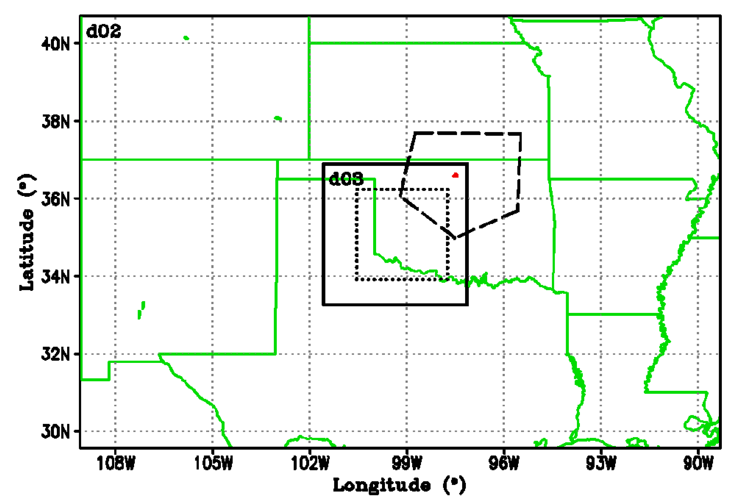
In this paper, we used the Weather Research and Forecasting model (WRF, version 3.5.1) to simulate the squall line on 20 May 2011 over the SGP. The WRF two-way nesting technique was used and the three-nested grid meshes had 171 × 131 × 61, 321 × 226 × 61 and 381 × 381 × 61 grid points with 25 km, 5 km, and 1 km horizontal resolution and time steps of 25 s, 5 s, and 1 s, respectively.
Figure 1 shows the middle and innermost model grid configuration. The central facility (Lamont, OK, USA) during the MC3E was located at the northeastern corner of the innermost domain and to the northeast of the largest subdomain with the size of 256 km.
The Goddard GCE microphysics scheme [
26] was used for the grid-resolvable cloud and precipitation parameterization. The Goddard long-wave and shortwave radiation parameterization [
27,
28] was employed for the radiative flux calculation and its interaction with microphysical processes. The Mellor-Yamada-Janjic (Eta) TKE scheme [
29] was used to represent the planetary boundary layer (PBL) sub-grid scale physical processes. The surface process employed the Monin-Obukhov (Janjic Eta) scheme [
29,
30] and the Unified Noah Land-surface model [
31] to calculate the surface fluxes over the ocean and land, respectively. The Grell-Devenyi scheme [
32] was used for convective parameterization for the 2 outer domains (25 km and 5 km). We used the finest resolution WRF as a CRM to explicitly simulate the convective behavior and its interaction with large-scale forcing.
The 0.5° × 0.5° horizontal resolution Global Forecast System (GFS) analysis data were used as the initial and lateral boundary conditions for the outermost domain at 6 h intervals. The inner domains (5 km and 1 km) were provided with lateral boundary condition through interpolation from the outer domains (5 km and 25 km). This GFS dataset had 26 pressure levels up to 10 hPa. The model simulation was initialized at 00 UTC on 20 May 2011 and was integrated for up to 18 h, which covered the generation and development stages of the squall line [
25].
The synoptic condition of the background state for the squall line system was described in [
25] and [
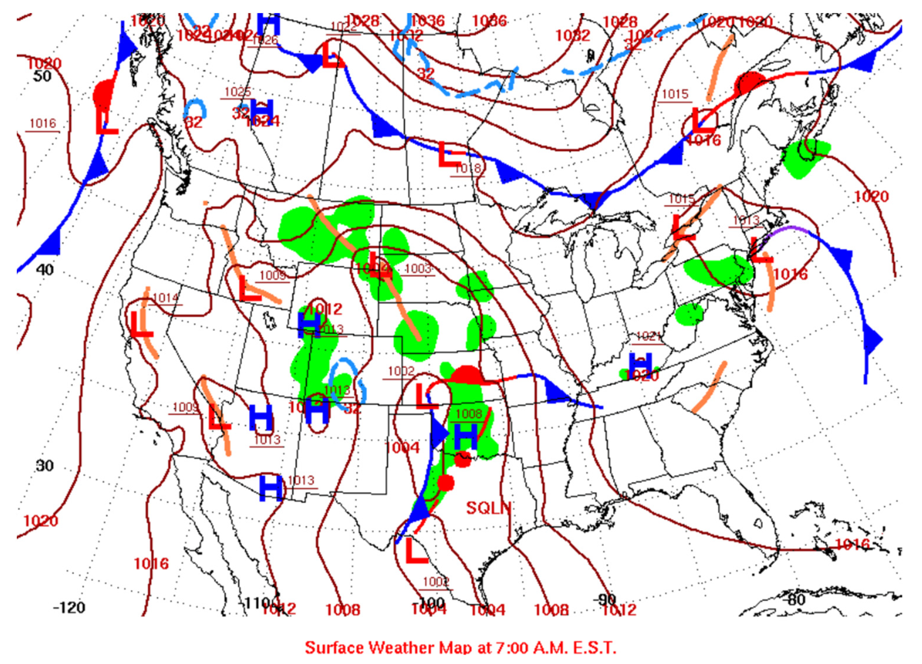
21]. It had an upper-level trough, a dry line, and a low-level warm and moist flow, all favorable for convection development. On 19 May 2011, a north-south oriented upper level trough formed over the Great Basin. In front of the trough, a dry line was located in the western Oklahoma panhandle, and east of the dry line a low-level, southerly warm and moist Gulf flow was located over central to eastern Texas and Oklahoma. A broken line of supercell thunderstorms initially developed along the dry line in the afternoon and evening of 19 May and then moved slowly northward. As the eastward-moving trough axis went further into New Mexico and Colorado in the morning of 20 May, the surface weather map showed a strong low pressure center elongated in the north-south direction across Texas, Oklahoma, and Kansas (
Figure 2). The upper level trough coupled with the northward-moving convection and a continuing south-southeasterly low-level warm moist flow ahead of the trough created a large quasi-linear meso-scale convective system (MCS), which developed and propagated across the MC3E experimental area. The interaction between the strong convective system and large-scale forcing led to intense convective precipitation and broad stratiform precipitation.
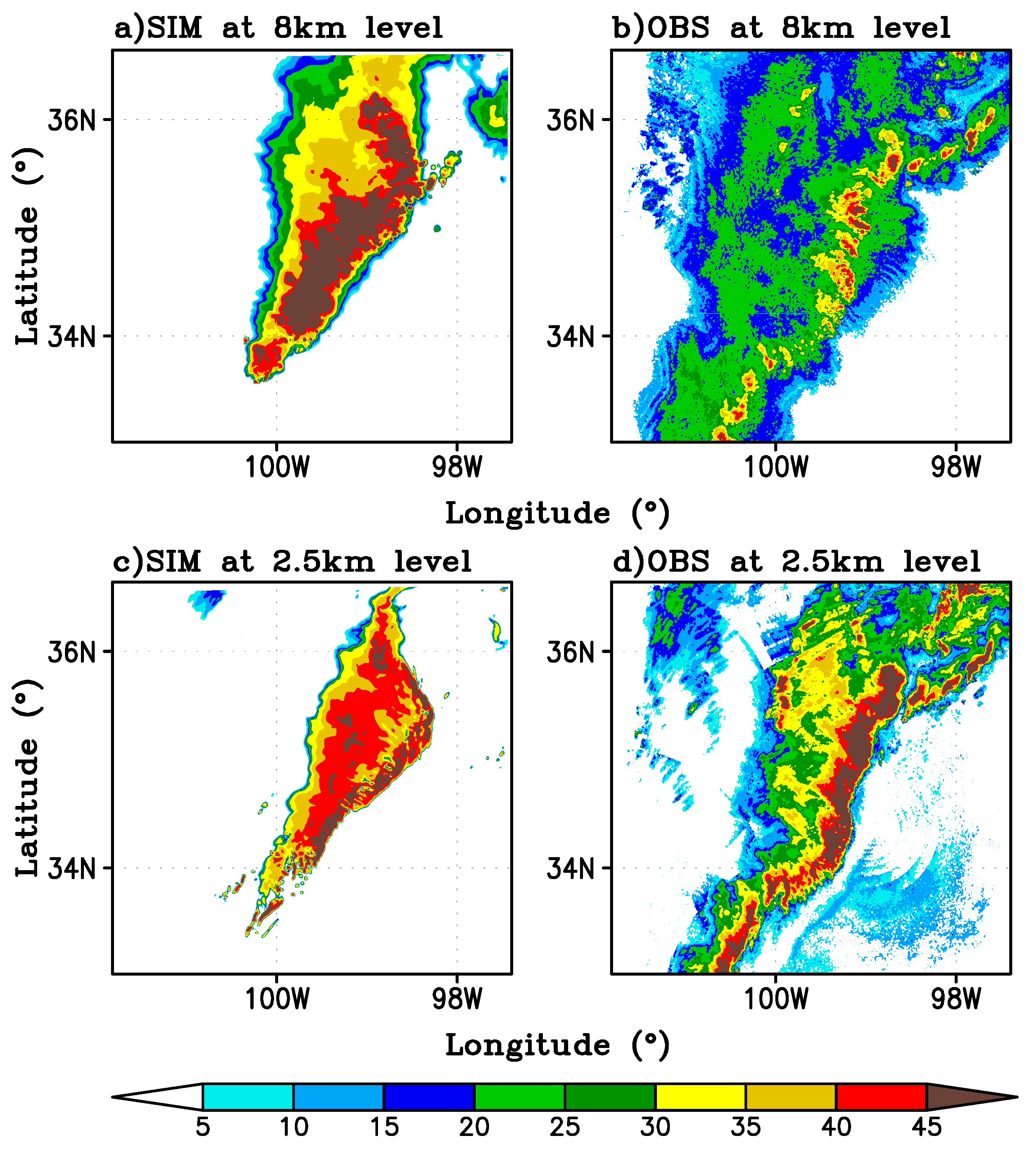
The CRM-simulated and observed radar reflectivity are shown in
Figure 3. The model captured some observed features of the squall line, such as its peak intensity and distribution at 8 km and 2.5 km altitudes. Both the modeled and observed strong echoes of the squall line (the area with reflectivity greater than 45 dBZ) were mostly found from 98 to 100° W and 34 to 36° N, extending from northeast to southwest. Moreover, the peak values of radar reflectivity from both the model and observations mainly appeared in the front edge of the squall line. It should be noted, however, that the WRF simulated reflectivity has weaker intensity than the observed one in areas to the east of 98 °W and to the west of 100 °W, especially at 2.5 km.
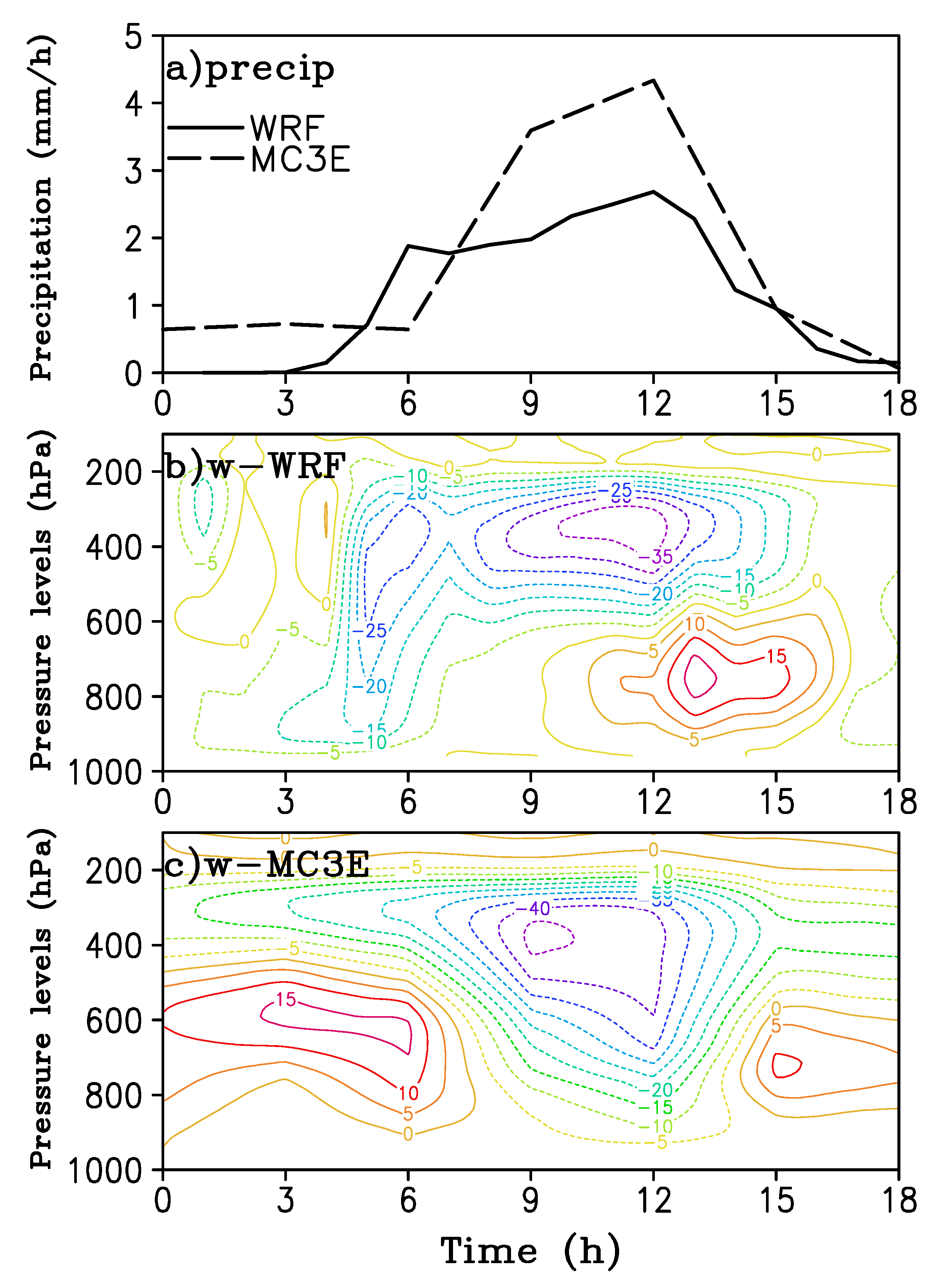
The simulation was verified against 300 km MC3E analysis forcing data (
Figure 4). Here, the WRF simulation data were averaged over the area (99.5~95.5° W, 35–38° N), which was very close to the 300 km MC3E variational analysis domain. There was a good agreement in precipitation rate between the 5 km resolution WRF simulation and the MC3E analysis, but the simulated precipitation was weaker than observed. Furthermore, both the modeled and analyzed strong ascending motion were present between 300 hPa and 400 hPa after 09 UTC with peak values of about 35 hPa/h for simulation and 45 hPa/h for analysis. The noticeable downward motion occurred at lower levels after 12 UTC for WRF and after 14 UTC for analysis, with the model producing a stronger downward motion. However, there was a large difference in the vertical velocity pattern between the simulation and analysis during the first 6 h simulation period, probably due to model spin-up. The time series of 500 hPa vertical velocity from WRF simulation (not shown) after the first 6 h was comparable to that from MC3E except with weaker intensity, consistent with precipitation difference. The timing of observationally diagnosed and modeled vertical velocity was also different. The MC3E diagnosed vertical velocity reaches a maximum around 9 h, while the model simulated maximum upward motion occurred 2 to 3 h later. On the other hand, the low-level downward motion occurred too early in the model compared to the observations. Since the model simulated fields were self-consistent and not drastically different from observations, we did not expect these differences to affect our analysis systematically.
3. Analysis Method
As stated earlier, the CRM domain covered 381 km × 381 km horizontally. We chose a 256 km × 256 km subdomain in the interior of the CRM domain to analyze convective behavior and its interaction with large-scale forcing using the CRM simulation data for the period from 00 UTC to 12 UTC on 20 May 2011. The squall line was within this subdomain during its initial and development stages. Similar to the work in [
19], the WRF data over the 256 km × 256 km subdomain was divided into different-sized subdomains with grid spacing of 128 km, 64 km, 32 km, 16 km, 8 km, 4 km, and 2 km, respectively. The averages over each of these 7 subdomains were equivalent to the grid–scale variables at current and future GCM resolutions. Therefore, the relationships between convective activity and a corresponding subdomain mean thermodynamic variable measured how well the latter could be used as a closure variable as GCM model resolution changes.
The CRM convective precipitation averaged over a subdomain represented the collective behavior of convection for the corresponding subdomain. The convective precipitation rate was the sum of the precipitation rate at convective grid points divided by the whole subdomain area. Following Xu and Randall [
34] and Suhas and Zhang [
19], a grid point was defined convective if the vertical velocity was above 1 ms
−1 or below −1 ms
−1 and at the same time, the sum of mixing ratio of cloud water and ice was greater than 1 × 10
−5 kg/kg.
The convective mass flux was often used as another measure of convection. It was defined using the following equation,
where
M is the mass flux,
σ is the fractional area coverage for convection,
ρ is air density and
w is vertical velocity averaged over convective grid points.
For large-scale variables, the vertical velocity at pressure levels is directly calculated through interpolation from the CRM-predicted vertical velocity at sigma levels. The vertically-integrated moisture convergence is defined as
where
is 3-D wind vector, representing the zonal, meridional, and vertical components of the wind,
q is the mixing ratio of water vapor,
g is acceleration due to gravity, and
ps is the lowest model level pressure. Note that the mass continuity equation has been used in Equation (2) to convert moisture convergence from flux form to advection form. We add a negative sign in front of the integral thus that positive values represent moisture convergence. It should be noted that for the 256 km and 128 km subdomains, the large-scale horizontal moisture convergence cannot be calculated directly using finite difference due to the insufficient number of subdomains. Thus, we employ Green’s theorem and convert the calculation of horizontal moisture convergence from the surface integral form to the line integral form.
Finally, the large-scale rate of change of CAPE in the troposphere above the PBL from time step
t to
t +δt is calculated by
where
is the environmental virtual temperature,
is the environmental virtual temperature after the large-scale advection above the PBL is applied,
R is gas constant, and
pb and
pt are pressure values at the parcel lifting level and the neutral buoyancy level, respectively.
4. Relationship between Precipitation and Large-Scale Forcing Using MC3E Data
The MC3E single column model forcing dataset (version 2) over the 300 km analysis domain throughout the entire analysis period from 00 UTC 22 April to 21 UTC 6 June 2011 was used to examine the relationship between the large-scale forcing and precipitation. We focused on large-scale CAPE change (dCAPE), column integrated moisture convergence, and 500 hPa vertical velocity. dCAPE was defined as the difference of CAPE values after and before the 3D large-scale advection of temperature and moisture was applied to temperature and moisture fields. dCAPE was found to be well correlated with convection at the Southern Great Plains [
8]. Moisture convergence had been used as a closure for convection in convection schemes [
12,
14]. The vertical velocity at 500 hPa had been used to describe large-scale circulation regime in studies of climate, clouds, and GCM model biases [
35,
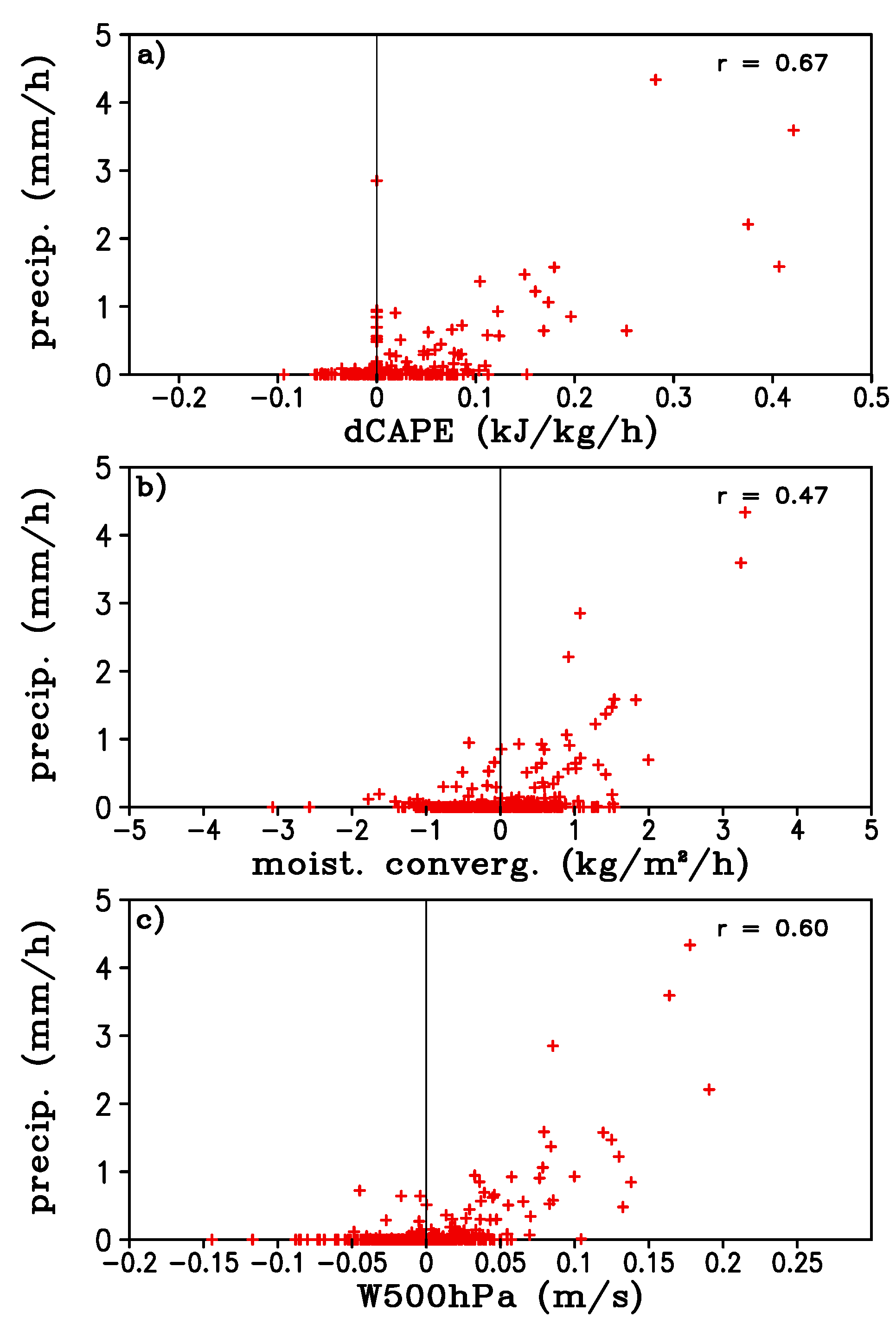
36]. In addition, advection of dry static energy and moisture by vertical velocity constituted an important part of both dCAPE and moisture convergence. The scatter plots of precipitation rate as a function of the 3 large-scale variables across 300 km analysis domain are shown in
Figure 5. The precipitation was fairly well correlated with dCAPE, and 500 hPa vertical velocity, with correlation coefficients of 0.67 and 0.60, respectively, (
Figure 5a,c). The moisture convergence had a relatively lower correlation with precipitation, with a correlation coefficient of 0.47 (
Figure 5b). This may be partly due to the fact that in some convective events moisture convergence is in phase with precipitation and in other convective events moisture convergence leads precipitation [
24]. In general, there was a good correspondence between precipitation and the 3 variables when there was heavy precipitation, meaning strong convection events. For the many non-precipitating or weak precipitation points the relationship is poor. Had we excluded the non-precipitating or weak (e.g., 0.5 mm/h) precipitation data points, the correlation coefficients would have been improved for moisture convergence and 500 hPa vertical velocity (0.73 and 0.67, respectively) but decreased for dCAPE (0.56).
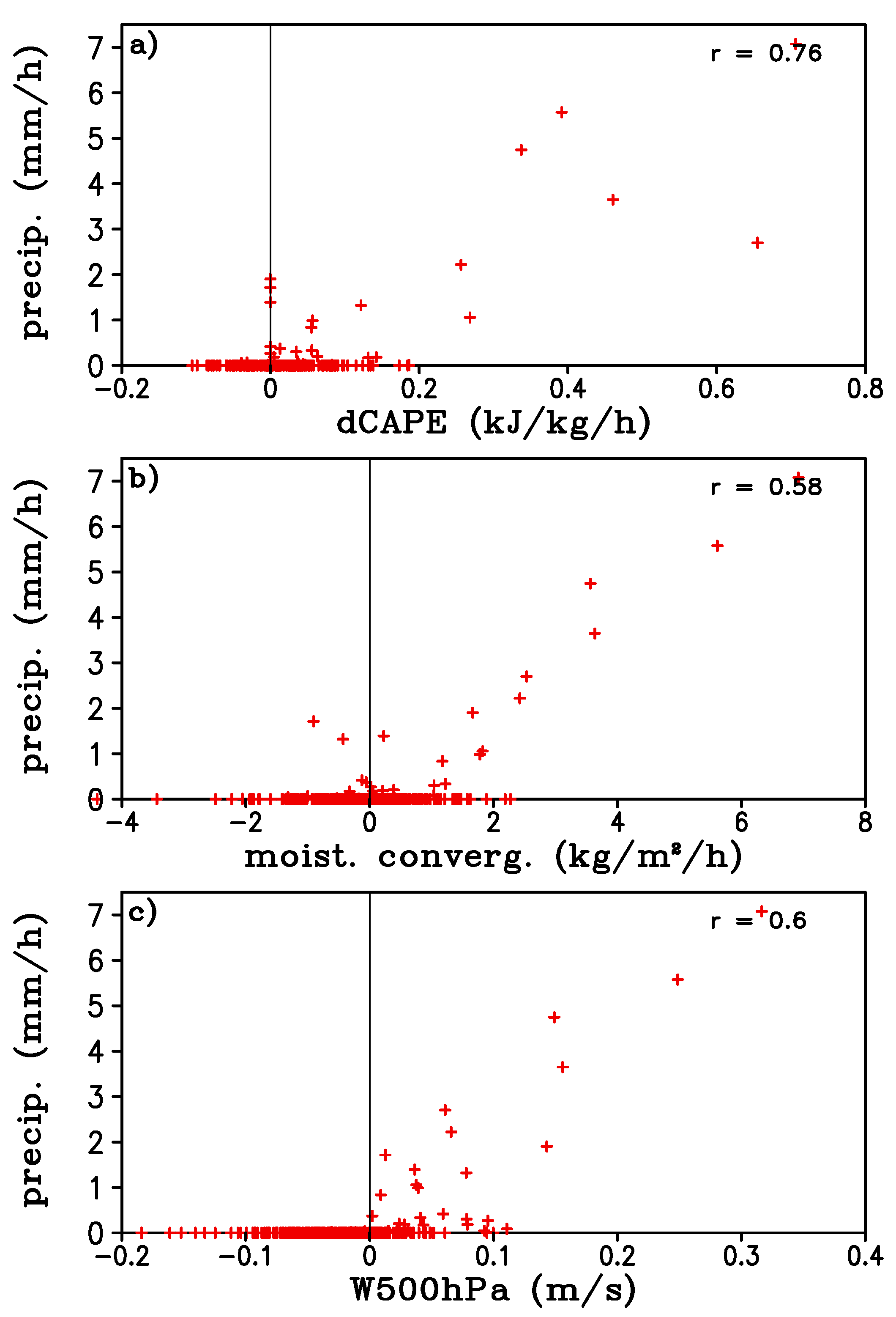
Figure 6 shows the same scatter plots as
Figure 5 but for the 75 km MC3E domain. The correlation was better between the large-scale variables and precipitation when the analysis domain size decreased from 300 km to 75 km, except 500 hPa vertical velocity, with correlation coefficients of 0.76, 0.58, and 0.6, respectively. Note that all data points were included in the calculation of correlation coefficients. If we had excluded the data points with negative large-scale variables, the relationship would have been improved significantly for both domains. For example, if only data with dCAPE > 0 were used, for the 300 km domain the correlation coefficients were increased to 0.74, 0.56, and 0.74 between precipitation and large-scale CAPE change, moisture convergence, and vertical velocity at 500 hPa, respectively.
5. Relationship between Convection and Large-Scale Forcing Using CRM Data
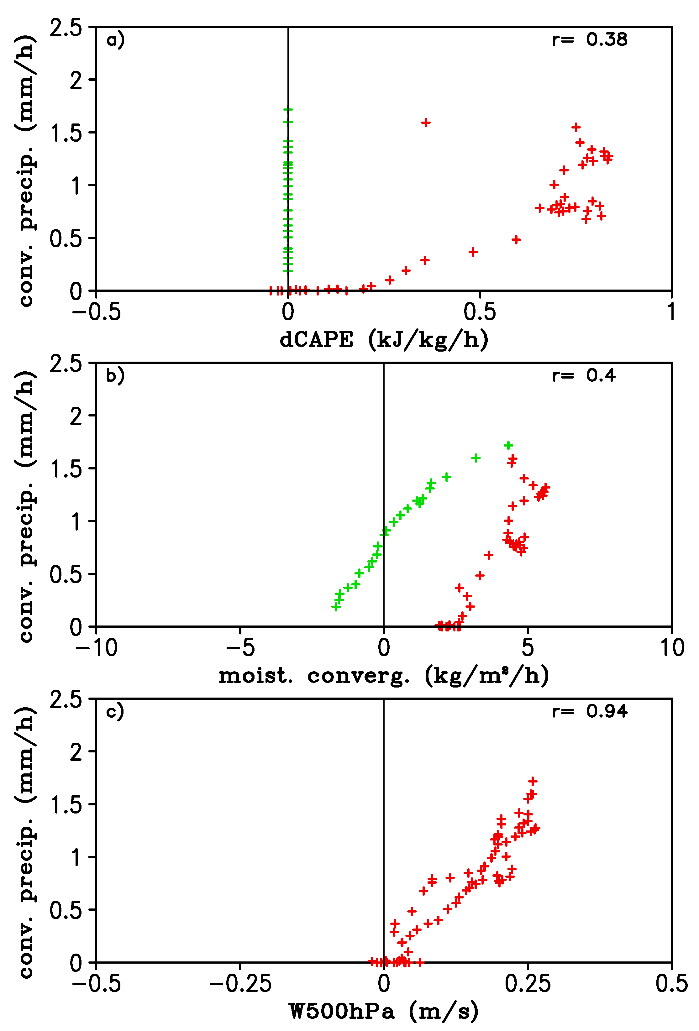
The 256 km subdomain was chosen first to examine the relationship of convective precipitation with large-scale forcing.
Figure 7 shows the scatter plots of convective precipitation rate as a function of large-scale variables. The 500 hPa vertical velocity has an excellent relationship with convective precipitation with a correlation coefficient of 0.94. On the other hand, the correlation between convective precipitation and moisture convergence or large-scale CAPE change was poor, with correlation coefficients of 0.4 and 0.38, respectively. This was largely caused by the separation between data points with dCAPE > 0 and those with dCAPE = 0. Note that in the calculation of dCAPE, it was set to zero if the atmosphere was convectively stable, that is, if CAPE = 0. If we excluded these convectively stable points, the correlation coefficients between convective precipitation and moisture convergence or large-scale CAPE change were much higher (0.93 and 0.87, respectively). The reason for the existence of these zero CAPE and/or dCAPE but large precipitation amount was that the atmospheric condition within this 256 km × 256 km domain was highly inhomogeneous. There were highly unstable sub-regions, in which convection occurred, as well as highly stable regions where there was no convection. The average atmospheric condition over the entire domain, however, was stable, leading to zero CAPE.
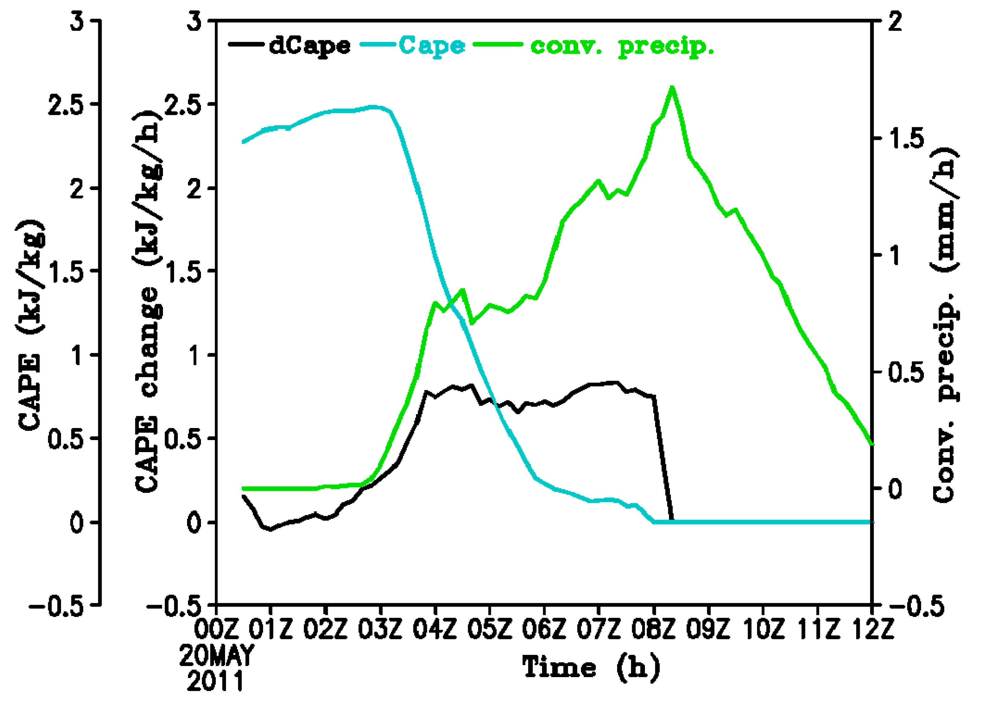
Figure 8 shows the time series of domain-averaged CAPE, dCAPE and convective precipitation rate. There was a large amount of CAPE, which continued to build up prior to 03 UTC, but there was little convective precipitation or dCAPE. After 03 UTC, CAPE dropped rapidly as precipitation picks up and dCAPE increased. From 03 UTC to 07 UTC, convective precipitation in general increased with dCAPE. After 08 UTC, dCAPE was zero due to stable mean atmospheric condition (CAPE = 0) and remained zero until 12 UTC, but at the same time convective precipitation decreased almost linearly from the peak value to about 0.2 mm/h.
Figure 9 shows the same plots as
Figure 7, except for 128 km subdomain averages. All large-scale variables have good relationships with convective precipitation. The correlation coefficients involving vertical velocity at 500 hPa, moisture convergence, and dCAPE were 0.89, 0.75, and 0.78, respectively. There were still points with dCAPE = 0. However, due to the small number of them, they did not affect the correlation coefficient as much as in
Figure 7. Excluding these points, the correlation coefficients between convective precipitation and moisture convergence/dCAPE would have been 0.81/0.88.
Mass flux at the cloud base was often used as a measure of convective activity in convective parameterization closures. However, convection intensity can be associated with mass flux at any pressure level, at or above the cloud base [
15,
37]. Thus, we will first identify the pressure level at which mass flux can best measure convective intensity in terms of precipitation for the squall line simulation here.
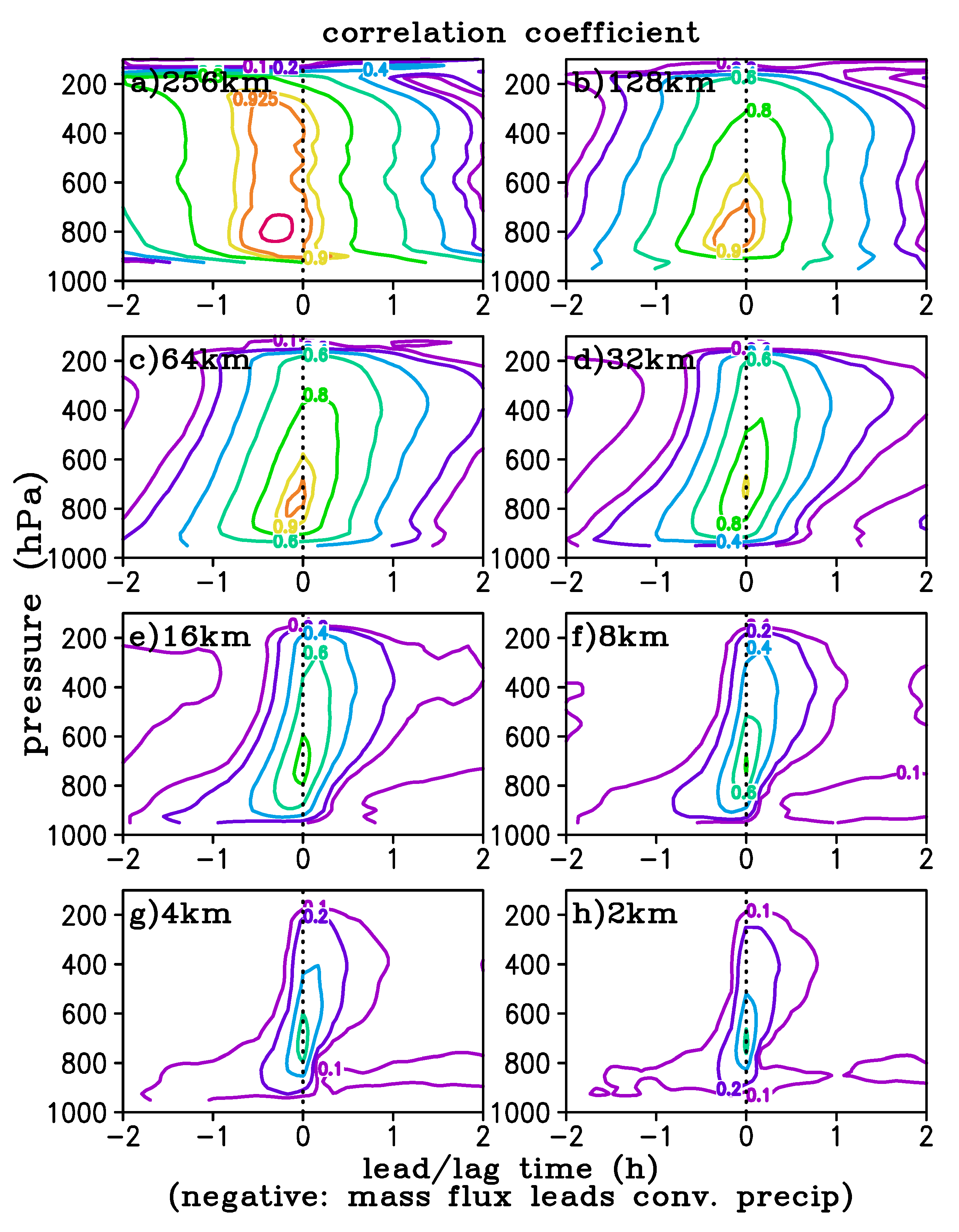
Figure 10 shows the lead-lag correlation between convective precipitation and mass flux at different pressure levels for various subdomain sizes. The maximum correlation coefficients are near 800 hPa for 128 km and 64 km subdomains when mass flux leads to convective precipitation by about 10 min and 5 min, respectively. For smaller subdomains (32 km, 16 km, 8 km, 4 km, and 2 km) the maximum correlation coefficients occurred around 700 hPa with no time lag between mass flux and convective precipitation. Furthermore, in the lower levels, the maximum correlation occurred when mass flux led convective precipitation, but in the upper levels, it occurred when mass flux lags convective precipitation. This was because convective clouds developed first in the lower troposphere, gradually moved up, and then precipitation began. After the mature stage when precipitation began to weaken, clouds continued to linger in the upper troposphere. This was similar to that found in tropical convection by Suhas and Zhang [
19]. The maximum correlation coefficients were the highest for the largest subdomain size, greater than 0.95 for 256 km subdomain, and decreased to 0.6 for the 2 km subdomain size. This means that for large-scale averages, convection in terms of convective mass flux is synonymous to convective precipitation. For convective scale (O(km)) when there is upward motion or convective mass flux, there may or may not be precipitation. This makes sense as precipitation often falls out of updrafts and coincides with downdrafts areas at convective scale.
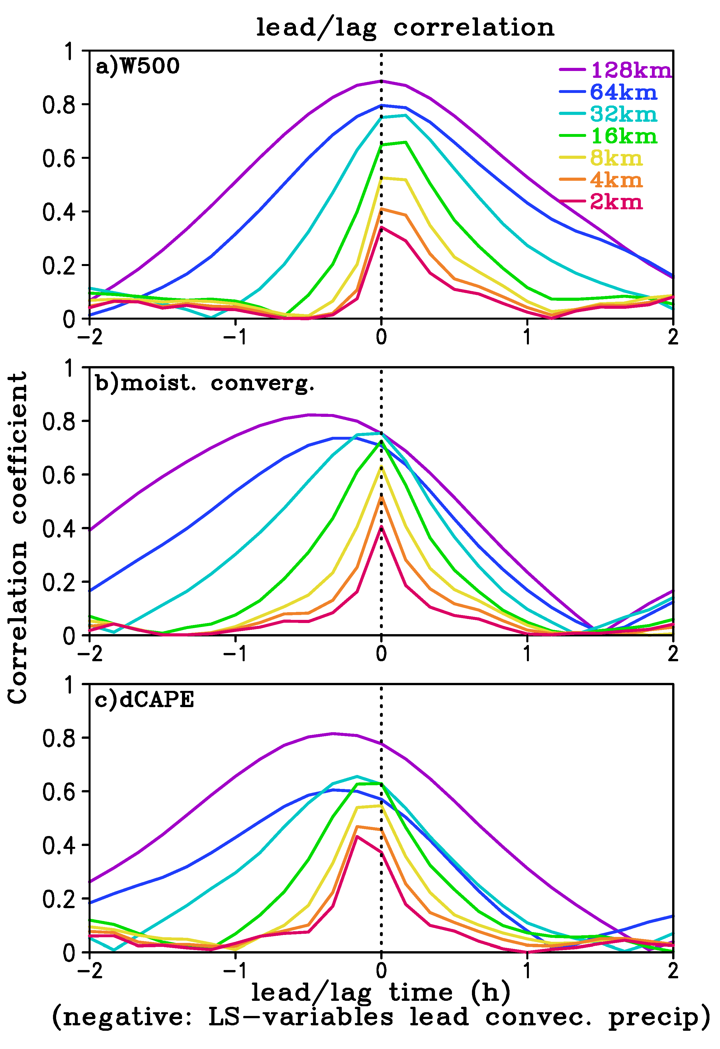
The lead-lag correlation between convection and large-scale forcing is shown in
Figure 11. The maximum correlation generally decreased with subdomain size for all variables. This was likely because the large-scale control of convection became weaker and other non-deterministic factors such as stochasticity became more important as the scale became smaller. The strongest relationship between convective precipitation and 500 hPa vertical velocity was found when they were nearly simultaneously correlated for various subdomains. However, there was a clear skew towards a positive lag, particularly for subdomains 32 km or smaller, that was, 500 hPa vertical velocity lags convective precipitation. This means for smaller subdomains vertical motion is to some extent a response to convective heating. The moisture convergence led convective precipitation for subdomains 32 km or larger. For smaller subdomains, there was little or no lead. The decreasing lead time for moisture convergence with decreasing subdomain size was similar to that found in tropical convection [
19]. The dCAPE showed largest correlation with convective precipitation when the former leads the latter by 20 min for 128 km and 64 km subdomains, and by about 10 min for the smaller subdomains. In general, dCAPE had the largest lead to precipitation, followed by moisture convergence, whereas the 500 hPa vertical velocity lags precipitation. For all three variables examined, the maximum correlation decreased greatly with decreasing subdomain size (
Table 1).
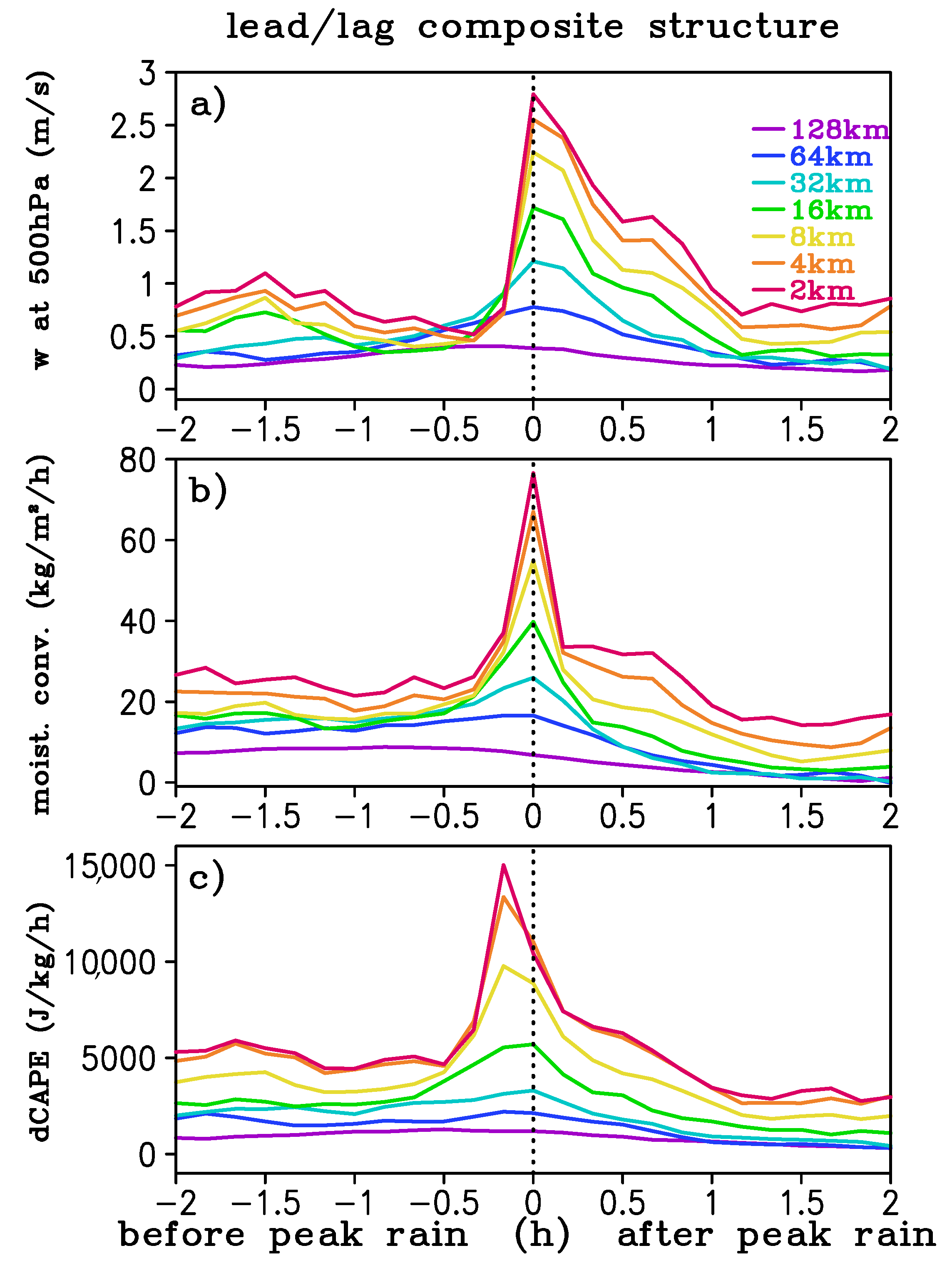
We next analyzed the lead/lag composite structure of large-scale variables (
Figure 12). It was found that the peaks of large-scale variables increased with decreasing subdomain size. This is because at smaller scales vertical velocity has larger values. The associated fields such as column moisture convergence and CAPE generation by the grid–scale circulation were also larger. In addition, the lead time corresponding to the maxima of large-scale variables was generally consistent with that corresponding to the strongest correlation of large-scale fields with convection. For subdomains smaller than 64 km, the large-scale atmosphere exhibited relatively small dCAPE, weak moisture convergence and weak vertical velocity half an hour prior to the peak convective precipitation, and then large-scale forcing started to strengthen greatly. First, dCAPE reached the maximum rapidly and about 10 min later moisture convergence and vertical velocity at 500 hPa peaked at the same time as that for the peak convective precipitation. This was different from the investigation by Suhas and Zhang [
19], who found that the maximum moisture convergence appeared 16–30 min before the peak precipitation for subdomains from 4 km to 64 km. After the peak time, large-scale variables decreased sharply, especially when the subdomain size was smaller than 16 km. Nevertheless, there was a clear asymmetry before and after the peak of each variable; they decreased more slowly than they increased before reaching the peak, especially for 500 hPa vertical velocity.
6. Summary and Conclusions
In this study, the WRF model is used to simulate a squall line observed on 20 May 2011 in the Southern Great Plains of the United States. The 1 km resolution CRM simulation data are spatially averaged to represent the GCM grid spacings of 128 km, 64 km, 32 km, 16 km, 8 km, 4 km, and 2 km. Then we evaluate the relationship of convection over mid-latitude with mass flux and large-scale variables using the CRM simulation data.
We examine the relationship of mass flux with convective precipitation and find that the maximum correlation coefficients between them are mainly between 800 hPa and 700 hPa when mass flux leads convective precipitation about 5~10 min for 128 km and 64 km subdomains or when they are simultaneously correlated for smaller subdomains. Hence, the vertical level at which mass flux best measures convection for most GCM horizontal resolutions is lower than that for tropical oceanic convection (600 hPa) found in the work of [
19]. Good relationships (~0.6) are found in the whole troposphere when the subdomain sizes are greater than 16 km, and the correlation remains high (~0.6) between 600 and 800 hPa when the subdomain sizes decrease to 8 km or smaller. Additionally, the lead time/lag time between mass flux and convective precipitation is longer/shorter at lower levels than that at upper levels, indicating that deep convection develops from the shallow convective system and dissipate from lower levels.
The relationship between convection and GCM grid–scale forcing at various subdomain sizes is also examined. The strongest relationship of convective precipitation with the vertical velocity at 500 hPa is found when they are nearly simultaneously correlated for various subdomains and the correlation decreases with decreasing subdomain size. Both the maximum correlation of convection with moisture convergence and large-scale CAPE change and the lead time corresponding to the largest correlation decrease with decreasing subdomain size.
The lead/lag composite analysis on large-scale forcing indicates that peaks of large-scale variables increase with decreasing subdomain size and the lead time corresponding to the maxima of large-scale variables is consistent with that corresponding to the strongest correlation of large-scale fields with convection. Different from the investigation by Suhas and Zhang [
19], the maximum moisture convergence is reached at the same time as that for the peak convective precipitation for subdomains smaller than 64 km.
The analysis on lead/lag correlation and lead/lag composite structure indicates that convection responds to the large-scale CAPE change for a wide range of horizontal resolutions. Except for 128 km and 64 km, moisture convergence occurs at the same time with convective precipitation. The vertical velocity is likely a result of convection. Thus, the large-scale CAPE change seems to be a better closure variable for convective parameterization between those three large-scale fields.
The relationships between convection and equivalent GCM grid–scale variables examined in this study is based on a cloud-resolving model simulation of a midlatitude squall line. Compared to Suhas and Zhang (2015), which used cloud-resolving model simulations of six days of unorganized convection during the break monsoon period in Australia, we only have a single convection case. Thus, it is not clear whether they apply to other convective systems or unorganized convection in the midlatitude convective environment. Further studies of more cases are needed to reach a firmer conclusion.


