1. Introduction
A main concern of scientists and forecasters alike is the identification of atmospheric vortices and the analysis of their potential impact. The most common example is the local impact of synoptic-scale low-pressure systems. It is a difficult task to analyze these vortices since multiple scales are involved. To understand the vortex interactions between these scales, we need differently-resolved datasets. However, a single method of vortex identification, which is independent of the data resolution, is missing so far. Moreover, existing meteorological methods usually fail to identify the vertical structure of a vortex in a consistent manner. In this work, we will present a kinematic method (-method) that satisfies these two requirements. It unifies existing methods and can be applied to differently-resolved datasets. Additionally, it does not need height-dependent adjustments, allowing for a three-dimensional analysis of atmospheric phenomena.
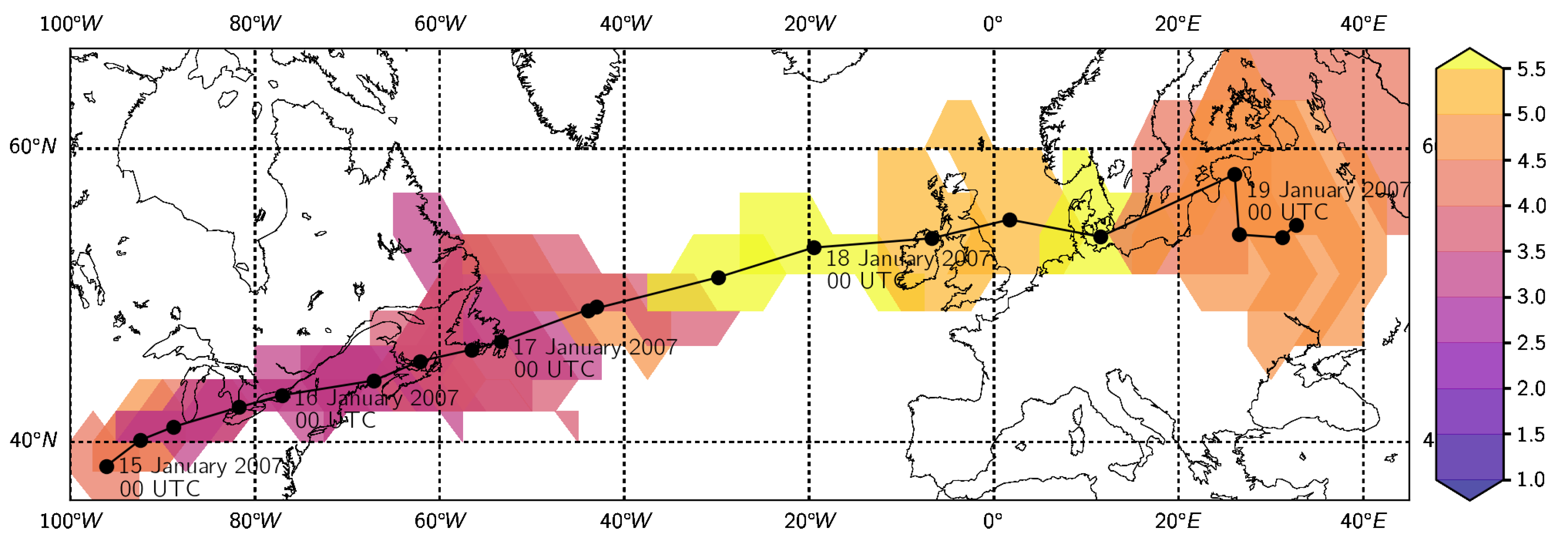
In this work, we will demonstrate the strength of this vortex identification method and apply it to the complex weather event caused by a cold-season high-impact extratropical cyclone. We chose winter storm Kyrill, which caused high damage across Europe on 18 January 2007. The event was well forecast, and hence, we expect the models to mirror properly the various aspects of Kyrill. Due to its high impact, this cyclone has been the subject of studies in the past. This allows us to address the characteristics of the event and compare our method with previously-published results. High-resolution model data could be made available for our purpose due to this reason as well. Moreover, the local impact of Kyrill was characterized by various phenomena of different scales. In particular, convective storms embedded in the larger-scale vortex had a large influence on the local intensity of the event. Therefore, this storm system is a challenging situation for a vortex identification method. Moreover, we think that our results are of interest to a broad audience including scientists, teachers, and forecasters.
Though it seems to be obvious what a vortex is, the identification of its intensity and size is a non-trivial task. The main problem is that a clear (mathematical) definition of a vortex [
1] or of an extratropical cyclone [
2] is still lacking. Regarding extratropical cyclones, commonly-used intensity measures are either based on the search for local minima in the pressure or geopotential height fields, e.g., [
3,
4], or local maxima of the (geostrophic) vorticity, e.g., [
5,
6]. The area of extratropical cyclones can then be estimated by closed contours around the inspected fields such as closed isobars as in [
3] or by fixed thresholds as, e.g., in [
7]. Concerning the impact of a storm, another useful intensity measure is the wind speed above a fixed wind magnitude or above a certain percentile, e.g., [
8]. Though, this detects the wind-affected regions associated with the storm rather than the vortex itself.
However, these traditional meteorological methods have some drawbacks: Pressure-based identification methods of vortex intensity and size can fail when the cyclones are embedded in strong constant background flows [
6]. Moreover, when a cyclone moves into a region of lower background pressure, pressure tendencies at the vortex center can falsely indicate an intensification [
9]. Local vorticity extrema do not take into account the vortex size. Hence, the impact of the system can be misjudged (e.g., Sinclair [
9] gave examples of systems with similar local vorticity extrema, but one was small, the other large). Additionally, methods based on vorticity thresholds can be misleading when the vortex is embedded in an environment of shear [
1]. Since shear is a prominent feature of atmospheric flows, in particular in the upper troposphere, threshold-based methods need adjustments or can fail completely (e.g., see Figure 12 in [
10]). It is then unclear if the same part of the vortex was identified throughout different height levels. Moreover, vorticity depends on the spatial scale of the data and has a smaller scale than pressure, cf. [
5,
11,
12]. Hence, the higher the spatial resolution of the data, the more (smaller-scale) systems will be identified. This might be a disadvantage when one is interested in the study of synoptic-scale vortices.
Instead of local vortex intensity measures, global ones such as the circulation can be used [
9]. Circulation takes into account both the rotation of a vortex, as well as its size. The circulation is an important, necessary intensity measure for the study of the dynamics of a set of point vortices for example. Though point vortices are a highly-idealized model of a vortex under barotropic, inviscid, incompressible conditions, they can be used to describe synoptic-scale vortex motions and can, e.g., explain the (quasi-)stationarity of blocking [
13,
14]. Moreover, under inviscid, incompressible conditions, Kelvin’s circulation theorem states that the absolute circulation is a conserved quantity. Due to its dependence on size, the main challenge in estimating the circulation remains since vortex
size identification based on pressure or vorticity suffers from the same drawbacks as the already mentioned methods.
In order to avoid these drawbacks, kinematic methods can be used. Kinematic methods are often based on the velocity gradient tensor
and its invariants. Since the methods are based on gradients of the wind field, constant background flows do not affect the identification as in pressure-based methods. The velocity gradient tensor
can be expressed as sum of the symmetric strain-rate tensor
and the skew-symmetric rotation tensor
. A comparison of these rotational and deformational flow properties helps to differentiate between vorticity caused by a shearing motion or by a real vortex. Some examples of kinematic vortex identification methods are the
-method [
1], the
Q-method [
15], the
-method [
16], the Okubo–Weiss parameter [
17,
18], and the kinematic vorticity number
[
19,
20]. Most of the methods compare the skew-symmetric rotational parts related to the vorticity tensor
to the symmetric deformational parts expressed by the strain-rate tensor
S. If at all, the methods only differ in the amount of the rotation necessary in comparison to the deformation in order to define a vortex [
21]. The
Q-method, Okubo–Weiss parameter, and kinematic vorticity number
are even directly related. Despite their advantages and though their number is increasing, kinematic methods have to date only been applied in a few, mainly sub-synoptic, meteorological studies: e.g., Dunkerton et al. [
22] and Tory et al. [
23] used the Okubo–Weiss parameter in the identification of tropical cyclones; Markowski et al. [
24] used the Okubo–Weiss parameter to identify vortices in convective-scale storms; Schielicke et al. [
10] used the
-method based on the kinematic vorticity number to identify synoptic-scale cyclones; and Schielicke [
25] studied vortices in differently-resolved datasets. However, a single system has never been studied by the same method throughout different scales so far.
With the help of the kinematic
-method, we will analyze the extratropical cyclone
Kyrill that crossed western and central Europe on 18 and 19 January 2007. Kyrill ranks first among the most devastating winter storms in Europe, causing 49 fatalities and an estimated total economic loss of 10 billion Euros [
26]. It exceeded other storm events with respect to the area affected by extremely high winds [
27]. It was associated with a convectively-induced wide-spread high-wind event: a cold-season derecho [
28]. Moreover, Fink et al. [
27] and Ludwig et al. [
29] described additional features of Kyrill that will be also addressed in our work. These are high winds close to the low-pressure center of Kyrill and the secondary cyclogenesis during the development of the cyclone. These aspects, and in particular the severe convective wind event embedded in the large-scale extratropical cyclone, will serve as a suitable system to test the ability of the
-method in identifying vortex structures and their properties among different scales. In particular, we will address the following research questions:
Is it possible to use a single method to detect the vortex structures embedded in the extratropical storm system Kyrill?
How does an increase in resolution affect Kyrill regarding vortex intensity and size throughout the depth of the troposphere? Will we observe an ensemble of smaller-scale vortices that form the larger-scale system?
Due to Kelvin’s circulation theorem, we expect that the intensity of these smaller-scale vortices in their sum is of comparable order to the intensity observed in coarser data. Can we confirm this hypothesis?
Is the size of the vortices reduced evenly with increasing resolution since the vorticity is a scale-dependent variable?
Moreover, we would like to test which intensity measures best visualize the impact of a vortex and if these measures are affected by the scale of the data. The paper is organized as follows: In
Section 2, we will briefly describe the different datasets used for the analysis. The vortex identification method (
-method) and the derivation of vortex properties derived with the help of the
-method are introduced in
Section 3. Our results will be presented and discussed in
Section 4. Finally, conclusions are given in
Section 5.
3. Methods
The vortex identification based on the kinematic vorticity number (
-method) and the derivation of vortex properties presented in
Section 3.1 and
Section 3.2 follows and builds on the work of Schielicke et al. (2016) [
10] and Schielicke (2017) [
25]. The methods described in
Section 3.3 and
Section 3.4 were computed with Python. The Python code can be requested from the authors. All plots have been produced with the python modules matplotlib, version 2.0.0, [
35] and the Basemap Matplotlib Toolkit, version 1.0.7, [
36]. Basemap uses cartographic material (e.g., coastlines) of the Global Self-consistent, Hierarchical, High-resolution Geography (GSHHG) Database [
37] (cf.
https://www.soest.hawaii.edu/pwessel/gshhg/ for more details) that is published under the GNU Lesser General Public License (
http://www.gnu.org/licenses/lgpl-3.0.html).
3.1. Vortex Identification
The velocity field
in the vicinity of a point
at time
t can be described by a (first-order) Taylor series expansion [
38,
39]:
The first term on the right-hand side is the uniform translation given by the velocity at the location of interest. The second term on the right-hand side includes the velocity gradient tensor
with
. This tensor is given by the derivatives of the velocity components
with respect to the space coordinates
. Explicitly, we have:
The velocity gradient tensor can be evaluated at every point in the flow field, and it describes the rotational and deformational parts of the flow. It can be decomposed into the symmetric strain-rate tensor
and the antisymmetric rotation tensor
, respectively:
where the superscript
stands for transpose, and
.
Following [
19,
20], we used the magnitudes, i.e., the tensor norms, of the strain-rate and rotation tensors in order to define rotation-prevailing regions of the flow. Truesdell [
19,
20] introduced the kinematic vorticity number
as the ratio of the local rotation rate and local strain-rate:
The kinematic vorticity number
is a dimensionless number. We can differentiate between three cases:
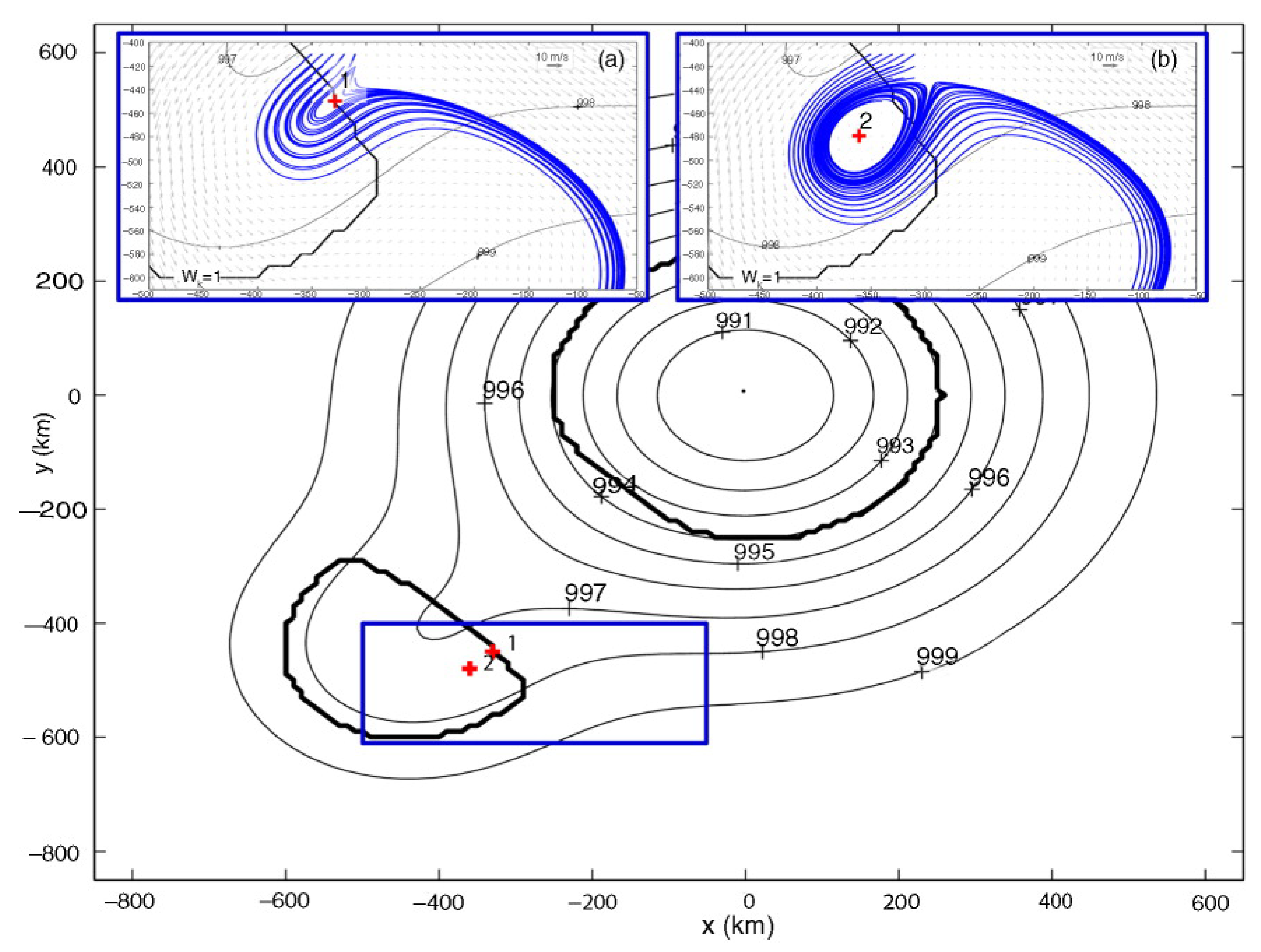
In this work, we define a vortex (core) as a simply-connected region of kinematic vorticity number
above one (or slightly higher). In this case, the rotation-rate prevails over the deformation-rate. With respect to the meaning of the
threshold of one, Schielicke et al. [
10] gave an example of the flow patterns around two points with different values of
that is reprinted in
Figure 1. Indeed, the local streamlines around Point 1 at the vortex boundary defined by
resemble a shearing flow. Though the streamlines curve around Point 1 at a farther distance, they are not trapped around Point 1 and do not stay close to it (
Figure 1, top left). On the other hand, streamlines close to Point 2 inside the vortex core with
spiral around and remain close to that point (
Figure 1, top right). Moreover, the work in [
10] pointed out that the threshold of
was connected to the vortex core. This means that the impact-related wind field associated with the vortex can be outside that core.
Local strain-rates and rotation-rates are calculated by the tensor norms of strain-rate and rotation tensor:
where
stands for the trace and the indices
symbolize the components of the tensor with
for 2D and
for 3D, respectively. In 3D, the symmetric strain-rate tensor has six independent components, and the antisymmetric rotation tensor has three independent components that are given by the components of the vorticity vector
. In 2D, the strain-rate tensor has three independent components
, while the rotation tensor is completely described by one independent component: the vertical vorticity
. Hence, we can calculate the kinematic vorticity number at every data point in 2D and 3d, respectively, as:
By taking into account the sign of the vorticity in , we are able to differentiate between cyclonically- and anticyclonically-rotating vortices. Furthermore, by using the 2D version of the kinematic vorticity number (), we implicitly assumed that the vortices rotated around a vertically-oriented axis. This is mostly true for larger-scale vortices. In this work, we mostly used the 2D version of the -method and will from now on drop the index (2D) in these cases. Whenever it is used, we will explicitly indicate the 3D version as -method.
3.2. Definitions of Vortex Properties
A vortex can roughly be seen as a three-dimensional rotating structure. Since a clear (mathematical) vortex definition is still lacking [
1], its properties are not properly defined. However, from idealized vortex models such as the Rankine vortex, we can deduce at least two important properties that determine the wind field around the vortex. These two properties are the circulation and the vortex radius. Though such vortex models are derived under idealized conditions, they represent an exact solution of the Navier–Stokes equations and can hence be interpreted as the highly-idealized version of a real vortex. For example, the axisymmetric Rankine vortex model is an exact stretch-free solution of the Navier–Stokes equations under incompressible, adiabatic, and inviscid conditions.
Let
A be the area of a vortex. By assuming that the identified area
A is equal to a circle
around the rotation axis of the vortex, we can determine an effective radius
by:
The circulation
of a vortex is given by:
where
is the velocity along the line
C enclosing the vortex area
A. Applying Stokes’s theorem, we can also express
with the help of the vorticity vector
as:
where
is the vector normal to the vortex area
A. For vortices rotating around a vertical axis, the circulation reduces to the areal integral over vertical vorticity
:
Though the circulation is a useful intensity measure, its value can be misleading in terms of the local impact of a vortex. Imagine two axisymmetric vortices with axisymmetric wind fields that have the same circulation. However, one system is small, the other large. Then, from Equation (
11), we can conclude that the wind speed at the circumference of the smaller vortex must be much stronger than the wind speed around the larger vortex. Hence, we additionally used the following two more impact-related intensity measures: Under the assumption of an axisymmetric vortex, we can deduce mean values of velocity
from Equation (
11):
and vorticity
from Equation (
13), respectively:
3.3. Computation of Vortex Properties
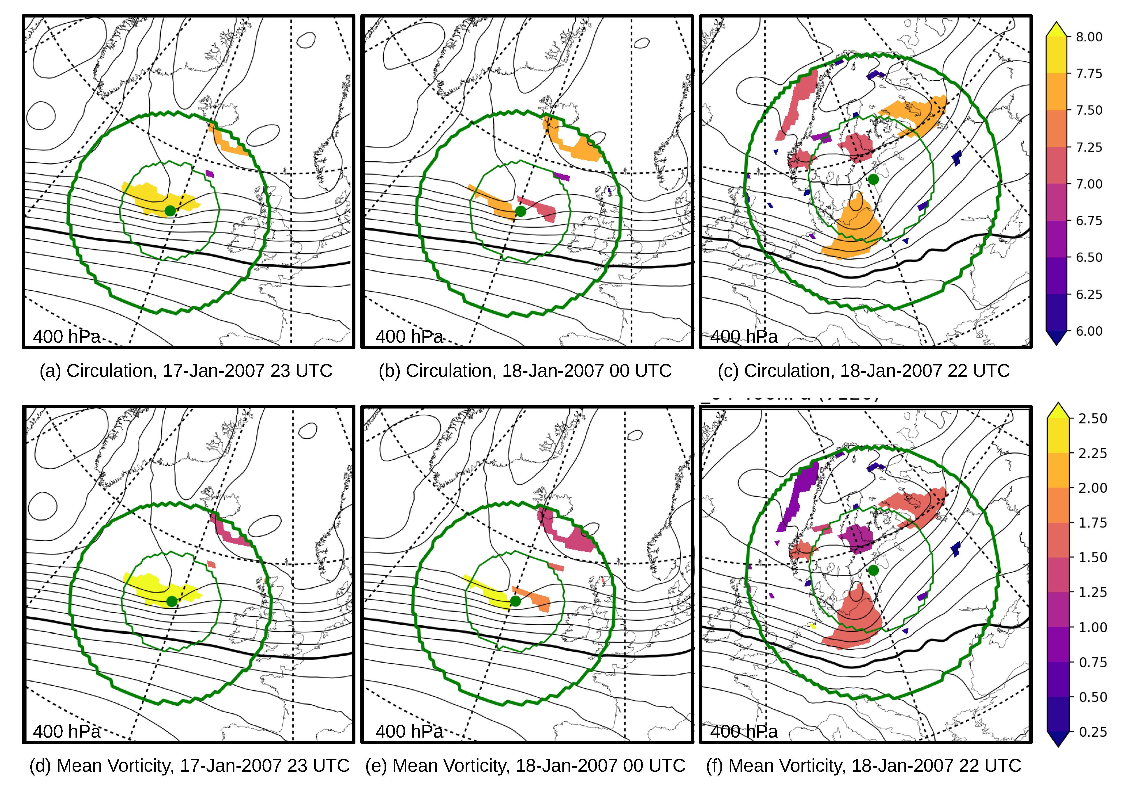
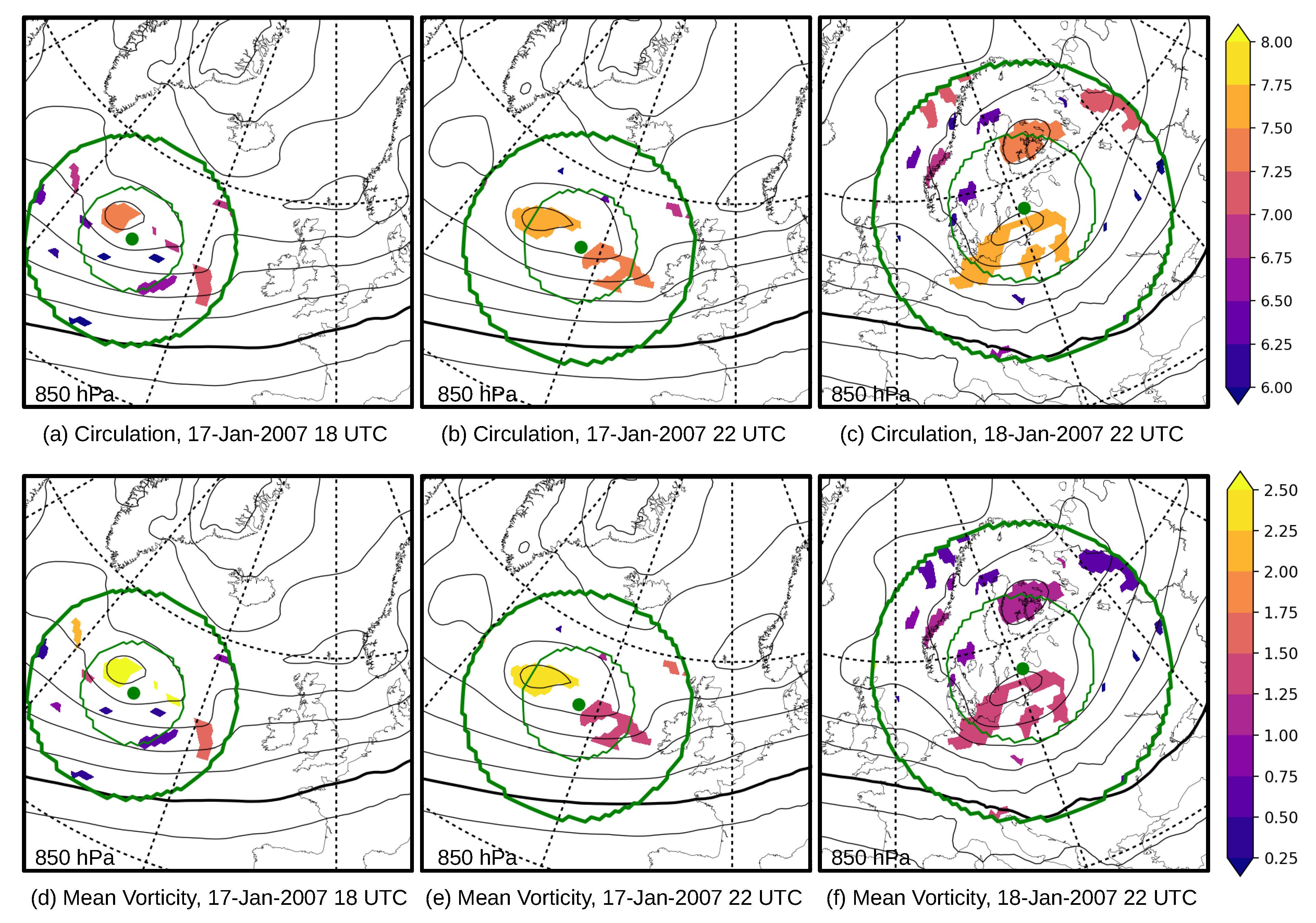
We used the -method in order to identify the size of a vortex given by the area associated with each simply-connected region of or a slightly higher threshold. Unless otherwise indicated, we used the two-dimensional -method. In order to derive a vortex patches field, we first calculated at every point in the field. Then, we set each point to one that had a larger than the threshold and each point with smaller than that threshold to zero. Note that these vortex patches fields can be multiplied with every other field of interest, e.g., multiplication with the field of the signs of vertical vorticity gave information about the orientation of the rotation (cyclonic, anticyclonic).
Each simply-connected vortex patch is associated with a certain number of grid points, and each grid point
i can be associated with an area
surrounding the point. The total
vortex areaA is then given by the sum of the areas associated with each grid point:
where
N is the number of grid points that belong to the vortex. Furthermore, each grid point
i is associated with a
circulation that is calculated by the vorticity
times the area
of the grid point. The total circulation of the vortex is then computed as the sum over all grid point circulations:
Moreover, we can calculate the
circulation center of a vortex by weighting the grid point coordinates
associated with the vortex by the circulation
at these points divided by the total circulation of the vortex as:
Kyrill’s circulation center derived from the coarsely-resolved NCEP data served as the central point of a circle of roughly 500–600 km. This region was then used to extract the vortex structures associated with Kyrill that we identified in the higher-resolved datasets.
3.4. Vertical and Temporal Tracking of Kyrill
In order to track Kyrill over time, we identified all cyclones with the help of the
-method using a threshold of
in the coarsely-resolve NCEP dataset as a first step. Then, we manually traced the cyclone at the lowest model level (1000 hPa) from 15 January–19 January 2007 18 UTC, according to the locations published in [
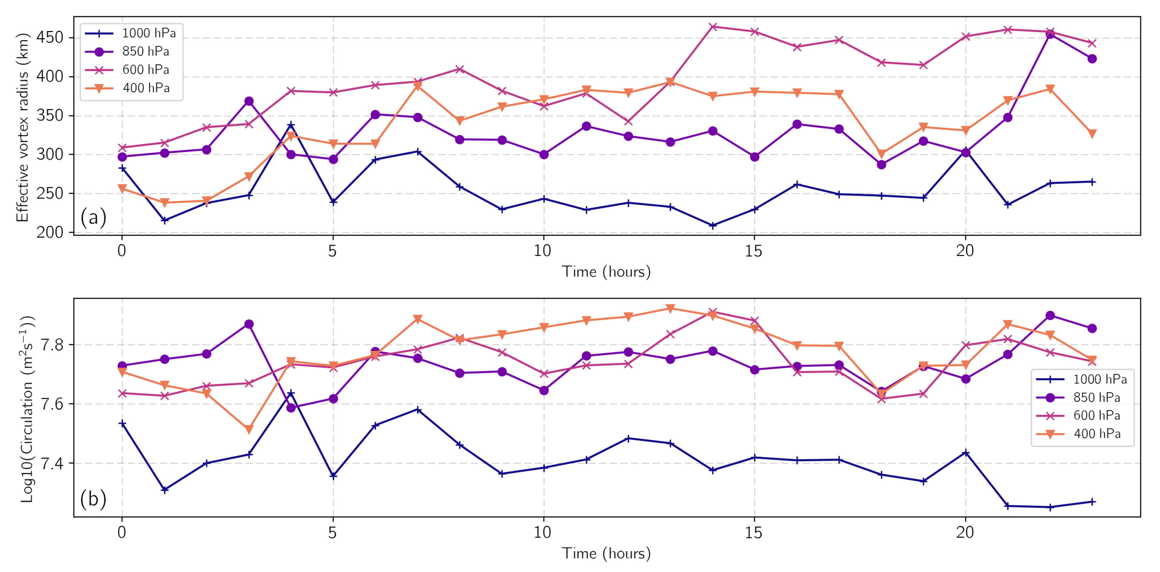
27]. In order to capture the vertical structure of Kyrill, we searched bottom-up for overlaps in the identified vortex patches fields starting at the lowest level. The locations of Kyrill derived from the NCEP data was used to identify the associated vortex structures in the other datasets. The best agreement between the different datasets was found for the 850-hPa level, while the upper levels showed a much stronger tilt for the NCEP data. This was probably due to the coarse resolution of the NCEP data and the generally larger vortices identified in NCEP. Hence, we used the location of NCEP-Kyrill at the 850-hPa level and its calculated effective radius as a mask for the upper and lower levels in CFSR and COSMO data. This means that only vortex systems that at least lied partially inside this mask were used to analyze the vertical structure of Kyrill in CFSR and COSMO data.
5. Discussion and Conclusions
In this work, we analyzed a high-impact extratropical cyclone with respect to its vortex properties in datasets of different horizontal grid spacing, covering the synoptic to the convective scales. The vortex properties were computed with the help of a single kinematic vortex identification method (-method). This method was based on the dimensionless kinematic vorticity number that differentiates between rotation-prevailing, i.e., vortices, vs. deformation-prevailing regions of the flow field. The main outcomes of this study were:
The -method was able to identify vortices throughout differently-resolved datasets in a reasonable manner, even at the convective scale.
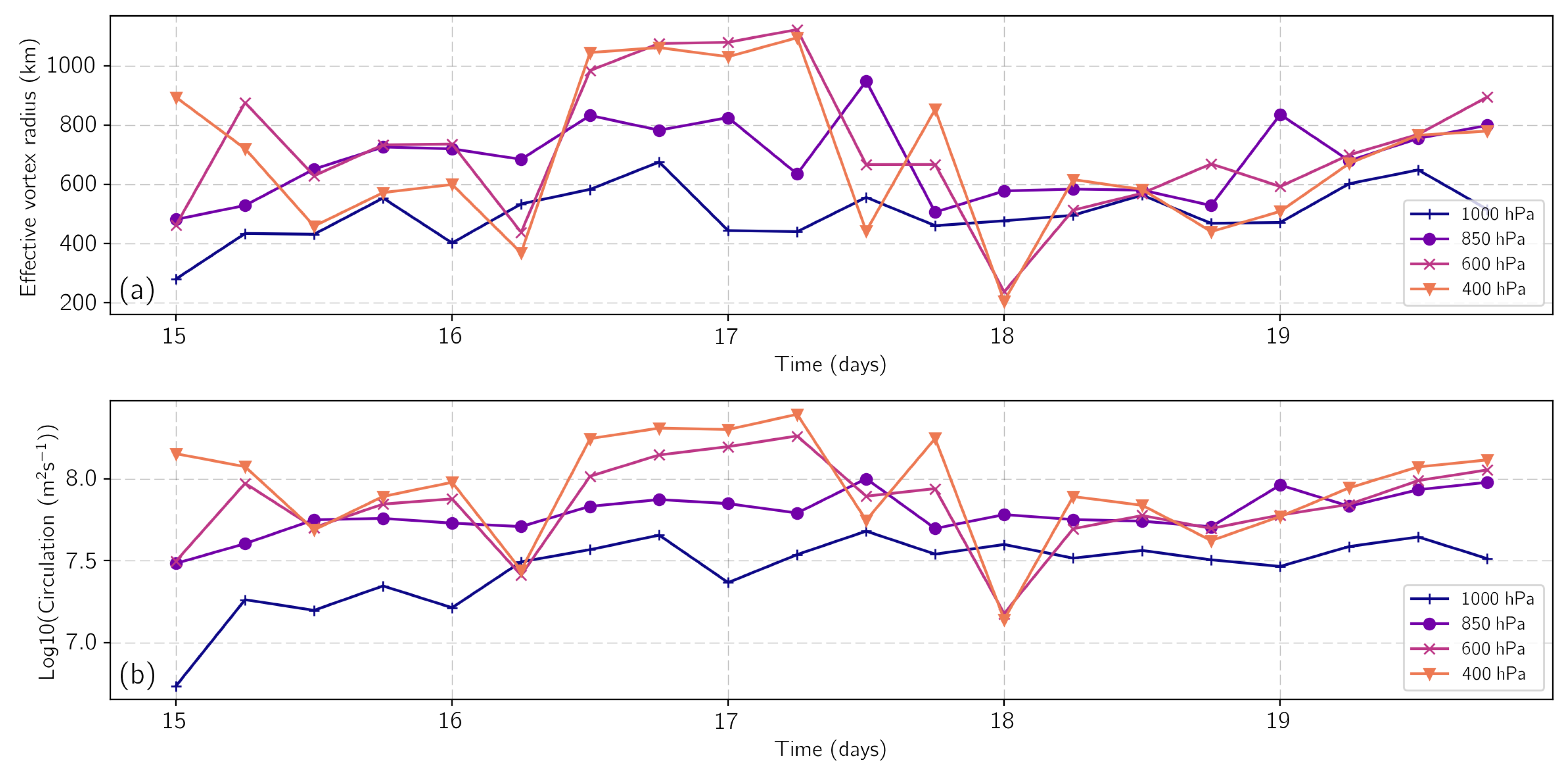
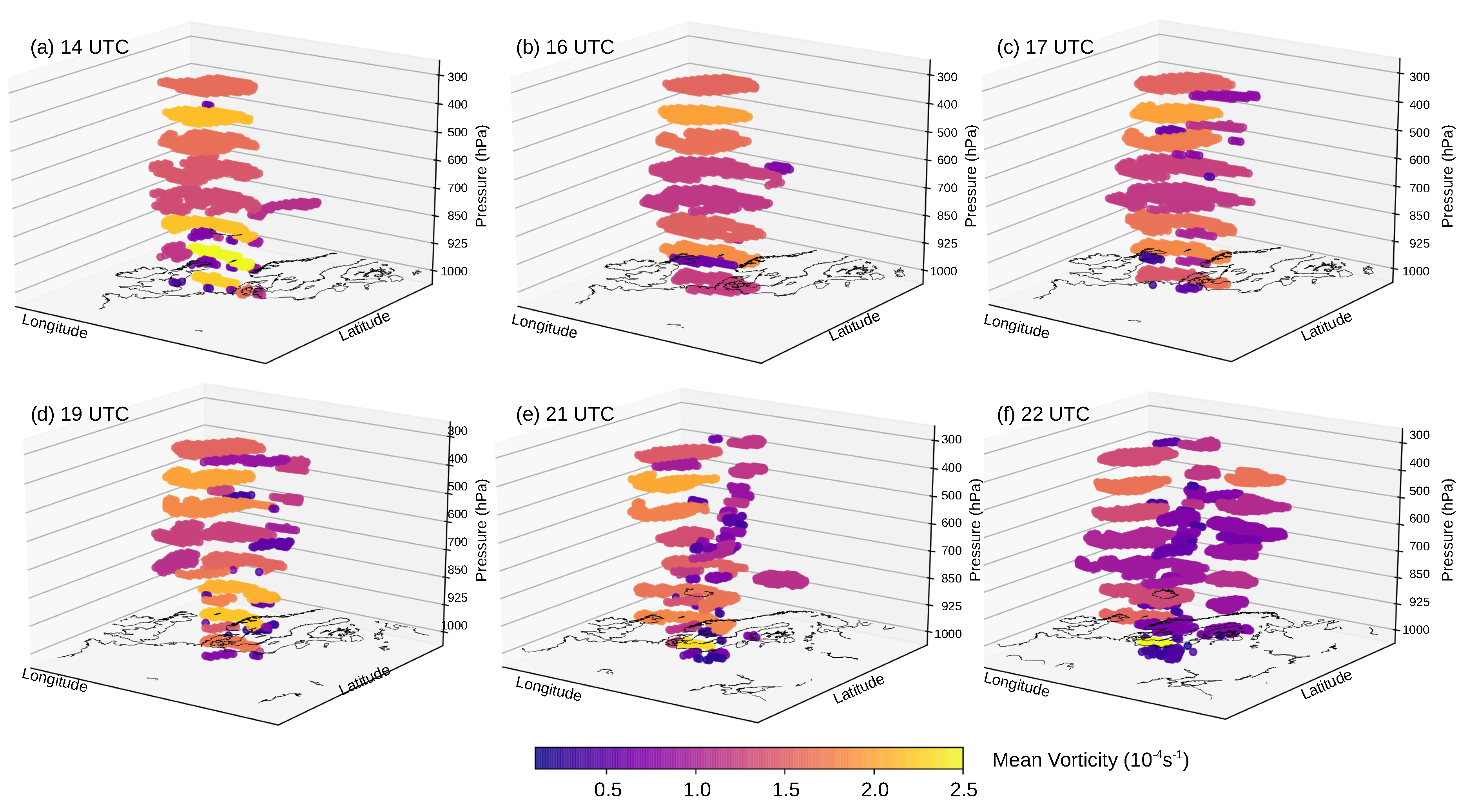
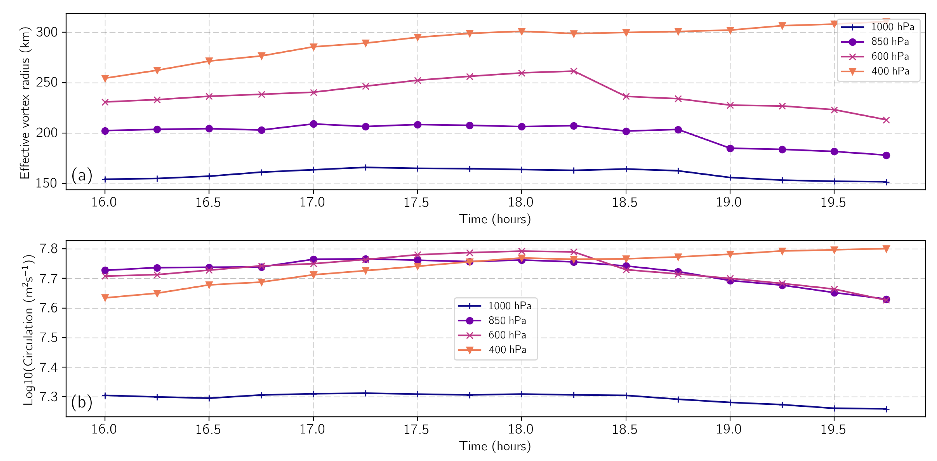
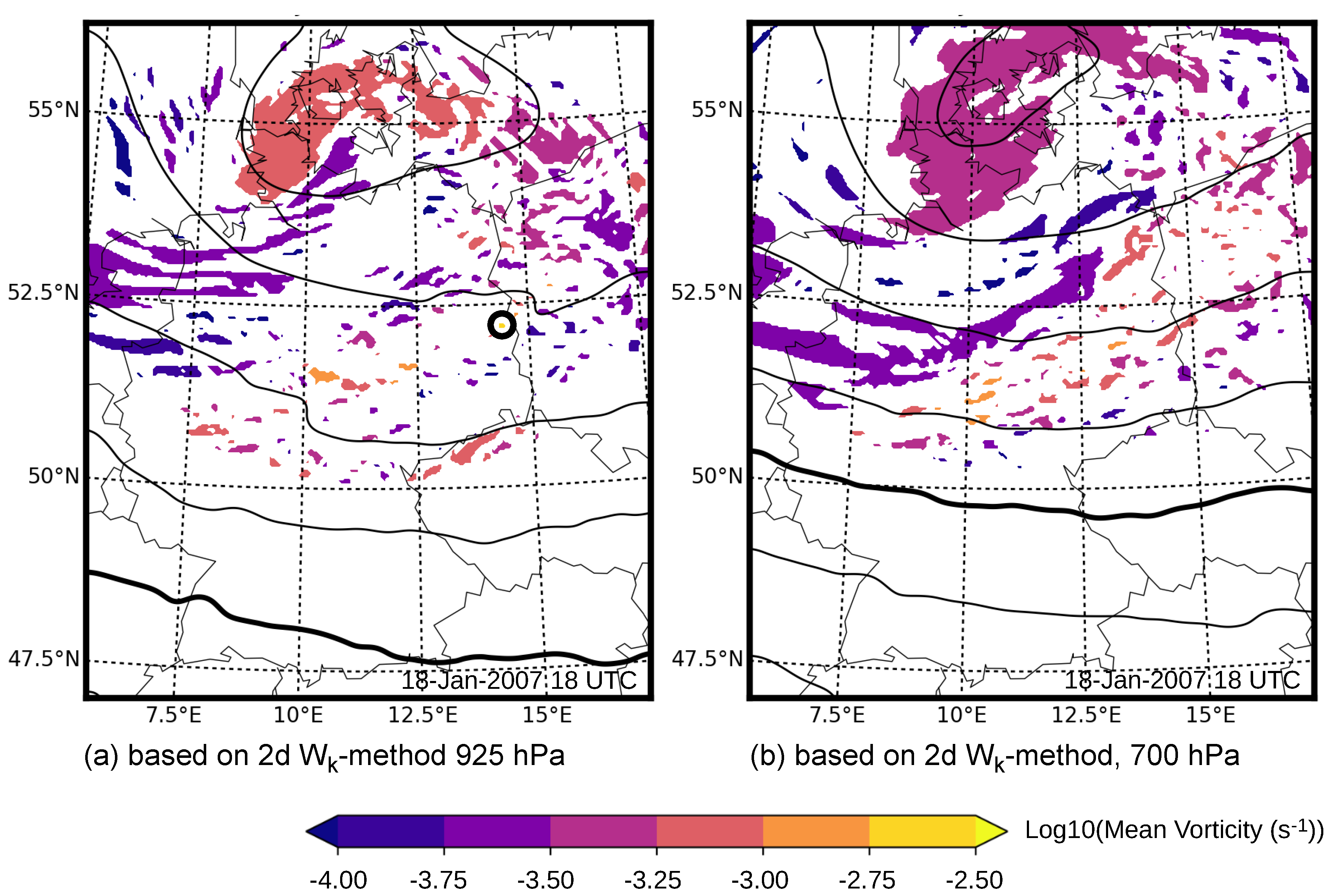
The identified vortices were in general larger in the upper troposphere and fragmented into smaller-scales in the lower troposphere.
The synoptic-scale storm system was composed of a large spectrum of vortex structures with varying horizontal scales and intensities.
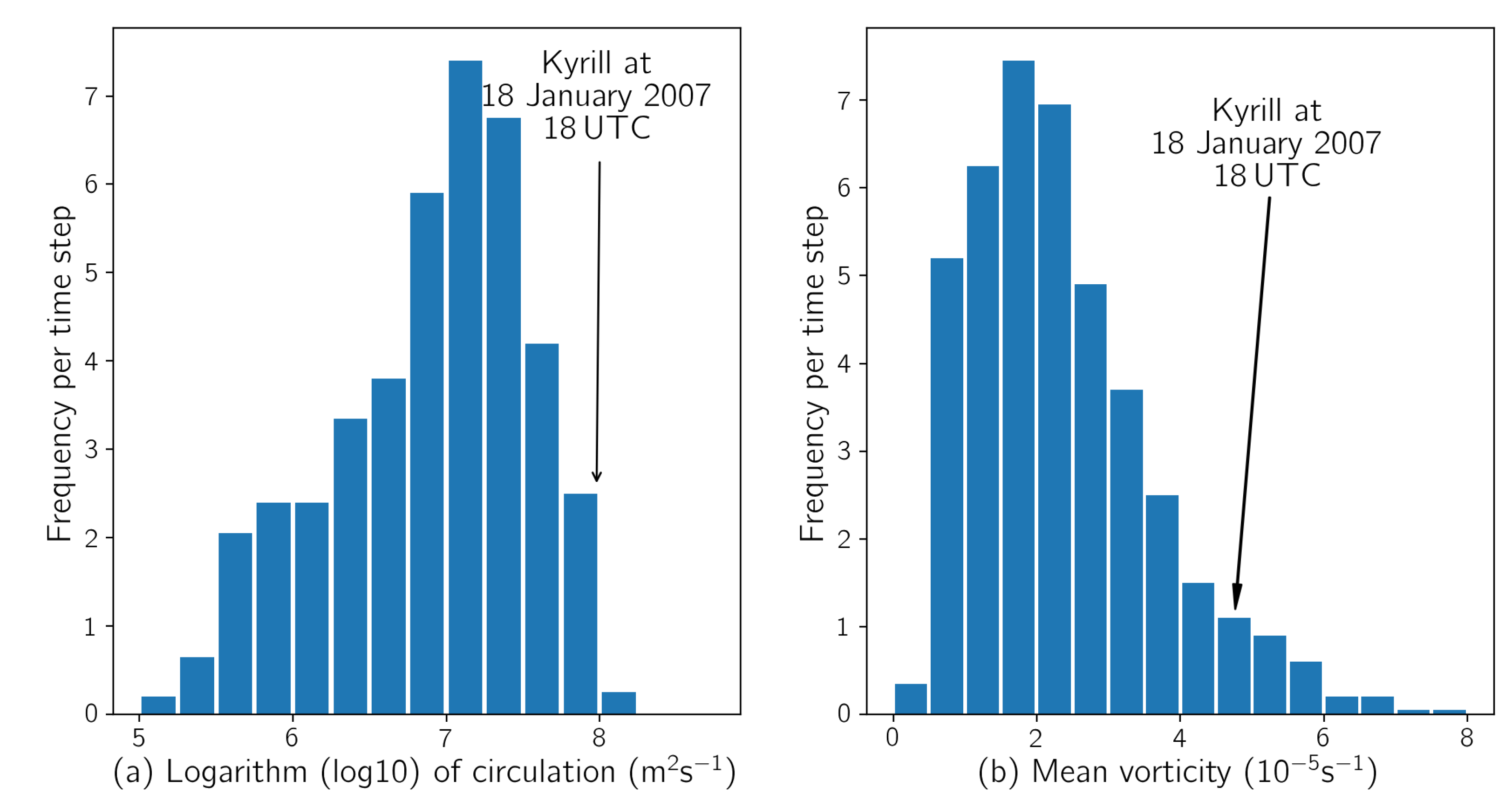
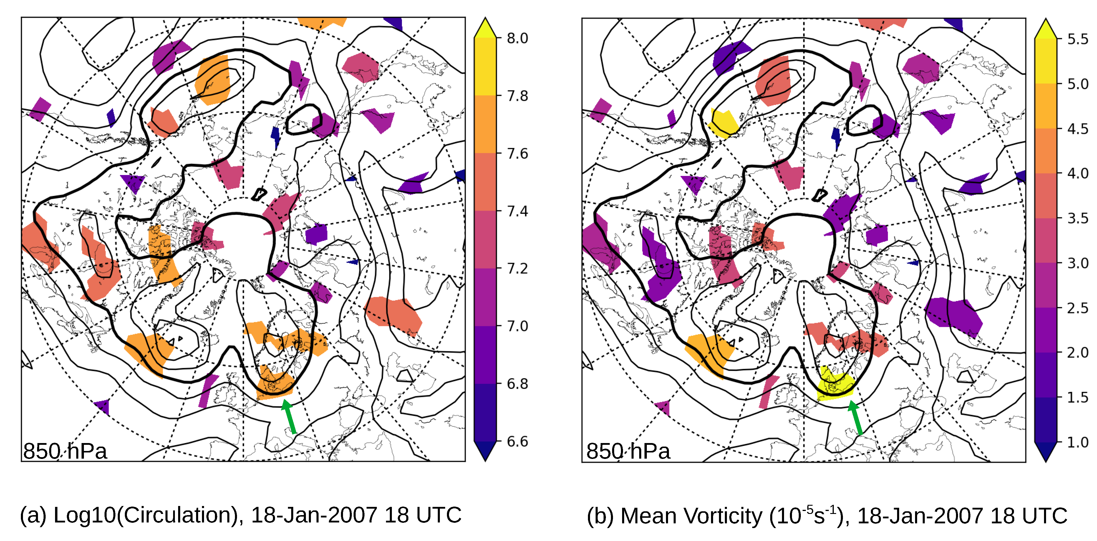
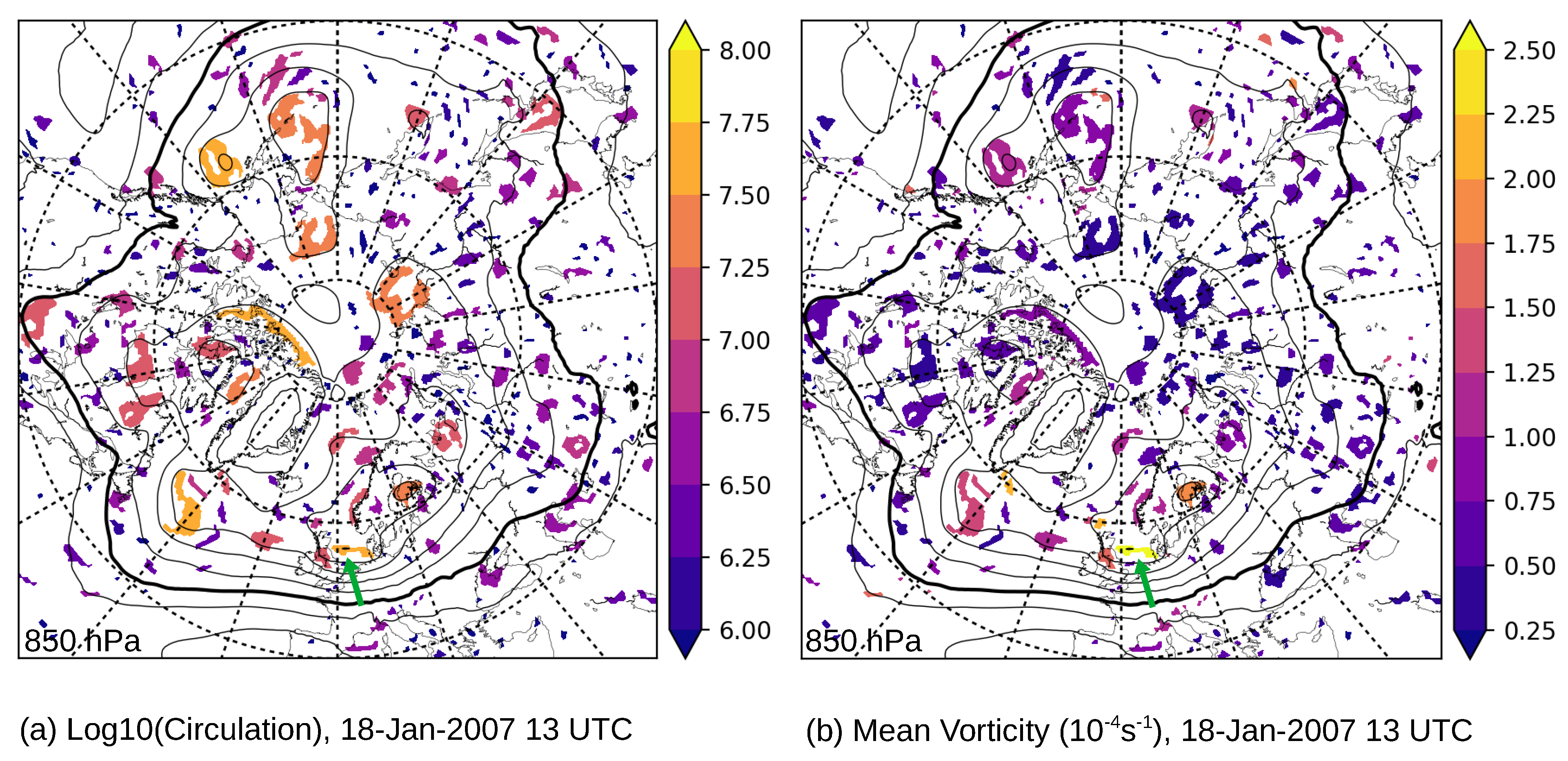
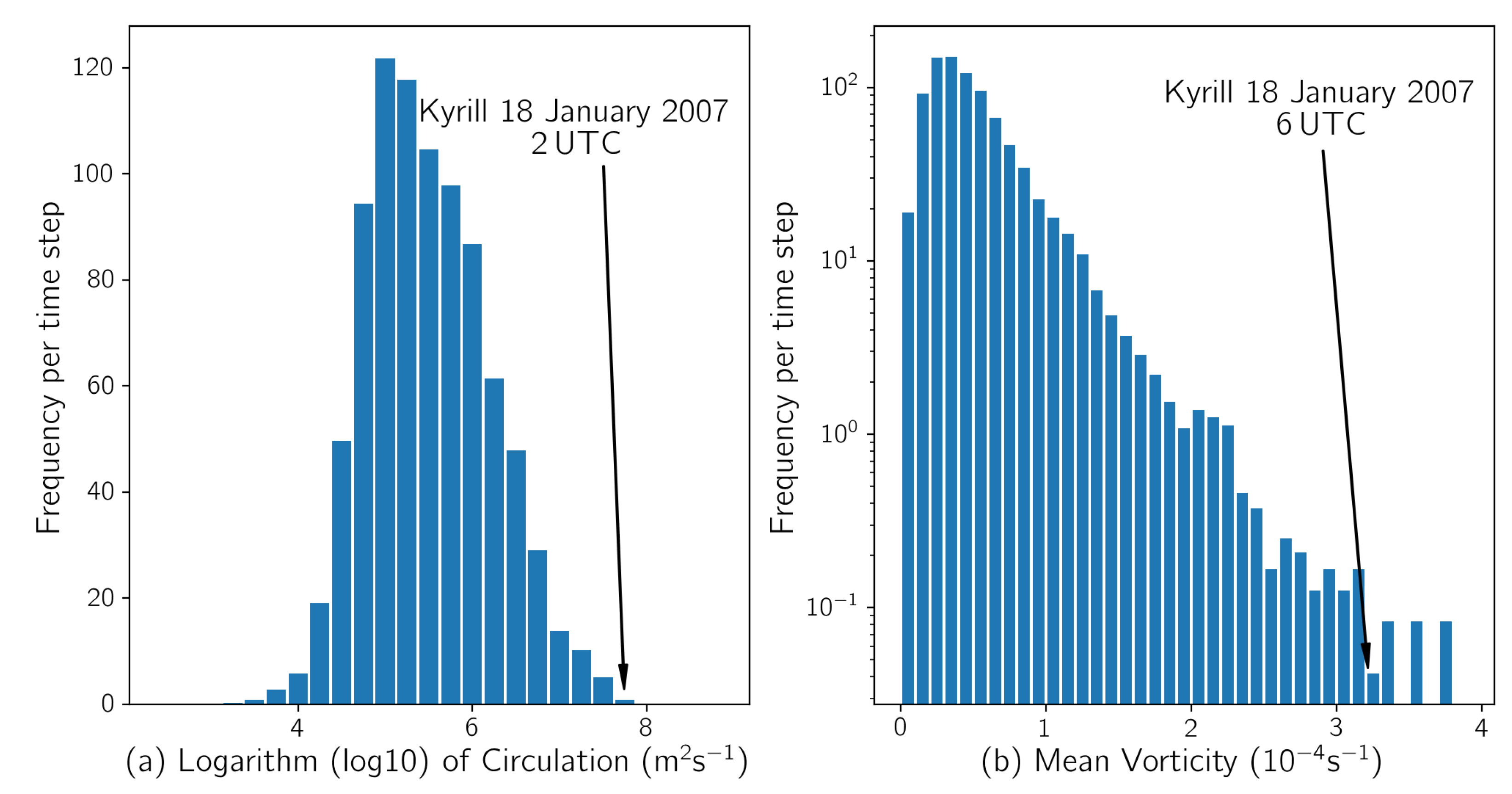
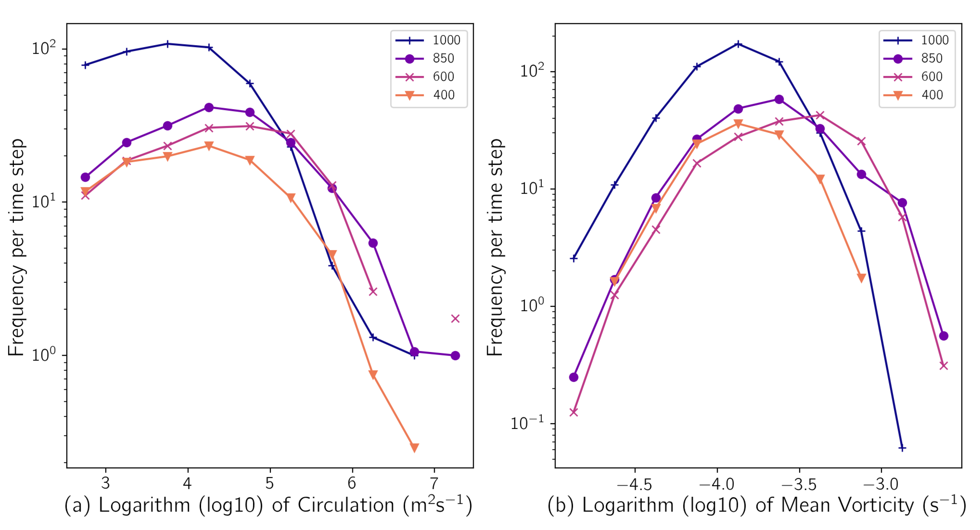
However, the total circulation of the system remained approximately constant across the scales, while the magnitude of the rather impact-related mean vorticity of the single vortices could increase considerably with increasing resolution.
The most surprising and, for us, impressive result was the almost complete conservation of the circulation throughout the different datasets. This has some implications with respect to the interpretation of vortex intensities in climate change studies: if an increase in the synoptic-scale circulations were observed in future scenarios, the intensity of smaller-scale embedded vortices could increase, as well. Though it was not clear which intensity measure was the best and this problem possibly depends significantly on the research question, we were positively surprised by the performance of circulation and mean vorticity. Color shading the vortices by their mean vorticity on the other hand seemed to highlight the intense, impact-related vortices such as the ones that occurred along Kyrill’s cold front. Though the plots needed scale-dependent adjustments considering the vorticity range, they could still be a useful tool, especially with respect to the forecast of high-impact weather. However, besides single case studies, a detailed climatological analysis should be done in future work to further explore the benefits of the -method.
We already knew that the vorticity was a scale-dependent variable, e.g., [
12], and that vorticity-related measures such as the potential vorticity were scale-dependent, as in [
41], who studied the sensitivity of resolution on a tropical cyclone with horizontal grid spacings between 1 and 8 km. With our study, we can confirm that the vorticity magnitudes indeed increased with increasing resolutions. Additionally, we can explicitly calculate the distribution of mean vorticity and circulation magnitudes. The sizes of the resolved vortices showed a large spectrum of effective radii, in particular in the higher-resolved datasets. Even in the high-resolution COSMO data, we still observed a (sub-)synoptic-scale vortex that represented the central core of Kyrill and a multitude of vortices with different scales that were associated with fronts and convective cells. We summarize these important results in
Table 1.
Our observation that the size of extratropical cyclones in general increased with height was also found in Lim and Simmonds [
42], who based their vortex identification on the Laplacian of the pressure (the Laplacian of pressure is proportional to the geostrophic vorticity). We can now further confirm that this general increase also occurred in data with higher resolution. However, Lim and Simmonds [
42] did not describe a possible fragmentation of an upper-level vortex into smaller-scale vortices in the lower troposphere. Those structures were perhaps missing due to the removal of less intense systems in advance. The fragmentation was also documented in some example cases given in [
43], who used a 4D tracking algorithm to study the four-dimensional structure of Southern Hemisphere low-pressure systems based on the anomaly fields of the vertical vorticity. Understanding the reasons for this fragmentation and its connection to viscous processes could be an interesting topic for future studies, especially since the contraction of the vortex area led to an intensification due to the (quasi-)conservation of the circulation.
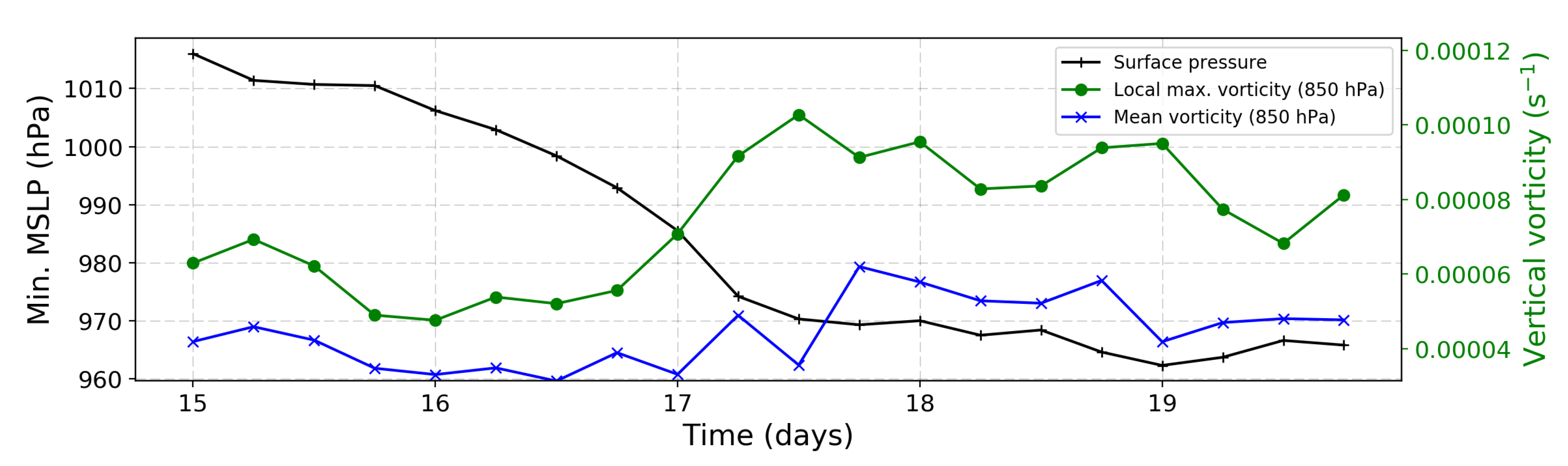
Finally, we were able to display some characteristics of the high-impact event addressed in the literature. The
-method can identify the processes of explosive intensification of Kyrill and secondary cyclogenesis in accordance with the publications of [
27,
29]. With the additional knowledge of the vortex size and the use of different intensity measures, the visualization of these processes was quite clear, especially the secondary cyclogenesis and even in the coarsely-resolved NCEP data.
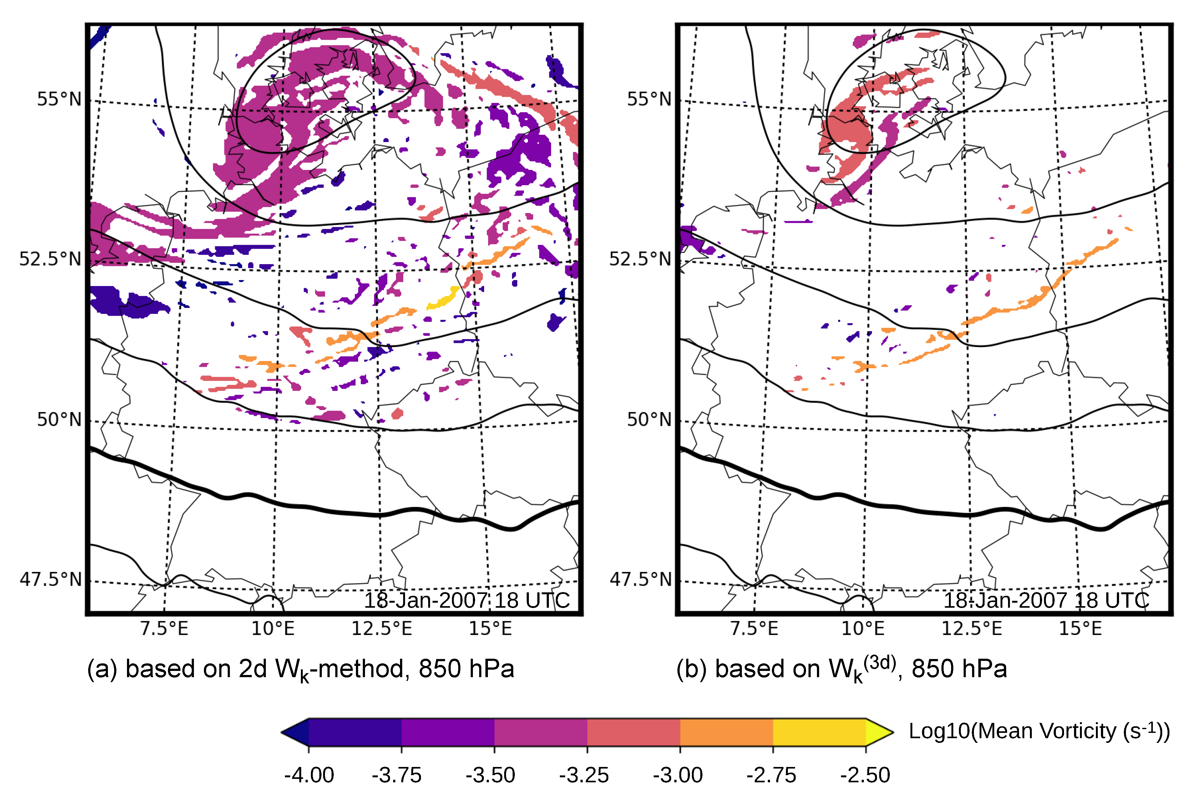
At high resolution, our method highlighted deep moist convection, including information on the convective storm mode such as bowing segments and bookend vortices and regions of high winds. A surprising result was the different identification of vortex structures for the two-dimensional and the three-dimension
-method. Although the
-method identified the stronger vortices with higher mean vorticities in the lower levels similar to the 2D
-method, it is important to understand what the unidentified vortices were. These were likely related to convective cells or waves with upward and downward motions that appeared as a vortex in the 2D
fields. The two-dimensional kinematic vorticity number assumed that the vortex rotated around an approximately vertical axis and only compared the vertical vorticity with the deformational flow components at the horizontal level. Kyrill was a storm system that interacted with the upper-level jet stream [
29]. Hence, the environment of the convection was characterized by strong vertical wind shear. This also implied large horizontal vorticity components. Due to up- and down-drafts, these vorticity lines were tilted up- or downwards, generating vertical vorticity. The magnitude of the vertical vorticity was in large parts of the field higher than the strain-rate, and hence, a vortex was identified. A change to the three-dimensional
-method revealed that the associated three-dimensional strain-rates were higher or at least of comparable order to the vorticity vector components.
In summary, the -method performed well in the data of different resolutions and at different height levels. The proposed color shading by intensity measures seemed to highlight potentially high-impact vortices. The method might be of interest to a variety of topics, including teaching, mesoscale meteorology, storm dynamics, climate research, and storm risk estimation. Therefore, the -method is a promising tool for various future applications.


