Analysis of a Case of Supercellular Convection over Bulgaria: Observations and Numerical Simulations

Abstract
1. Introduction
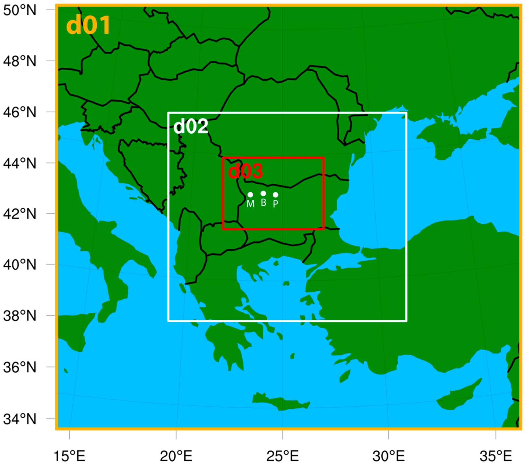
2. Data and Methods
2.1. Observations
2.2. Numerical Weather Prediction Data
3. Results
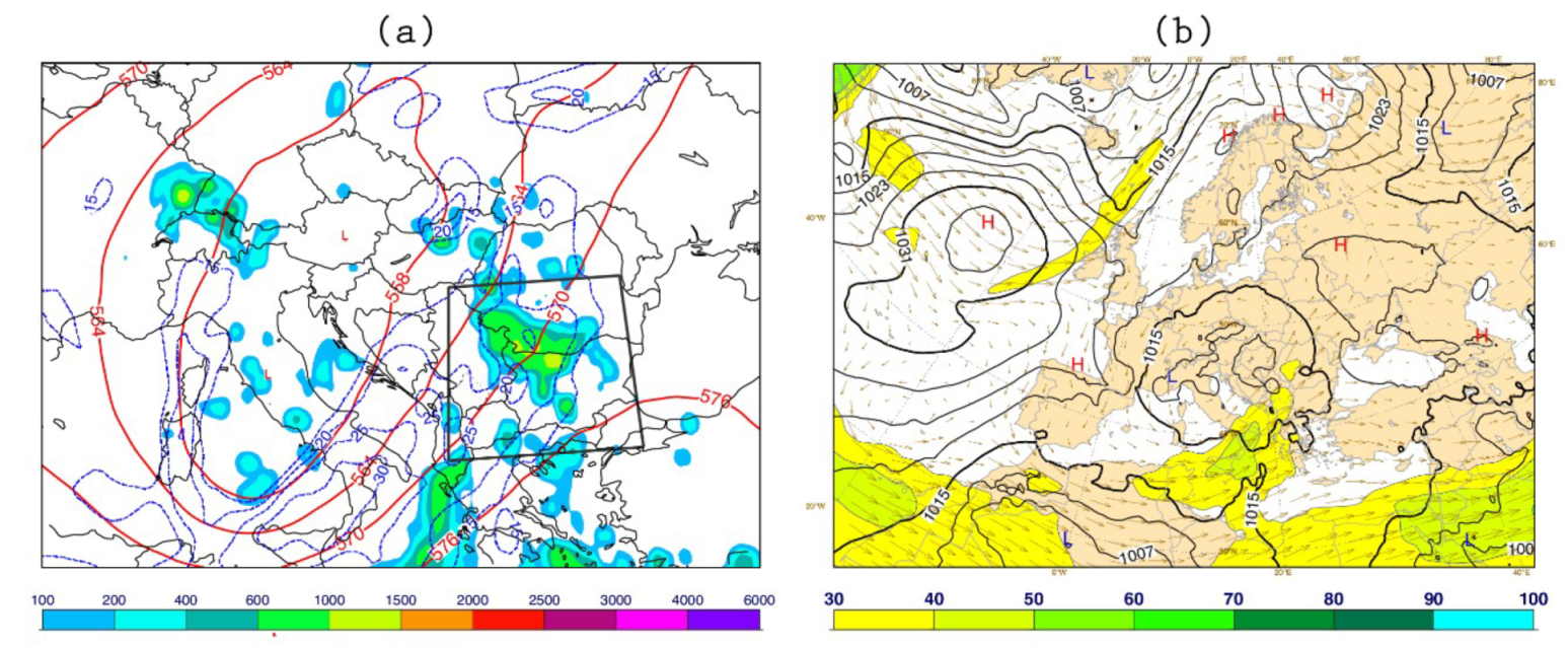
3.1. Description of the Event
3.2. Observed Evolution of the Supercell
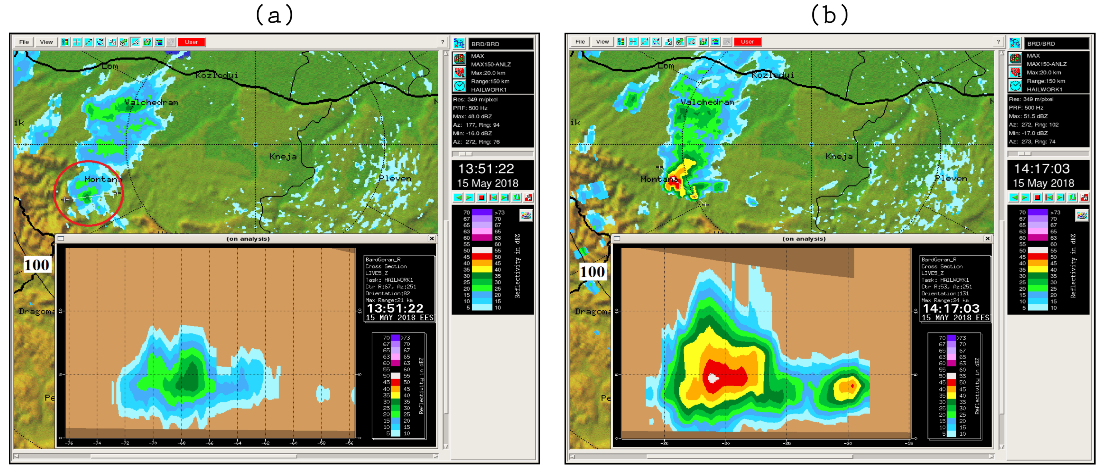
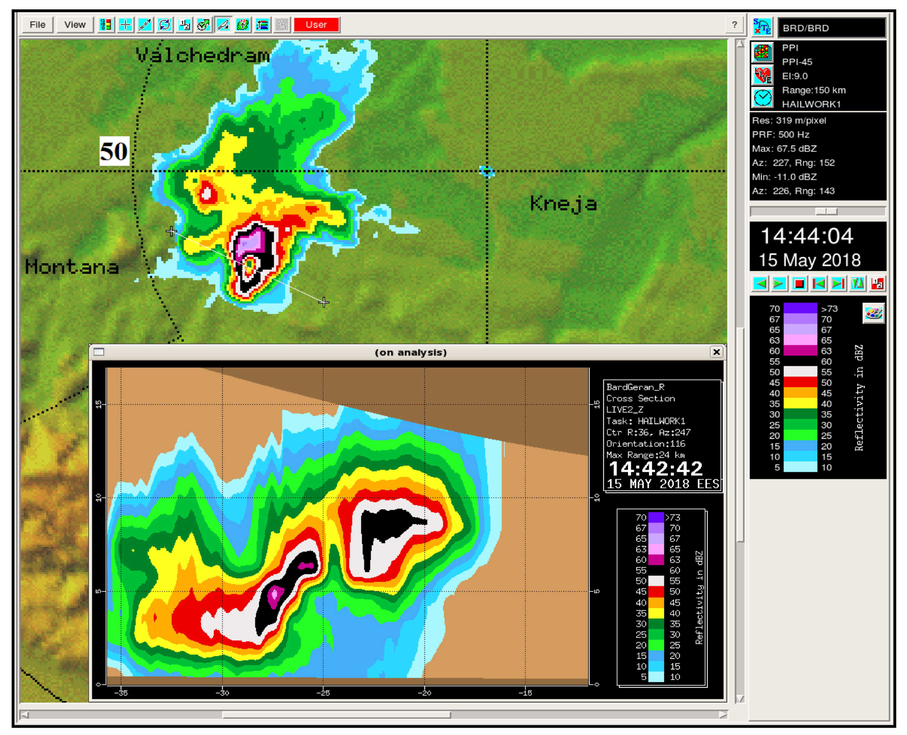
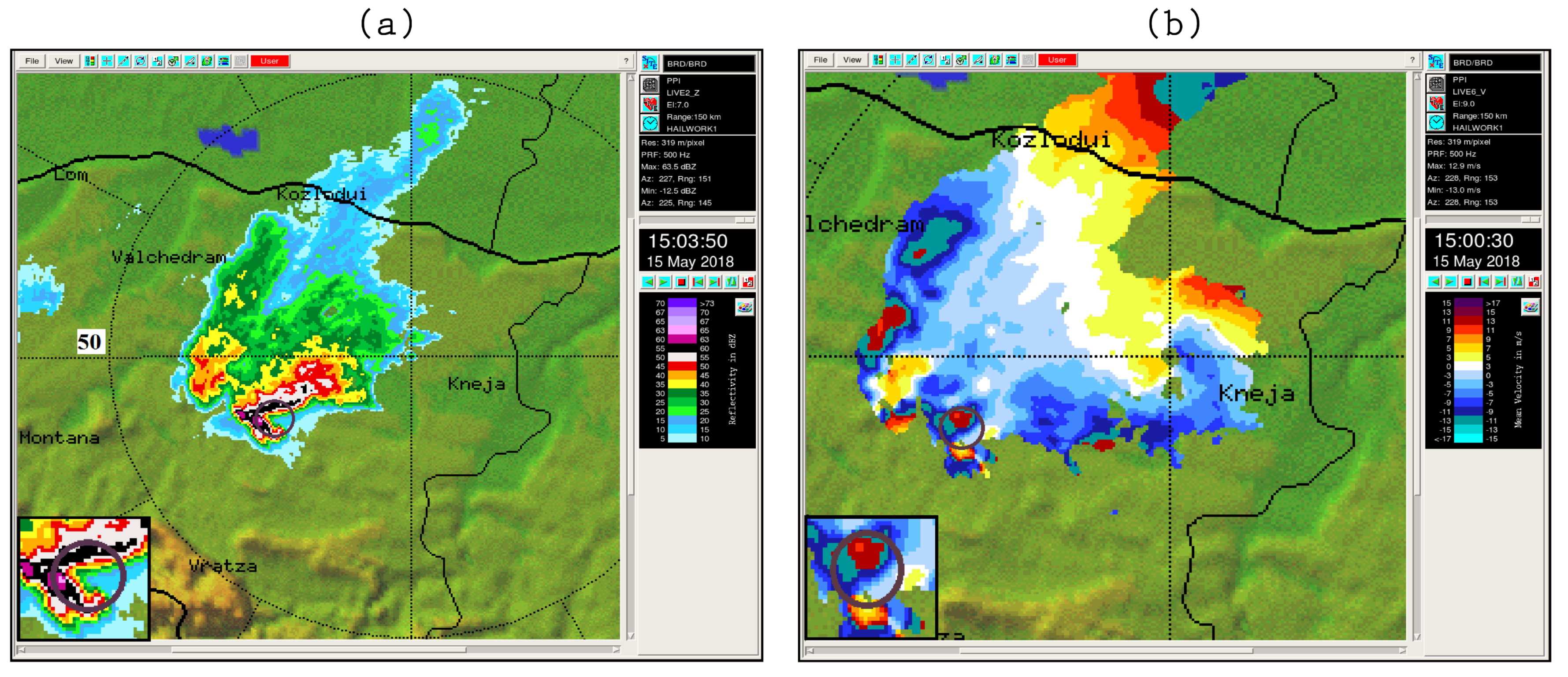
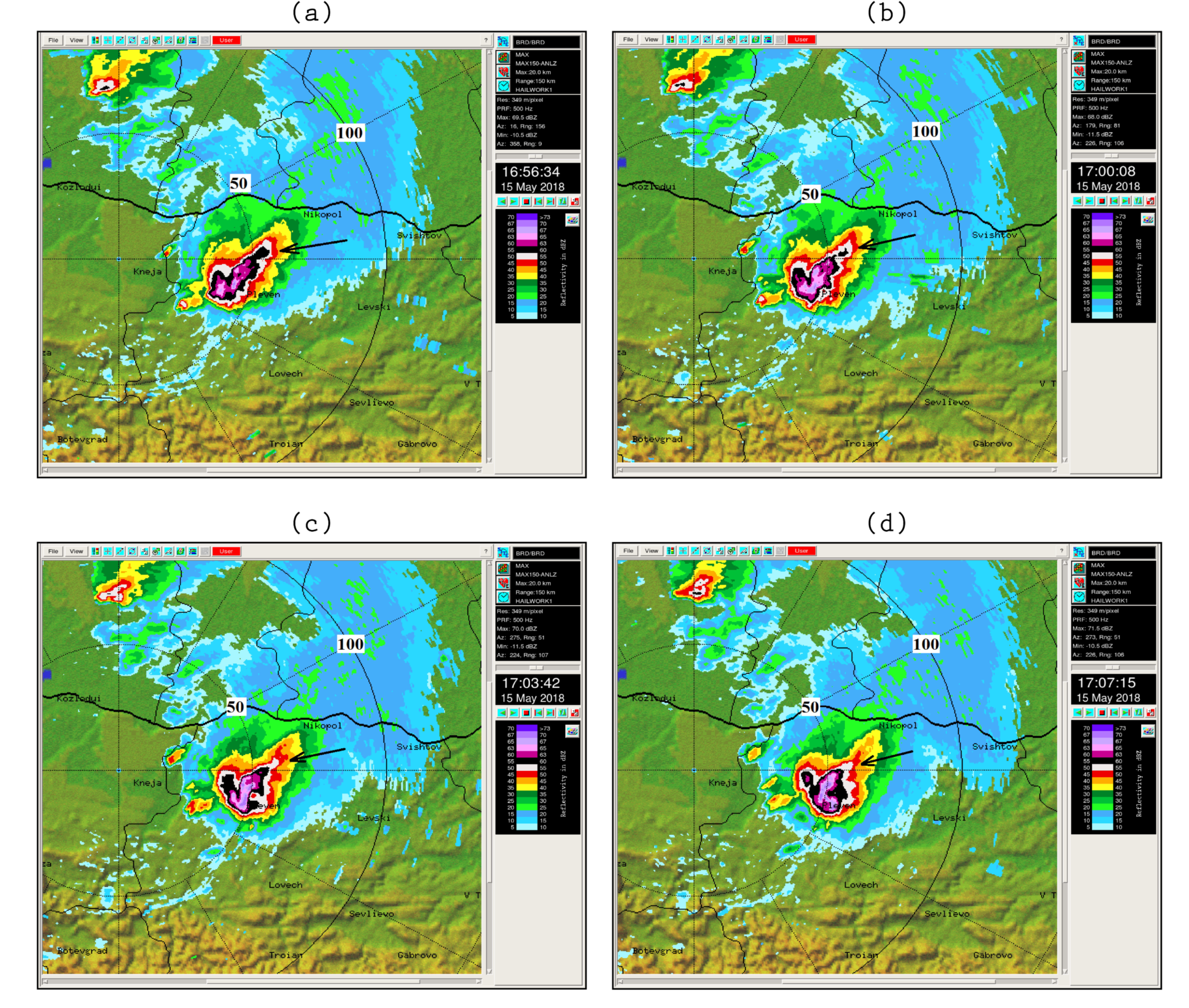
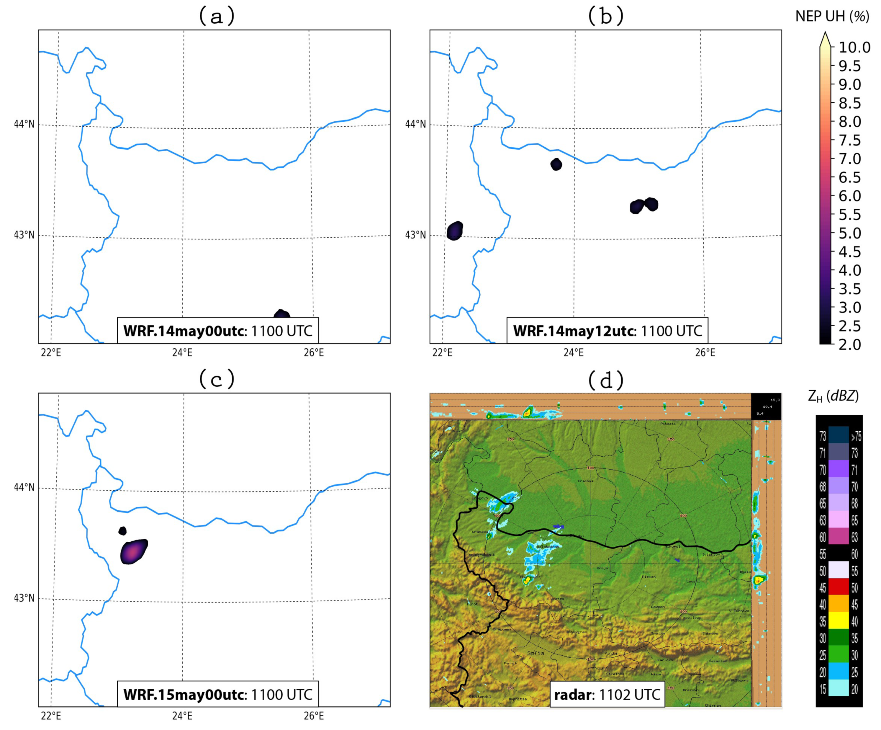
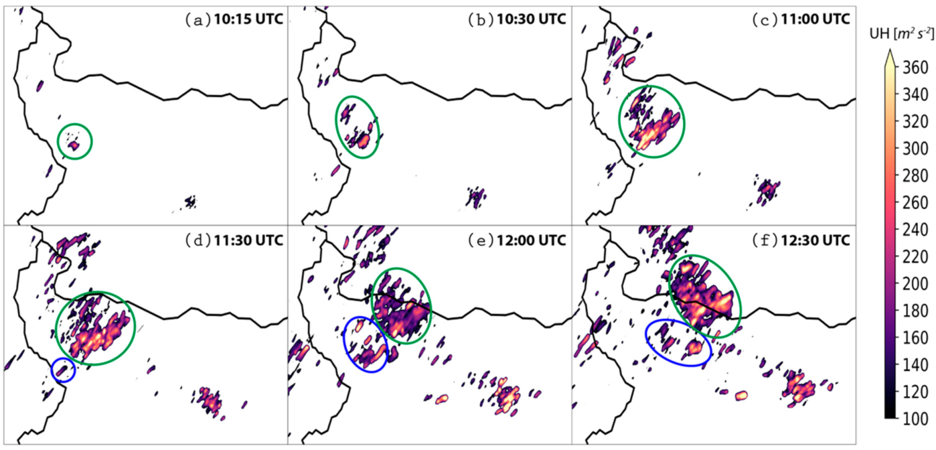
3.2.1. Radar Analysis
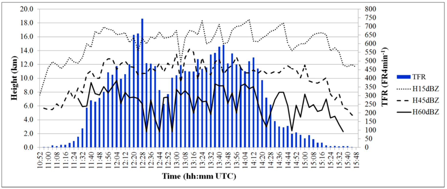
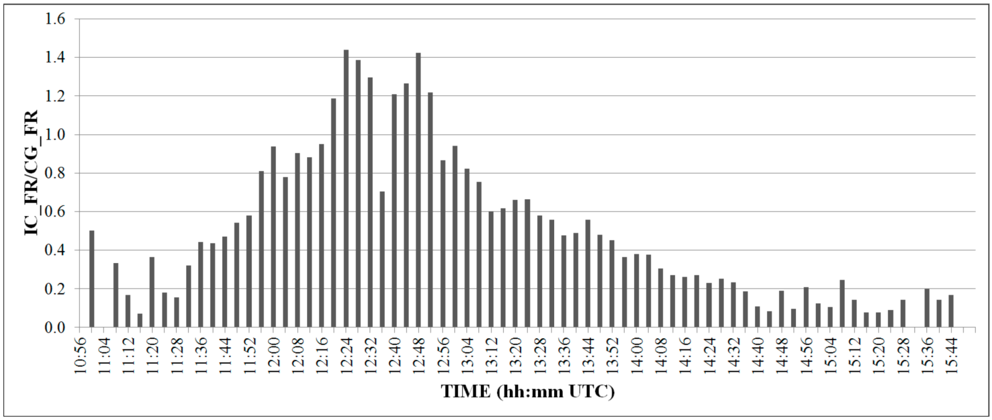
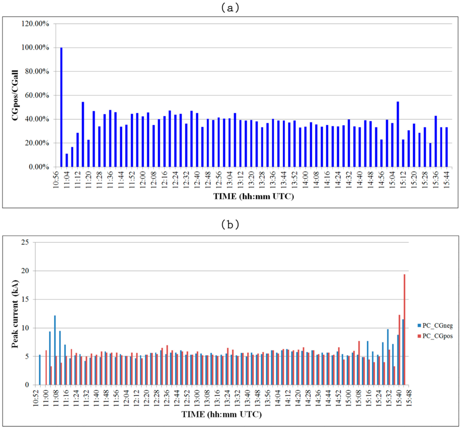
3.2.2. Lightning Activity
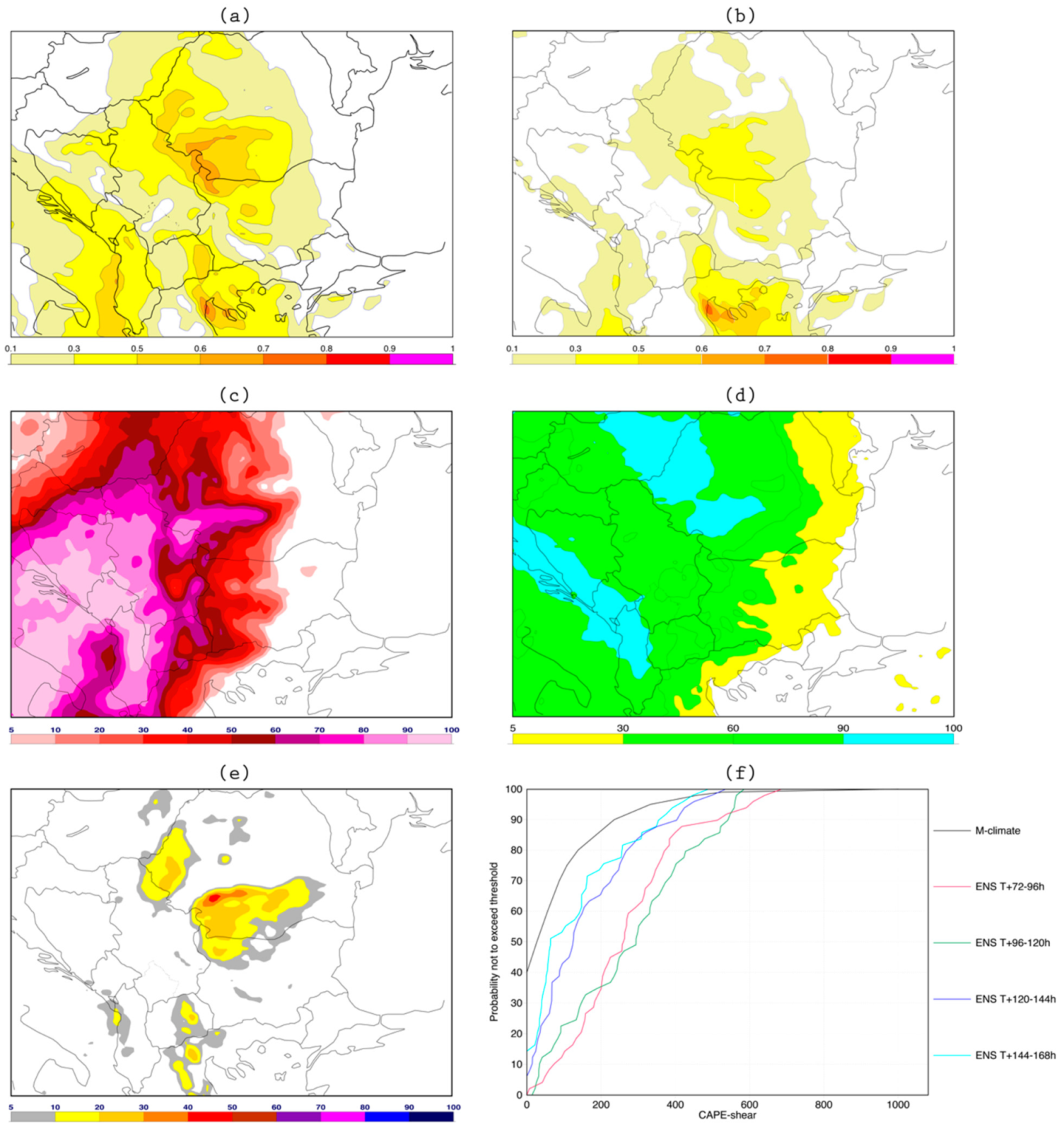
3.3. Forecasts from the Global ECMWF Ensemble
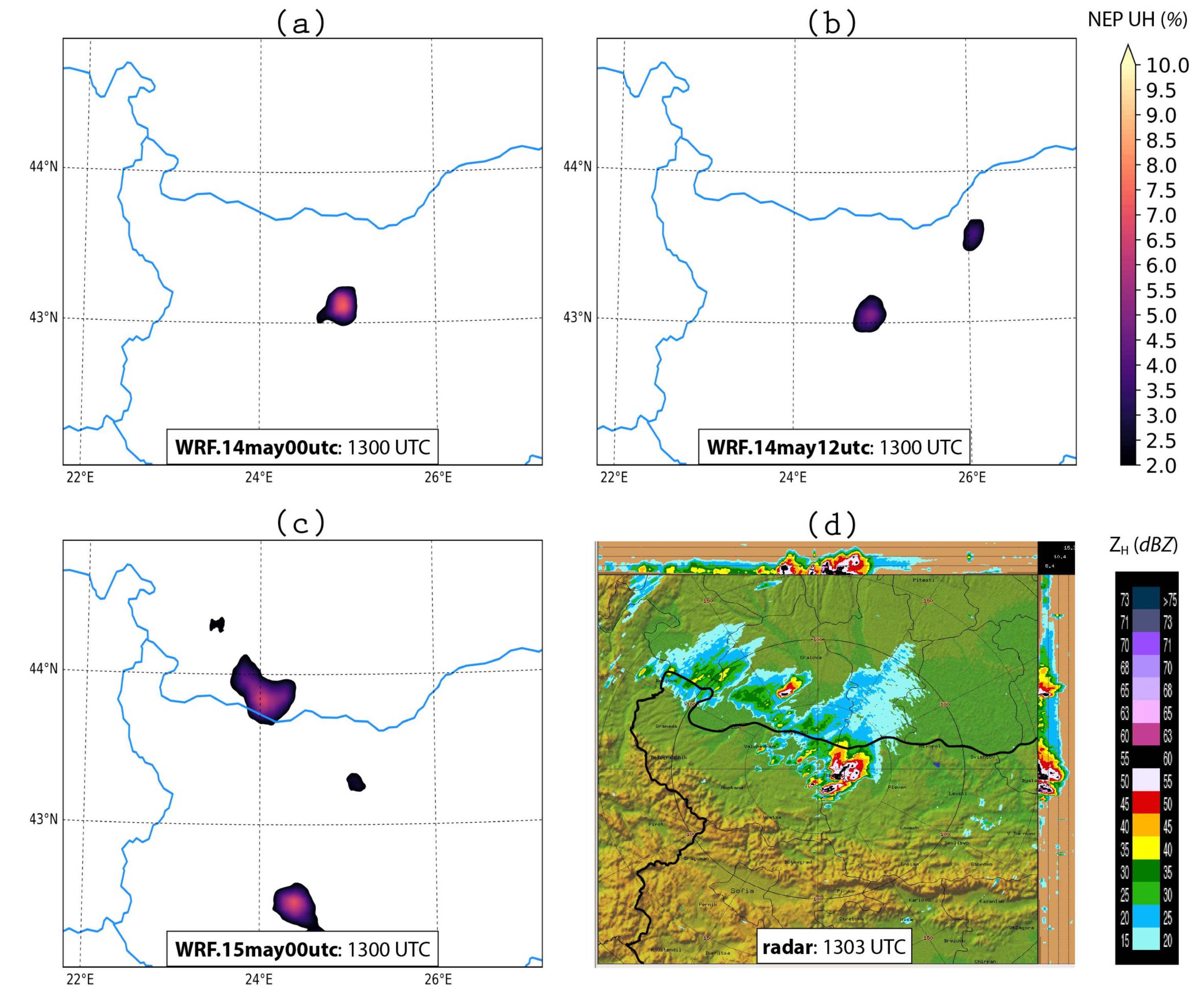
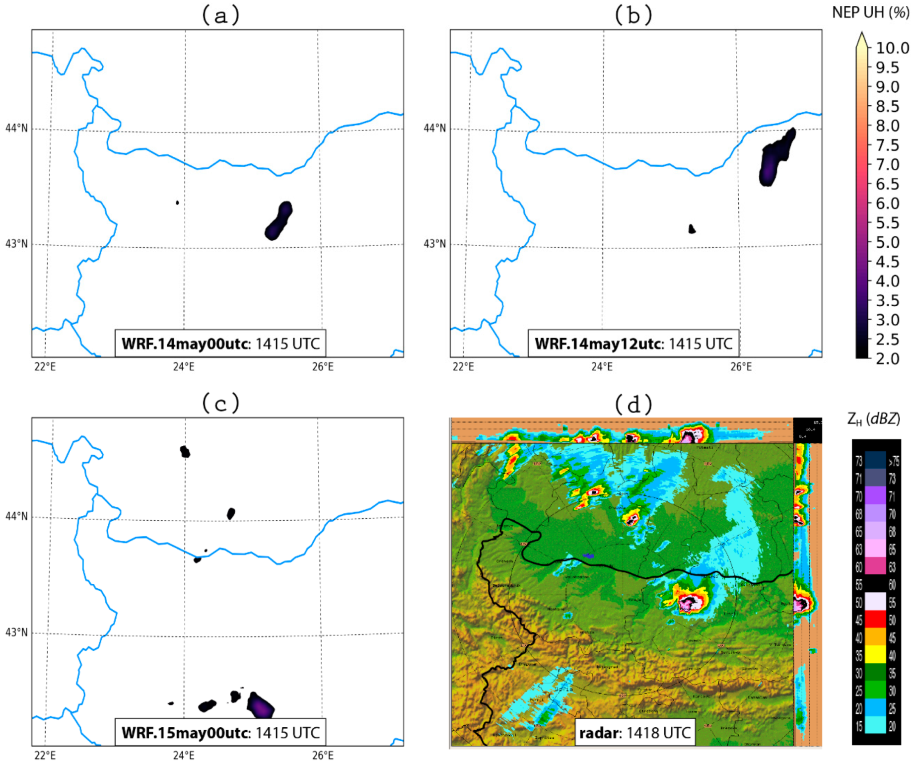
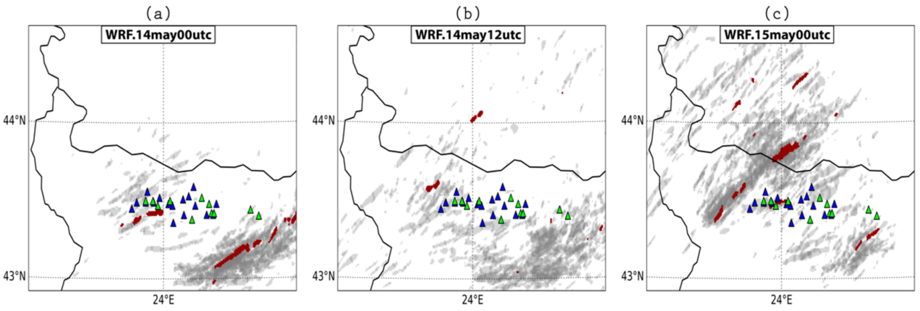
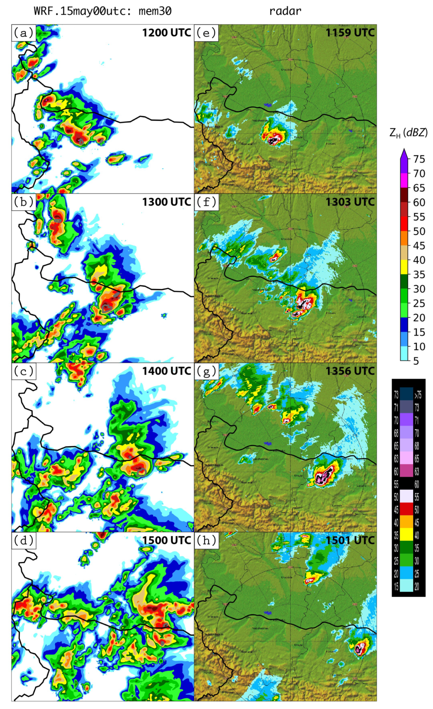
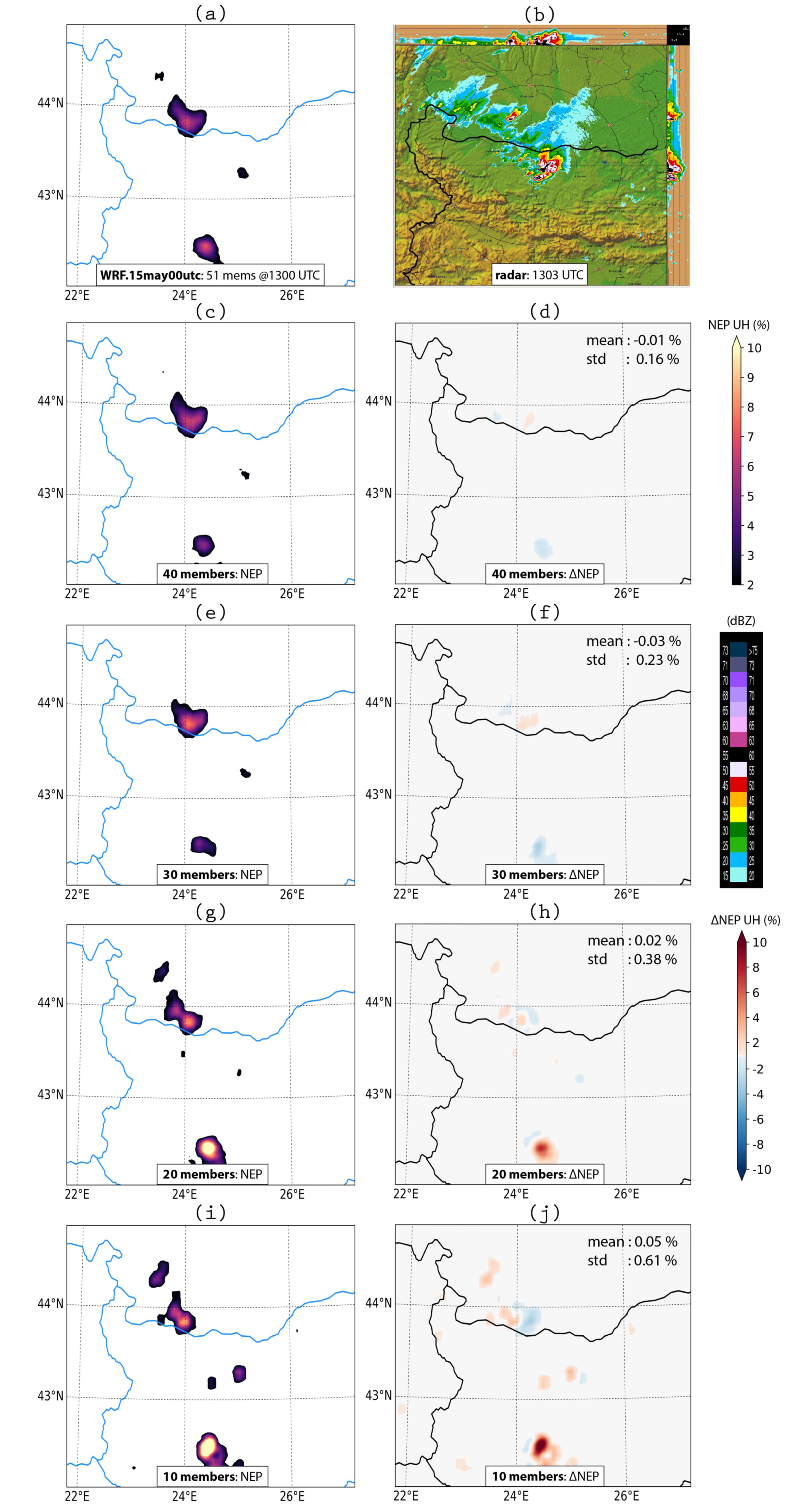
3.4. Explicit Convective Forecasts from the WRF Ensemble
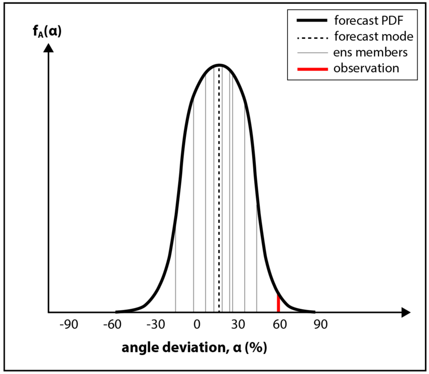
3.4.1. Predictability
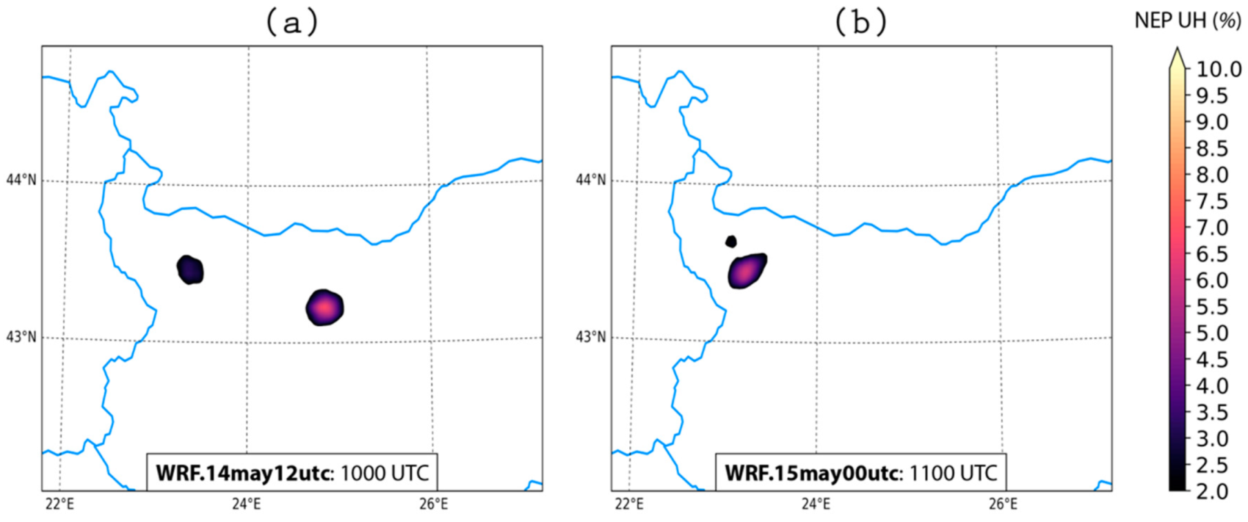
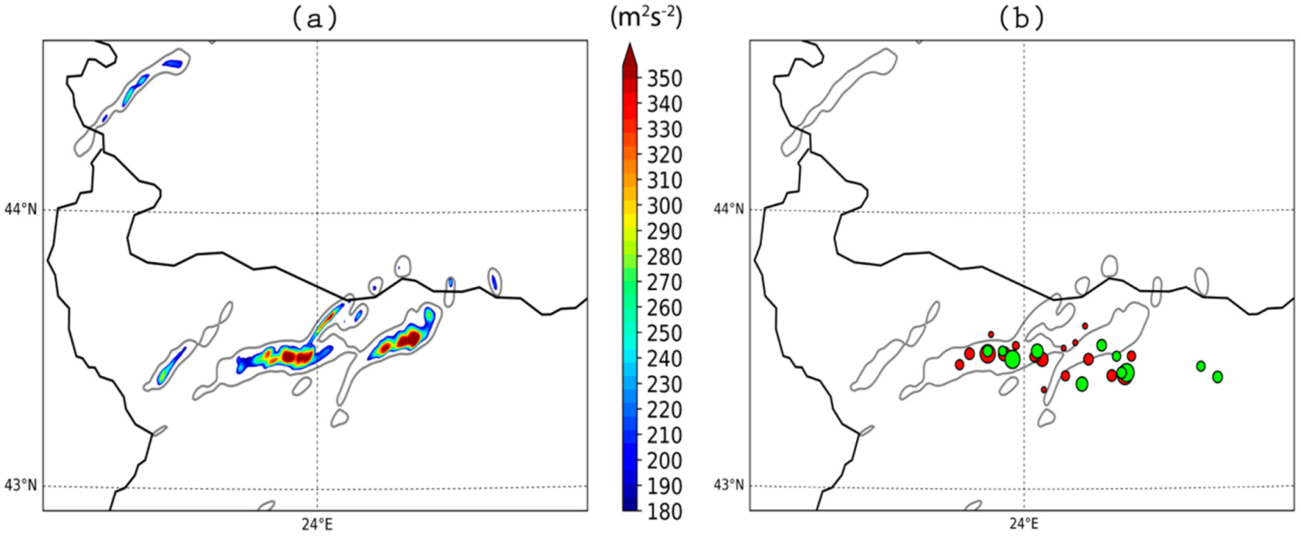
3.4.2. Ensemble Clustering
3.4.3. Model Errors in CAM-Based Ensembles
4. Conclusions
- the timing of convection initiation (CI);
- the large amounts of spurious convection in proximity to the simulated supercell.
5. Outlook
Author Contributions
Funding
Acknowledgments
Conflicts of Interest
References
- Groenemeijer, P.; Kühne, T.; Groenemeijer, P.; Kühne, T. A Climatology of Tornadoes in Europe: Results from the European Severe Weather Database. Mon. Wea. Rev. 2014, 142, 4775–4790. [Google Scholar] [CrossRef]
- Antonescu, B.; Schultz, D.M.; Holzer, A.; Groenemeijer, P.; Antonescu, B.; Schultz, D.M.; Holzer, A.; Groenemeijer, P. Tornadoes in Europe: An Underestimated Threat. Bull. Am. Meteorol. Soc. 2017, 98, 713–728. [Google Scholar] [CrossRef]
- Antonescu, B.; Cărbunaru, F.; Antonescu, B.; Cărbunaru, F. Lightning-Related Fatalities in Romania from 1999 to 2015. Weather. Clim. Soc. 2018, 10, 241–252. [Google Scholar] [CrossRef]
- Dotzek, N.; Groenemeijer, P.; Feuerstein, B.; Holzer, A.M. Overview of ESSL’s severe convective storms research using the European Severe Weather Database ESWD. Atmos. Res. 2009, 93, 575–586. [Google Scholar] [CrossRef]
- Taszarek, M.; Allen, J.; Púčik, T.; Groenemeijer, P.; Czernecki, B.; Kolendowicz, L.; Lagouvardos, K.; Kotroni, V.; Schulz, W.; Taszarek, M.; et al. A Climatology of Thunderstorms across Europe from a Synthesis of Multiple Data Sources. J. Clim. 2019, 32, 1813–1837. [Google Scholar] [CrossRef]
- Púčik, T.; Groenemeijer, P.; Rýva, D.; Kolář, M.; Púčik, T.; Groenemeijer, P.; Rýva, D.; Kolář, M. Proximity Soundings of Severe and Nonsevere Thunderstorms in Central Europe. Mon. Wea. Rev. 2015, 143, 4805–4821. [Google Scholar] [CrossRef]
- Browning, K.A. The Structure and Mechanisms of Hailstorms. In Hail: A Review of Hail Science and Hail Suppression; American Meteorological Society: Boston, MA, 1977; pp. 1–47. [Google Scholar]
- Weisman, M.L.; Klemp, J.B. The Dependence of Numerically Simulated Convective Storms on Vertical Wind Shear and Buoyancy. Mon. Wea. Rev. 1982, 110, 504–520. [Google Scholar] [CrossRef]
- Weisman, M.L.; Klemp, J.B.; Weisman, M.L.; Klemp, J.B. The Structure and Classification of Numerically Simulated Convective Stormsin Directionally Varying Wind Shears. Mon. Wea. Rev. 1984, 112, 2479–2498. [Google Scholar] [CrossRef]
- Davies-Jones, R. A review of supercell and tornado dynamics. In Atmospheric Research; Elsevier: Amsterdam, The Netherlands, 2015; Volume 158–159, pp. 274–291. [Google Scholar]
- Rotunno, R.; Klemp, J.B.; Rotunno, R.; Klemp, J.B. The Influence of the Shear-Induced Pressure Gradient on Thunderstorm Motion. Mon. Wea. Rev. 1982, 110, 136–151. [Google Scholar] [CrossRef]
- Brooks, H.E.; Doswell, C.A.; Cooper, J.; Brooks, H.E.; III, C.A.D.; Cooper, J. On the Environments of Tornadic and Nontornadic Mesocyclones. Wea. Forecasting 1994, 9, 606–618. [Google Scholar] [CrossRef]
- Lemon, L.R.; Doswell, C.A.; Lemon, L.R.; III, C.A.D. Severe Thunderstorm Evolution and Mesocyclone Structure as Related to Tornadogenesis. Mon. Wea. Rev. 1979, 107, 1184–1197. [Google Scholar] [CrossRef]
- Doswell, C.A.; Burgess, D.W. Tornadoes and toraadic storms: A review of conceptual models. Geophys. Monogr.-Am. Geophys. Union 1993, 79, 161–172. [Google Scholar]
- Maier, M.W.; Krider, E.P. A comparative study of cloud-to-ground lightning characteristics in Florida and Oklahoma thunderstorms. In Proceedings of the Twelfth Conference on Severe Local Storms, San Antonio, TX, USA, 11–15 January 1982; American Meteor Society: Geneseo, NY, USA, 1982; pp. 363–367. [Google Scholar]
- Turman, B.N.; Tettelbach, R.J.; Turman, B.N.; Tettelbach, R.J. Synoptic-Scale Satellite Lightning Observations in Conjunction with Tornadoes. Mon. Wea. Rev. 1980, 108, 1878–1882. [Google Scholar] [CrossRef][Green Version]
- Williams, E.R. Large-scale charge separation in thunderclouds. J. Geophys. Res. 1985, 90, 6013. [Google Scholar] [CrossRef]
- MacGorman, D.R.; Burgess, D.W.; Mazur, V.; Rust, W.D.; Taylor, W.L.; Johnson, B.C. Lightning Rates Relative to Tornadic Storm Evolution on 22 May 1981. J. Atmos. Sci. 1989, 46, 221–251. [Google Scholar] [CrossRef]
- Deierling, W.; Petersen, W.A. Total lightning activity as an indicator of updraft characteristics. J. Geophys. Res. 2008, 113, D16210. [Google Scholar] [CrossRef]
- Saunders, C.P.R.; Keith, W.D.; Mitzeva, R.P. The effect of liquid water on thunderstorm charging. J. Geophys. Res. 1991, 96, 11007. [Google Scholar] [CrossRef]
- Gatlin, P.N.; Goodman, S.J.; Gatlin, P.N.; Goodman, S.J. A Total Lightning Trending Algorithm to Identify Severe Thunderstorms. J. Atmos. Ocean. Technol. 2010, 27, 3–22. [Google Scholar] [CrossRef]
- Schultz, C.J.; Carey, L.D.; Schultz, E.V.; Blakeslee, R.J.; Schultz, C.J.; Carey, L.D.; Schultz, E.V.; Blakeslee, R.J. Kinematic and Microphysical Significance of Lightning Jumps versus Nonjump Increases in Total Flash Rate. Wea. Forecasting 2017, 32, 275–288. [Google Scholar] [CrossRef] [PubMed]
- Kane, R.J.; Kane, R.J. Correlating Lightning to Severe Local Storms in the Northeastern United States. Wea. Forecasting 1991, 6, 3–12. [Google Scholar] [CrossRef]
- Williams, E.; Boldi, B.; Matlin, A.; Weber, M.; Hodanish, S.; Sharp, D.; Goodman, S.; Raghavan, R.; Buechler, D. The behavior of total lightning activity in severe Florida thunderstorms. Atmos. Res. 1999, 51, 245–265. [Google Scholar] [CrossRef]
- Lang, T.J.; Rutledge, S.A.; Dye, J.E.; Venticinque, M.; Laroche, P.; Defer, E.; Lang, T.J.; Rutledge, S.A.; Dye, J.E.; Venticinque, M.; et al. Anomalously Low Negative Cloud-to-Ground Lightning Flash Rates in Intense Convective Storms Observed during STERAO-A. Mon. Wea. Rev. 2000, 128, 160–173. [Google Scholar] [CrossRef]
- Soula, S.; Seity, Y.; Feral, L.; Sauvageot, H. Cloud-to-ground lightning activity in hail-bearing storms. J. Geophys. Res. 2004, 109, D02101. [Google Scholar] [CrossRef]
- Doswell, C.A.; Brooks, H.E.; Maddox, R.A.; III, C.A.D.; Brooks, H.E.; Maddox, R.A. Flash Flood Forecasting: An Ingredients-Based Methodology. Wea. Forecasting 1996, 11, 560–581. [Google Scholar] [CrossRef]
- Markowski, P.; Hannon, C.; Rasmussen, E. Observations of Convection Initiation “Failure” from the 12 June 2002 IHOP Deployment. Mon. Wea. Rev. 2006, 134, 375–405. [Google Scholar] [CrossRef]
- Thompson, R.L.; Edwards, R.; Hart, J.A.; Elmore, K.L.; Markowski, P.; Thompson, R.L.; Edwards, R.; Hart, J.A.; Elmore, K.L.; Markowski, P. Close Proximity Soundings within Supercell Environments Obtained from the Rapid Update Cycle. Wea. Forecasting 2003, 18, 1243–1261. [Google Scholar] [CrossRef]
- Doswell, C.A.; Evans, J.S. Proximity sounding analysis for derechos and supercells: an assessment of similarities and differences. Atmos. Res. 2003, 67–68, 117–133. [Google Scholar] [CrossRef]
- Rasmussen, E.N.; Blanchard, D.O. A Baseline Climatology of Sounding-Derived Supercell andTornado Forecast Parameters. Wea. Forecasting 1998, 13, 1148–1164. [Google Scholar] [CrossRef]
- Brooks, H.E.; Lee, J.W.; Craven, J.P. The spatial distribution of severe thunderstorm and tornado environments from global reanalysis data. Atmos. Res. 2003, 67–68, 73–94. [Google Scholar] [CrossRef]
- Thompson, R.L.; Smith, B.T.; Grams, J.S.; Dean, A.R.; Broyles, C.; Thompson, R.L.; Smith, B.T.; Grams, J.S.; Dean, A.R.; Broyles, C. Convective Modes for Significant Severe Thunderstorms in the Contiguous United States. Part II: Supercell and QLCS Tornado Environments. Wea. Forecasting 2012, 27, 1136–1154. [Google Scholar] [CrossRef]
- Taszarek, M.; Brooks, H.E.; Czernecki, B.; Taszarek, M.; Brooks, H.E.; Czernecki, B. Sounding-Derived Parameters Associated with Convective Hazards in Europe. Mon. Wea. Rev. 2017, 145, 1511–1528. [Google Scholar] [CrossRef]
- Baldauf, M.; Seifert, A.; Förstner, J.; Majewski, D.; Raschendorfer, M.; Reinhardt, T. Operational Convective-Scale Numerical Weather Prediction with the COSMO Model: Description and Sensitivities. Mon. Wea. Rev. 2011, 139, 3887–3905. [Google Scholar] [CrossRef]
- Sun, J.; Xue, M.; Wilson, J.W.; Zawadzki, I.; Ballard, S.P.; Onvlee-Hooimeyer, J.; Joe, P.; Barker, D.M.; Li, P.W.; Golding, B.; et al. Use of NWP for Nowcasting Convective Precipitation: Recent Progress and Challenges. Bull. Am. Meteorol. Soc. 2014, 95, 409–426. [Google Scholar] [CrossRef]
- Done, J.; Davis, C.A.; Weisman, M. The next generation of NWP: Explicit forecasts of convection using the weather research and forecasting (WRF) model. Atmos. Sci. Lett. 2004, 5, 110–117. [Google Scholar] [CrossRef]
- Kain, J.S.; Weiss, S.J.; Levit, J.J.; Baldwin, M.E.; Bright, D.R. Examination of Convection-Allowing Configurations of the WRF Model for the Prediction of Severe Convective Weather: The SPC/NSSL Spring Program 2004. Wea. Forecasting 2006, 21, 167–181. [Google Scholar] [CrossRef][Green Version]
- Weisman, M.L.; Davis, C.; Wang, W.; Manning, K.W.; Klemp, J.B. Experiences with 0–36-h Explicit Convective Forecasts with the WRF-ARW Model. Wea. Forecasting 2008, 23, 407–437. [Google Scholar] [CrossRef]
- Clark, A.J.; Gallus, W.A.; Xue, M.; Kong, F. A Comparison of Precipitation Forecast Skill between Small Convection-Allowing and Large Convection-Parameterizing Ensembles. Wea. Forecasting 2009, 24, 1121–1140. [Google Scholar] [CrossRef]
- Johnson, A.; Wang, X.; Kong, F.; Xue, M. Object-Based Evaluation of the Impact of Horizontal Grid Spacing on Convection-Allowing Forecasts. Mon. Wea. Rev. 2013, 141, 3413–3425. [Google Scholar] [CrossRef]
- Gallo, B.T.; Clark, A.J.; Dembek, S.R. Forecasting Tornadoes Using Convection-Permitting Ensembles. Wea. Forecasting 2016, 31, 273–295. [Google Scholar] [CrossRef]
- Johnson, A.; Wang, X. Multicase Assessment of the Impacts of Horizontal and Vertical Grid Spacing, and Turbulence Closure Model, on Subkilometer-Scale Simulations of Atmospheric Bores during PECAN. Mon. Wea. Rev. 2019, 147, 1533–1555. [Google Scholar] [CrossRef]
- Flack, D.L.A.; Gray, S.L.; Plant, R.S.; Lean, H.W.; Craig, G.C. Convective-Scale Perturbation Growth across the Spectrum of Convective Regimes. Mon. Wea. Rev. 2018, 146, 387–405. [Google Scholar] [CrossRef]
- Davis, C.; Brown, B.; Bullock, R. Object-Based Verification of Precipitation Forecasts. Part I: Methodology and Application to Mesoscale Rain Areas. Mon. Wea. Rev. 2006, 134, 1772–1784. [Google Scholar] [CrossRef]
- Johnson, A.; Wang, X.; Kong, F.; Xue, M. Hierarchical Cluster Analysis of a Convection-Allowing Ensemble during the Hazardous Weather Testbed 2009 Spring Experiment. Part I: Development of the Object-Oriented Cluster Analysis Method for Precipitation Fields. Mon. Wea. Rev. 2011, 139, 3673–3693. [Google Scholar] [CrossRef][Green Version]
- Johnson, A.; Wang, X. Object-Based Evaluation of a Storm-Scale Ensemble during the 2009 NOAA Hazardous Weather Testbed Spring Experiment. Mon. Wea. Rev. 2013, 141, 1079–1098. [Google Scholar] [CrossRef]
- Mittermaier, M.; Roberts, N.; Thompson, S.A. A long-term assessment of precipitation forecast skill using the Fractions Skill Score. Meteorol. Appl. 2013, 20, 176–186. [Google Scholar] [CrossRef]
- Chipilski, H.G.; Wang, X.; Parsons, D.B. Object-Based Algorithm for the Identification and Tracking of Convective Outflow Boundaries in Numerical Models. Mon. Wea. Rev. 2018, 146, 4179–4200. [Google Scholar] [CrossRef]
- Yano, J.I.I.; Ziemiański, M.Z.; Cullen, M.; Termonia, P.; Onvlee, J.; Bengtsson, L.; Carrassi, A.; Davy, R.; Deluca, A.; Gray, S.L.; et al. Scientific challenges of convective-scale numerical weather prediction. Bull. Am. Meteorol. Soc. 2018, 99, 699–710. [Google Scholar] [CrossRef]
- Gebhardt, C.; Theis, S.; Krahe, P.; Renner, V. Experimental Ensemble Forecasts of Precipitation Based on a Convection-Resolving Model. Atmos. Sci. Lett. 2008, 9, 67–72. [Google Scholar] [CrossRef]
- Schwartz, C.S.; Kain, J.S.; Weiss, S.J.; Xue, M.; Bright, D.R.; Kong, F.; Thomas, K.W.; Levit, J.J.; Coniglio, M.C.; Wandishin, M.S. Toward Improved Convection-Allowing Ensembles: Model Physics Sensitivities and Optimizing Probabilistic Guidance with Small Ensemble Membership. Wea. Forecasting 2010, 25, 263–280. [Google Scholar] [CrossRef]
- Gallo, B.T.; Iyer, E.; Xue, M.; Stratman, D.; Clark, A.J.; Kain, J.S.; Coniglio, M.; Knopfmeier, K.; Correia, J.; Karstens, C.D.; et al. Breaking new ground in severe weather prediction: The 2015 NOAA/hazardous weather testbed spring forecasting experiment. Wea. Forecasting 2017, 32, 1541–1568. [Google Scholar] [CrossRef]
- Clark, A.J.; Jirak, I.L.; Dembek, S.R.; Creagager, G.J.; Kong, F.; Thomas, K.W.; Knopfmeier, K.H.; Gallo, B.T.; Melicick, C.J.; Xue, M.; et al. The community leveraged unified ensemble (CLUE) in the 2016 NOAA/hazardous weather testbed spring forecasting experiment. Bull. Am. Meteorol. Soc. 2018, 99, 1433–1448. [Google Scholar] [CrossRef]
- Schwartz, C.S.; Romine, G.S.; Smith, K.R.; Weisman, M.L. Characterizing and Optimizing Precipitation Forecasts from a Convection-Permitting Ensemble Initialized by a Mesoscale Ensemble Kalman Filter. Wea. Forecasting 2014, 29, 1295–1318. [Google Scholar] [CrossRef]
- Clark, A.J.; Kain, J.S.; Stensrud, D.J.; Xue, M.; Kong, F.; Coniglio, M.C.; Thomas, K.W.; Wang, Y.; Brewster, K.; Gao, J.; et al. Probabilistic Precipitation Forecast Skill as a Function of Ensemble Size and Spatial Scale in a Convection-Allowing Ensemble. Mon. Wea. Rev. 2011, 139, 1410–1418. [Google Scholar] [CrossRef]
- Loken, E.D.; Clark, A.J.; Xue, M.; Kong, F. Comparison of Next-Day Probabilistic Severe Weather Forecasts from Coarse- and Fine-Resolution CAMs and a Convection-Allowing Ensemble. Wea. Forecasting 2017, 32, 1403–1421. [Google Scholar] [CrossRef]
- Raynaud, L.; Bouttier, F. The impact of horizontal resolution and ensemble size for convective-scale probabilistic forecasts. Q. J. R. Meteorol. Soc. 2017, 143, 3037–3047. [Google Scholar] [CrossRef]
- Dimitrova, T.; Mitzeva, R.; Betz, H.D.; Zhelev, H.; Diebel, S. Lightning behavior during the lifetime of severe hail-producing thunderstorms. Idojaras 2013, 117, 295–314. [Google Scholar]
- Bocheva, L.; Dimitrova, T.; Penchev, R.; Gospodinov, I.; Simeonov, P. Severe convective supercell outbreak over western Bulgaria on July 8, 2014. Időjárás 2018, 122, 177–202. [Google Scholar] [CrossRef]
- Betz, H.-D.; Schmidt, K.; Oettinger, W.P. LINET—An International VLF/LF Lightning Detection Network in Europe. In Lightning: Principles, Instruments and Applications; Betz, H.D., Schumann, U., Laroche, P., Eds.; Springer: Dordrecht, The Netherlands, 2008. [Google Scholar]
- Betz, H.-D.; Schmidt, K.; Oettinger, P.; Wirz, M. Lightning detection with 3-D discrimination of intracloud and cloud-to-ground discharges. Geophys. Res. Lett. 2004, 31. [Google Scholar] [CrossRef]
- Betz, H.D.; Schmidt, K.; Laroche, P.; Blanchet, P.; Oettinger, W.P.; Defer, E.; Dziewit, Z.; Konarski, J. LINET—An international lightning detection network in Europe. Atmos. Res. 2009, 91, 564–573. [Google Scholar] [CrossRef]
- Monthly Hydrometeorological Buletin. May 2018. Available online: http://www.meteo.bg/meteo7/sites/storm.cfd.meteo.bg.meteo7/files/Bulletin.pdf (accessed on 30 June 2018). (In Bulgarian).
- Lalaurette, F. Early detection of abnormal weather conditions using a probabilistic extreme forecast index. Q. J. R. Meteorol. Soc. 2003, 129, 3037–3057. [Google Scholar] [CrossRef]
- Tsonevsky, I.; Doswell, C.A.; Brooks, H.E. Early warnings of severe convection using the ECMWF extreme forecast index. Wea. Forecasting 2018, 33. [Google Scholar] [CrossRef]
- Lopez, P.; Lopez, P. A Lightning Parameterization for the ECMWF Integrated Forecasting System. Mon. Wea. Rev. 2016, 144, 3057–3075. [Google Scholar] [CrossRef]
- Cecil, D.J.; Buechler, D.E.; Blakeslee, R.J. Gridded lightning climatology from TRMM-LIS and OTD: Dataset description. Atmos. Res. 2014, 135–136, 404–414. [Google Scholar] [CrossRef]
- Skamarock, W.C.; Klemp, J.B.; Dudhia, J.; Gill, D.O.; Barker, D.M.; Duda, M.G.; Huang, X.-Y.; Wang, W.; Powers, J.G. A Description of the Advanced Research WRF Version 3; National Center for Atmospheric Research: Boulder, CO, USA, 2008. [Google Scholar]
- Mansell, E.R. On Sedimentation and Advection in Multimoment Bulk Microphysics. J. Atmos. Sci. 2010, 67, 3084–3094. [Google Scholar] [CrossRef]
- Johnson, M.; Jung, Y.; Dawson, D.T.; Xue, M. Comparison of Simulated Polarimetric Signatures in Idealized Supercell Storms Using Two-Moment Bulk Microphysics Schemes in WRF. Mon. Wea. Rev. 2016, 144, 971–996. [Google Scholar] [CrossRef]
- Hong, S.-Y.; Noh, Y. A New Vertical Diffusion Package with an Explicit Treatment of Entrainment Processes. Mon. Wea. Rev. 2006, 134, 2318–2341. [Google Scholar] [CrossRef]
- Cohen, A.E.; Cavallo, S.M.; Coniglio, M.C.; Brooks, H.E. A Review of Planetary Boundary Layer Parameterization Schemes and Their Sensitivity in Simulating Southeastern U.S. Cold Season Severe Weather Environments. Wea. Forecasting 2015, 30, 591–612. [Google Scholar] [CrossRef]
- Jiménez, P.A.; Dudhia, J.; González-Rouco, J.F.; Navarro, J.; Montávez, J.P.; García-Bustamante, E.; Jiménez, P.A.; Dudhia, J.; González-Rouco, J.F.; Navarro, J.; et al. A Revised Scheme for the WRF Surface Layer Formulation. Mon. Wea. Rev. 2012, 140, 898–918. [Google Scholar] [CrossRef]
- Tewari, M.; Chen, F.; Wang, W.; Dudhia, J.; Lemone, A.; Mitchell, E.; Ek, M.; Gayno, G.; Wegiel, W.; Cuenca, R. Implementation and verification of the unified Noah land-surface model in the WRF model. In Proceedings of the 20th Conference on Weather Analysis and Forecasting/16th Conference on Numerical Weather Prediction, American Meteorological Society, Seattle, WA, USA, 10–15 January 2004. [Google Scholar]
- Mlawer, E.J.; Taubman, S.J.; Brown, P.D.; Iacono, M.J.; Clough, S.A. Radiative Transfer for Inhomogeneous Atmospheres: RRTM, a Validated Correlated-k Model for the Longwave. J. Geophys. Res. Atmos. 1997, 102, 16663–16682. [Google Scholar] [CrossRef]
- Iacono, M.J.; Delamere, J.S.; Mlawer, E.J.; Shephard, M.W.; Clough, S.A.; Collins, W.D. Radiative Forcing by Long-Lived Greenhouse Gases: Calculations with the AER Radiative Transfer Models. J. Geophys. Res. Atmos. 2008, 113, 2–9. [Google Scholar] [CrossRef]
- Sobash, R.A.; Kain, J.S.; Bright, D.R.; Dean, A.R.; Coniglio, M.C.; Weiss, S.J. Probabilistic Forecast Guidance for Severe Thunderstorms Based on the Identification of Extreme Phenomena in Convection-Allowing Model Forecasts. Wea. Forecasting 2011, 26, 714–728. [Google Scholar] [CrossRef]
- Clark, A.J.; Kain, J.S.; Marsh, P.T.; Correia, J.; Xue, M.; Kong, F. Forecasting Tornado Pathlengths Using a Three-Dimensional Object Identification Algorithm Applied to Convection-Allowing Forecasts. Wea. Forecasting 2012, 27, 1090–1113. [Google Scholar] [CrossRef]
- Cheng, L.; Rogers, D. Hailfalls and Hailstorm Feeder Clouds—An Alberta Case Study. J. Atmos. Sci. 1988, 45, 3533–3544. [Google Scholar] [CrossRef]
- Rosenfeld, D.; Woodley, W.L.; Krauss, T.W.; Makitov, V.; Rosenfeld, D.; Woodley, W.L.; Krauss, T.W.; Makitov, V. Aircraft Microphysical Documentation from Cloud Base to Anvils of Hailstorm Feeder Clouds in Argentina. J. Appl. Meteorol. Climatol. 2006, 45, 1261–1281. [Google Scholar] [CrossRef]
- Foote, G.B.; Krauss, T.W.; Makitov, V. Hail metrics using conventional radar. In Proceedings of the 16th Conference on Planned and Inadvertent Weather Modification, San Diego, CA, USA, 10–13 January 2005; pp. 1–6. [Google Scholar]
- Peyraud, L.; Peyraud, L. Analysis of the 18 July 2005 Tornadic Supercell over the Lake Geneva Region. Wea. Forecasting 2013, 28, 1524–1551. [Google Scholar] [CrossRef][Green Version]
- Rotunno, R.; Klemp, J.B.; Weisman, M.L. A Theory for Strong, Long-Lived Squall Lines. J. Atmos. Sci. 1988, 45, 463–485. [Google Scholar] [CrossRef]
- Williams, E.R. The Electrification of Severe Storms. In Severe Convective Storms; American Meteorological Society: Boston, MA, USA, 2001; pp. 527–561. [Google Scholar]
- Carey, L.D.; Rutledge, S.A. A multiparameter radar case study of the microphysical and kinematic evolution of a lightning producing storm. Meteorol. Atmos. Phys. 1996, 59, 33–64. [Google Scholar] [CrossRef]
- Carey, L.D.; Rutledge, S.A. Electrical and multiparameter radar observations of a severe hailstorm. J. Geophys. Res. Atmos. 1998, 103, 13979–14000. [Google Scholar] [CrossRef]
- Lang, T.J.; Rutledge, S.A.; Lang, T.J.; Rutledge, S.A. Relationships between Convective Storm Kinematics, Precipitation, and Lightning. Mon. Wea. Rev. 2002, 130, 2492–2506. [Google Scholar] [CrossRef]
- Montanyà, J.; Soula, S.; Pineda, N. A study of the total lightning activity in two hailstorms. J. Geophys. Res. Atmos. 2007, 112, 1–12. [Google Scholar] [CrossRef]
- Carey, L.D.; Rutledge, S.A.; Petersen, W.A.; Carey, L.D.; Rutledge, S.A.; Petersen, W.A. The Relationship between Severe Storm Reports and Cloud-to-Ground Lightning Polarity in the Contiguous United States from 1989 to 1998. Mon. Wea. Rev. 2003, 131, 1211–1228. [Google Scholar] [CrossRef]
- Lang, T.J.; Miller, L.J.; Weisman, M.; Rutledge, S.A.; Barker, L.J.; Bringi, V.N.; Chandrasekar, V.; Detwiler, A.; Doesken, N.; Helsdon, J.; et al. The Severe Thunderstorm Electrification and Precipitation Study. Bull. Am. Meteorol. Soc. 2004, 85, 1107–1126. [Google Scholar] [CrossRef]
- Macgorman, D.R.; Burgess, D.W.; MacGorman, D.R.; Burgess, D.W. Positive Cloud-to-Ground Lightning in Tornadic Storms and Hailstorms. Mon. Wea. Rev. 1994, 122, 1671–1697. [Google Scholar] [CrossRef]
- Bunkers, M.J.; Klimowski, B.A.; Zeitler, J.W.; Thompson, R.L.; Weisman, M.L. Predicting Supercell Motion Using a New Hodograph Technique. Wea. Forecasting 2002, 15, 61–79. [Google Scholar] [CrossRef]
- Naylor, J.; Gilmore, M.S.; Thompson, R.L.; Edwards, R.; Wilhelmson, R.B. Comparison of Objective Supercell Identification Techniques Using an Idealized Cloud Model. Mon. Wea. Rev. 2012, 140, 2090–2102. [Google Scholar] [CrossRef]
- Gasperoni, N.A.; Wang, X.; Brewster, K.A.; Carr, F.H. Assessing Impacts of the High-Frequency Assimilation of Surface Observations for the Forecast of Convection Initiation on 3 April 2014 within the Dallas–Fort Worth Test Bed. Mon. Wea. Rev. 2018, 146, 3845–3872. [Google Scholar] [CrossRef]
- Degelia, S.; Wang, X.; Stensrud, D.J.; Johnson, A. Understanding the Impact of Radar and In Situ Observations on the Prediction of a Nocturnal Convection Initiation Event on 25 June 2013 Using an Ensemble-Based Multiscale Data Assimilation System. Mon. Wea. Rev. 2018, 146, 1837–1859. [Google Scholar] [CrossRef]
- Wapler, K.; James, P. Thunderstorm Occurence and Characteristics in Central Europe under Different Synoptic Conditions. Atmos. Res. 2015, 158–159, 231–244. [Google Scholar] [CrossRef]
- Miglietta, M.M.; Mazon, J.; Motola, V.; Pasini, A. Effect of a positive Sea Surface Temperature anomaly on a Mediterranean tornadic supercell. Sci. Rep. 2017, 7, 1–8. [Google Scholar] [CrossRef]
- Pilguj, N.; Taszarek, M.; Pajurek, Ł.; Kryza, M. High-resolution simulation of an isolated tornadic supercell in Poland on 20 June 2016. Atmos. Res. 2019, 218, 145–159. [Google Scholar] [CrossRef]
- Bunkers, M.J.; Hjelmfelt, M.R.; Smith, P.L. An Observational Examination of Long-Lived Supercells. Part I: Characteristics, Evolution, and Demise. Wea. Forecasting 2006, 21, 673–688. [Google Scholar] [CrossRef]
- Aksoy, A.; Dowell, D.C.; Snyder, C. A Multicase Comparative Assessment of the Ensemble Kalman Filter for Assimilation of Radar Observations. Part II: Short-Range Ensemble Forecasts. Mon. Wea. Rev. 2010, 138, 1273–1292. [Google Scholar] [CrossRef]
- Cintineo, R.M.; Stensrud, D.J. On the Predictability of Supercell Thunderstorm Evolution. J. Atmos. Sci. 2013, 70, 1993–2011. [Google Scholar] [CrossRef]
- Anthes, R.A.; Kuo, Y.H.; Baumhefner, D.P.; Errico, R.M.; Bettge, T.W. Predictability of Mesoscale Atmospheric Motions. Adv. Geophys. 1985, 28, 159–202. [Google Scholar]
- Stensrud, D.J.; Gao, J. Importance of Horizontally Inhomogeneous Environmental Initial Conditions to Ensemble Storm-Scale Radar Data Assimilation and Very Short-Range Forecasts. Mon. Wea. Rev. 2010, 138, 1250–1272. [Google Scholar] [CrossRef]
- Miglietta, M.M.; Manzato, A.; Rotunno, R. Characteristics and predictability of a supercell during HyMeX SOP1. Q. J. R. Meteorol. Soc. 2016, 142, 2839–2853. [Google Scholar] [CrossRef]
- Flora, M.L.; Potvin, C.K.; Wicker, L.J. Practical Predictability of Supercells: Exploring Ensemble Forecast Sensitivity to Initial Condition Spread. Mon. Wea. Rev. 2018, 146, 2361–2379. [Google Scholar] [CrossRef]
- Stensrud, D.J.; Bao, J.-W.; Warner, T.T. Using Initial Condition and Model Physics Perturbations in Short-Range Ensemble Simulations of Mesoscale Convective Systems. Mon. Wea. Rev. 2000, 128, 2077–2107. [Google Scholar] [CrossRef]
- Aksoy, A.; Dowell, D.C.; Snyder, C. A multicase comparative assessment of the ensemble Kalman filter for assimilation of radar observations. Part I: Storm-scale analyses. Mon. Wea. Rev. 2009, 137, 1805–1824. [Google Scholar] [CrossRef]
- Mansell, E.R. EnKF analysis and forecast predictability of a tornadic supercell storm. In Proceedings of the 24th Conference on Severe Local Storms, Savannah, GA, USA, 27–31 October 2008; American Meteor Society: Savannah, GA, USA, 2008; p. 5. [Google Scholar]
- Yussouf, N.; Mansell, E.R.; Wicker, L.J.; Wheatley, D.M.; Stensrud, D.J. The Ensemble Kalman Filter Analyses and Forecasts of the 8 May 2003 Oklahoma City Tornadic Supercell Storm Using Single- and Double-Moment Microphysics Schemes. Mon. Wea. Rev. 2013, 141, 3388–3412. [Google Scholar] [CrossRef]
- Wang, Y.; Wang, X. Direct Assimilation of Radar Reflectivity without Tangent Linear and Adjoint of the Nonlinear Observation Operator in the GSI-Based EnVar System: Methodology and Experiment with the 8 May 2003 Oklahoma City Tornadic Supercell. Mon. Wea. Rev. 2017, 145, 1447–1471. [Google Scholar] [CrossRef]
- Duda, J.D.; Wang, X.; Wang, Y.; Carley, J.R. Comparing the Assimilation of Radar Reflectivity Using the Direct GSI-Based Ensemble–Variational (EnVar) and Indirect Cloud Analysis Methods in Convection-Allowing Forecasts over the Continental United States. Mon. Wea. Rev. 2019, 147, 1655–1678. [Google Scholar] [CrossRef]
- Mass, C.F.; Madaus, L.E. Surface Pressure Observations from Smartphones: A Potential Revolution for High-Resolution Weather Prediction? Bull. Am. Meteorol. Soc. 2014, 95, 1343–1349. [Google Scholar] [CrossRef][Green Version]


| Parameterization | Scheme | Reference |
|---|---|---|
| Microphysics | NSSL 2-moment scheme | [70] |
| Planetary boundary layer | Yonsei University scheme (YSU) | [72] |
| Surface layer scheme | Revised MM5 scheme | [74] |
| Land surface | Unified Noah Land Surface model | [75] |
| Longwave radiation | Rapid Radiative Transfer model (RRTM) | [76] |
| Shortwave radiation | Rapid Radiative Transfer model for general circulation models (RRTMG) | [77] |
| Cumulus (only d01 domain) | Kain–Fritsch scheme | [38] |
© 2019 by the authors. Licensee MDPI, Basel, Switzerland. This article is an open access article distributed under the terms and conditions of the Creative Commons Attribution (CC BY) license (http://creativecommons.org/licenses/by/4.0/).
Share and Cite
Chipilski, H.G.; Tsonevsky, I.; Georgiev, S.; Dimitrova, T.; Bocheva, L.; Wang, X. Analysis of a Case of Supercellular Convection over Bulgaria: Observations and Numerical Simulations. Atmosphere 2019, 10, 486. https://doi.org/10.3390/atmos10090486
Chipilski HG, Tsonevsky I, Georgiev S, Dimitrova T, Bocheva L, Wang X. Analysis of a Case of Supercellular Convection over Bulgaria: Observations and Numerical Simulations. Atmosphere. 2019; 10(9):486. https://doi.org/10.3390/atmos10090486
Chicago/Turabian StyleChipilski, Hristo G., Ivan Tsonevsky, Stefan Georgiev, Tsvetelina Dimitrova, Lilia Bocheva, and Xuguang Wang. 2019. "Analysis of a Case of Supercellular Convection over Bulgaria: Observations and Numerical Simulations" Atmosphere 10, no. 9: 486. https://doi.org/10.3390/atmos10090486
APA StyleChipilski, H. G., Tsonevsky, I., Georgiev, S., Dimitrova, T., Bocheva, L., & Wang, X. (2019). Analysis of a Case of Supercellular Convection over Bulgaria: Observations and Numerical Simulations. Atmosphere, 10(9), 486. https://doi.org/10.3390/atmos10090486