Observation and Source Apportionment of Trace Gases, Water-Soluble Ions and Carbonaceous Aerosol During a Haze Episode in Wuhan


Abstract
1. Introduction
2. Materials and Methods
2.1. Site Description
2.2. Data Origins
2.3. Instruments
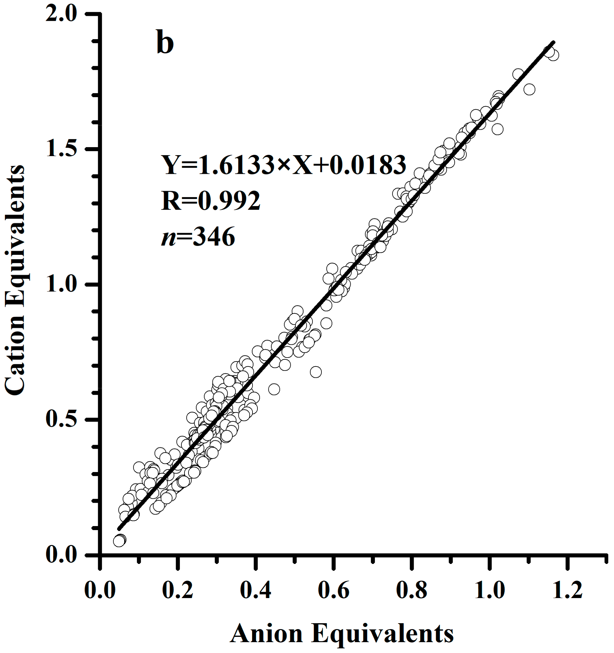
2.4. Ion Balance
2.5. Calculation of Secondary Organic Carbon (SOC)
2.6. NOR and SOR
2.7. PCA/APCS Receptor Model
3. Results and Discussion
3.1. Summary of the Haze Episode
3.2. Chemical Component Variations on Haze and non-Haze Days
3.3. Diurnal Variations of Pollutants
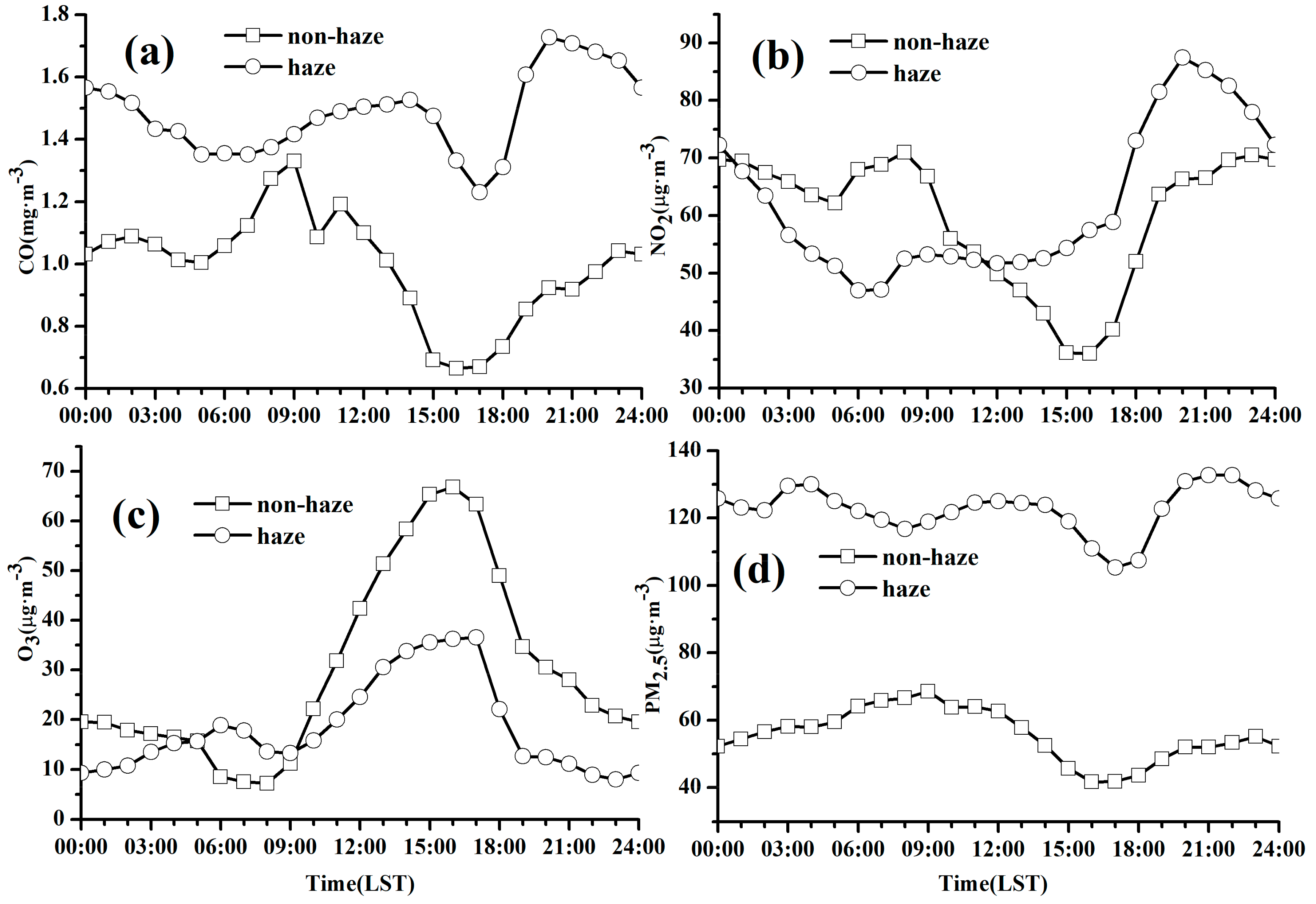
3.3.1. Diurnal Variations of PM2.5 and Trace Gases
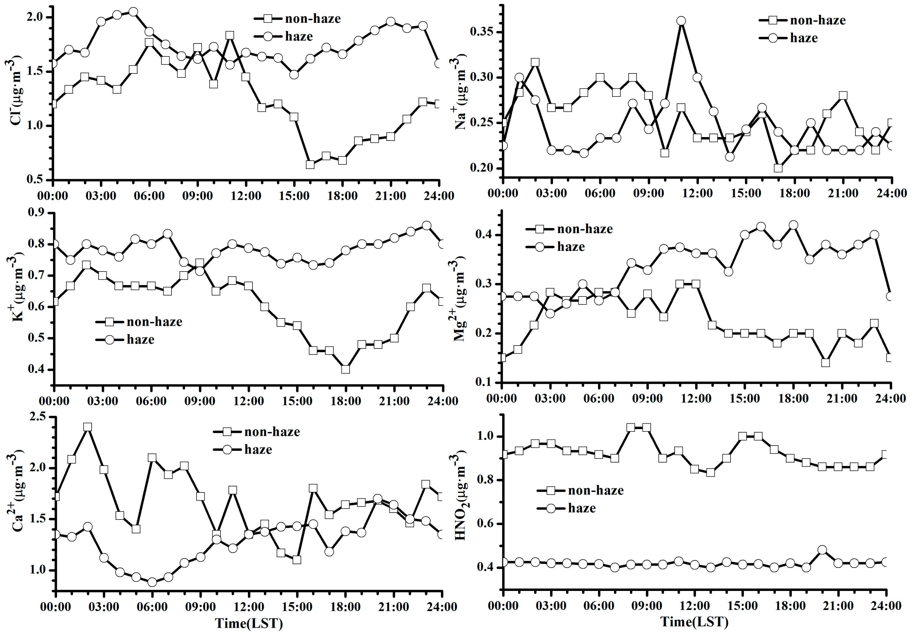
3.3.2. Diurnal Variations of Chemical Components
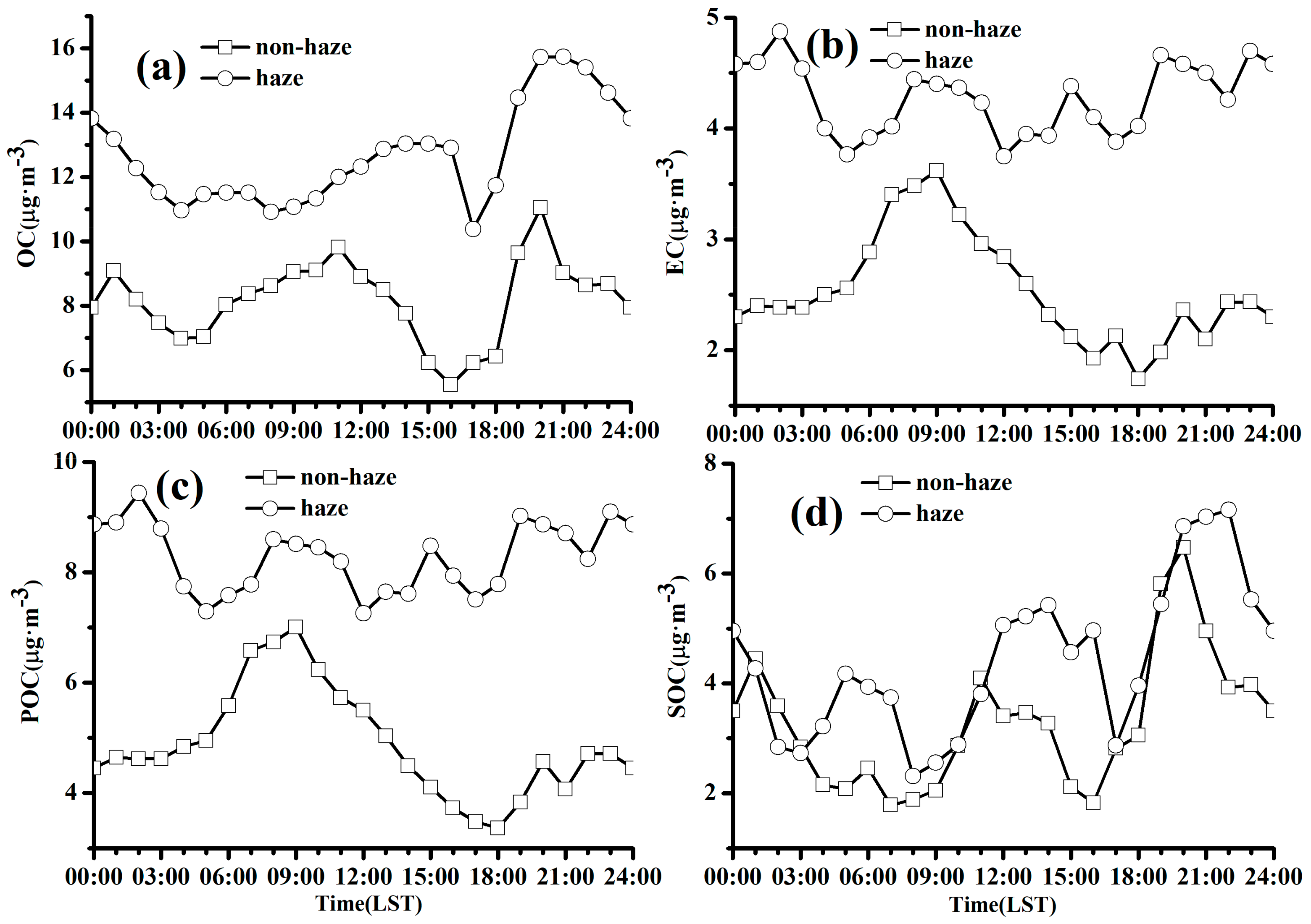
3.3.3. Diurnal Variation of Carbonaceous Aerosol
3.4. NOR and SOR
3.5. Source Apportionment of Pollutants
4. Conclusions
Author Contributions
Funding
Acknowledgments
Conflicts of Interest
References
- Huang, R.J.; Zhang, Y.; Bozzetti, C.; Ho, K.F.; Cao, J.J.; Han, Y.; Daellenbach, K.R.; Slowik, J.G.; Platt, S.M.; Canonaco, F.; et al. High secondary aerosol contribution to particulate pollution during haze events in China. Nature 2014, 514, 218–222. [Google Scholar] [CrossRef] [PubMed]
- Gao, J.; Woodward, A.; Vardoulakis, S.; Kovats, S.; Wilkinson, P.; Li, L.; Xu, L.; Li, J.; Yang, J.; Li, J.; et al. Haze, public health and mitigation measures in China: A review of the current evidence for further policy response. Sci. Total Environ. 2017, 578, 148–157. [Google Scholar] [CrossRef] [PubMed]
- Li, H.; Wu, H.; Wang, Q.; Yang, M.; Li, F.; Sun, Y.; Qian, X.; Wang, J.; Wang, C. Chemical partitioning of fine particle-bound metals on haze-fog and non-haze-fog days in Nanjing, China and its contribution to human health risks. Atmos. Res. 2017, 183, 142–150. [Google Scholar] [CrossRef]
- Shen, L.; Wang, H.; Lü, S.; Zhang, X.; Yuan, J.; Tao, S.; Zhang, G.; Wang, F.; Li, L. Influence of pollution control on air pollutants and the mixing state of aerosol particles during the 2nd world internet conference in Jiaxing, China. J. Clean. Prod. 2017, 149, 436–447. [Google Scholar] [CrossRef]
- Zhang, R.; Sun, X.; Shi, A.; Huang, Y.; Yan, J.; Nie, T.; Yan, X.; Li, X. Secondary inorganic aerosols formation during haze episodes at an urban site in Beijing, China. Atmos. Environ. 2018, 177, 275–282. [Google Scholar] [CrossRef]
- Xu, X.; Zhao, T.; Liu, F.; Gong, S.L.; Kristovich, D.; Lu, C.; Guo, Y.; Cheng, X.; Wang, Y.; Ding, G. Climate modulation of the Tibetan Plateau on haze in China. Atmos. Chem. Phys. 2016, 16, 1365–1375. [Google Scholar] [CrossRef]
- Zhao, H.; Zhang, X.; Zhang, S.; Chen, W.; Tong, D.; Xiu, A. Effects of agricultural biomass burning on regional haze in China: A review. Atmosphere 2017, 8, 88. [Google Scholar] [CrossRef]
- Che, H.; Zhang, X.; Li, Y.; Zhou, Z.; Qu, J.J. Horizontal visibility trends in China 1981–2005. Geophys. Res. Lett. 2007, 34, L24706. [Google Scholar] [CrossRef]
- Qin, K.; Wu, L.; Wong, M.; Letu, H.; Hu, M.; Lang, H.; Sheng, S.; Teng, J.; Xiao, X.; Yuan, L. Trans-boundary aerosol transport during a winter haze episode in China revealed by ground-based Lidar and CALIPSO satellite. Atmos. Environ. 2016, 141, 20–29. [Google Scholar] [CrossRef]
- Liao, Y.; Wu, X.; Pan, Z.; Zhao, F.; Zhu, Y.; Duan, L.; Li, C.; Li, Y.; Cui, W.; Li, Q. Climatic characteristics of haze in Hunan province during 1961–2006. Adv. Climate Change Res. 2007, 5, 260–265. [Google Scholar]
- Lu, M.; Tang, X.; Wang, Z.; Gbaguidi, A.; Liang, S.; Hu, K.; Wu, L.; Wu, H.; Huang, Z.; Shen, L. Source tagging modeling study of heavy haze episodes under complex regional transport processes over Wuhan megacity, central China. Environ. Poll. 2017, 231, 612–621. [Google Scholar] [CrossRef] [PubMed]
- Che, H.; Zhang, X.; Li, Y.; Zhou, Z.; Qu, J.J.; Hao, X. Haze trends over the capital cities of 31 provinces in China, 1981–2005. Theor. App. Climatol. 2009, 97, 235–242. [Google Scholar] [CrossRef]
- Sun, E.; Xu, X.; Che, H.; Tang, Z.; Gui, K.; An, L.; Lu, C.; Shi, G. Variation in MERRA-2 aerosol optical depth and absorption aerosol optical depth over China from 1980 to 2017. J. Atmos. Sol. Terr. Phy. 2019, 186, 8–19. [Google Scholar] [CrossRef]
- Zhao, T.; Liu, D.; Zheng, X.; Yang, L.; Gu, X.; Hu, J.; Shu, Z.; Chang, J.; Wu, X. Revealed variations of air quality in industrial development over a remote plateau of Southwest China: An application of atmospheric visibility data. Meteorol. Atmos. Phys. 2017, 129, 1–9. [Google Scholar] [CrossRef]
- Zhao, S.; Yu, Y.; Yin, D.; He, J.; Liu, N.; Qu, J.; Xiao, J. Annual and diurnal variations of gaseous and particulate pollutants in 31 provincial capital cities based on in situ air quality monitoring data from China national environmental monitoring center. Environ. Int. 2016, 86, 92–106. [Google Scholar] [CrossRef]
- Xu, X.; Wang, Y.; Zhao, T.; Cheng, X.; Meng, Y.; Ding, G. “Harbor” effect of large topography on haze distribution in eastern China and its climate modulation on decadal variations in haze. Chin. Sci. Bull. 2015, 60, 1132–1143. [Google Scholar] [CrossRef]
- Chen, Y.; Xie, S. Spatiotemporal pattern and regional characteristics of visibility in China during 1976–2010. Chin. Sci. Bull. 2014, 59, 3054–3065. [Google Scholar] [CrossRef]
- Su, T.; Xu, M.; Zhou, X.; Yang, Z.; Yuan, J.; Zhang, H. Study on the variation characteristics of haze weather in Hubei province during 1980–2012. Agr. Sci. Technol. 2015, 16, 176. [Google Scholar]
- Ma, D.; Li, L.; Ju, Y. Climate characteristics of haze days and analysis of summer haze weather event in Hubei province. Environ. Sci. Technol. 2015, 38, 148–153. [Google Scholar]
- Zhang, F.; Wang, Z.W.; Cheng, H.R.; Lv, X.P.; Gong, W.; Wang, X.M.; Zhang, G. Seasonal variations and chemical characteristics of PM2.5 in Wuhan, central China. Sci. Total Environ. 2015, 518, 97–105. [Google Scholar] [CrossRef]
- Chen, N.; Xu, K.; Cao, Z.; Liu, D.; Hu, H.; Quan, J.; Tian, Y.; Shen, F. Analysis on the pollution levels of atmospheric particles and the correlation of pollutants in Hubei province. Environ. Sci. Technol. 2016, 39, 194–198. [Google Scholar]
- Xiong, Y.; Zhou, J.; Schauer, J.J.; Yu, W.; Hu, Y. Seasonal and spatial differences in source contributions to PM2.5 in Wuhan, China. Sci. Total Environ. 2017, 577, 155–165. [Google Scholar] [CrossRef] [PubMed]
- Zhang, M.; Ma, Y.; Gong, W.; Zhu, Z. Aerosol optical properties of a haze episode in Wuhan based on ground-based and satellite observations. Atmosphere 2014, 5, 699–719. [Google Scholar] [CrossRef]
- Cheng, H.; Gong, W.; Wang, Z.; Zhang, F.; Wang, X.; Lv, X.; Liu, J.; Fu, X.; Zhang, G. Ionic composition of submicron particles (PM1.0) during the long-lasting haze period in January 2013 in Wuhan, central China. J. Environ. Sci. 2014, 26, 810–817. [Google Scholar] [CrossRef]
- Wang, H.; Shen, L.; Zhu, B.; Kang, H.; Hou, X.; Miao, Q.; Yang, Y.; Shi, S. Spatial and temporal distributions of air pollutants and size distribution of aerosols over central and Eastern China. Arch. Environ. Con. Tox. 2017, 72, 481–495. [Google Scholar] [CrossRef] [PubMed]
- Wu, J.; Zhang, P.; Yi, H.; Qin, Z. What causes haze pollution? An empirical study of PM2.5 concentrations in Chinese cities. Sustainability 2016, 8, 132. [Google Scholar] [CrossRef]
- Wang, C.; Wang, C.; Myint, S.W.; Wang, Z.H. Landscape determinants of spatio-temporal patterns of aerosol optical depth in the two most polluted metropolitans in the United States. Sci. Total Environ. 2017, 609, 1556–1565. [Google Scholar] [CrossRef] [PubMed]
- Guo, S.; Hu, M.; Zamora, M.; Peng, J.; Shang, D.; Zheng, J.; Du, Z.; Wu, Z.; Shao, M.; Zeng, L.; et al. Elucidating severe urban haze formation in China. Proc. Natl. Acad. Sci. USA 2014, 111, 17373–17378. [Google Scholar] [CrossRef] [PubMed]
- Hu, R.; Wang, H.; Yin, Y.; Chen, K.; Zhu, B.; Zhang, Z.; Kang, H.; Shen, L. Mixing state of ambient aerosols during different fog-haze pollution episodes in the Yangtze River Delta, China. Atmos. Environ. 2018, 178, 1–10. [Google Scholar] [CrossRef]
- Hu, R.; Wang, H.; Yin, Y.; Zhu, B.; Xia, L.; Zhang, Z.; Chen, K. Measurement of ambient aerosols by single particle mass spectrometry in the Yangtze River Delta, China: Seasonal variations, mixing state and meteorological effects. Atmos. Res. 2018, 213, 562–575. [Google Scholar] [CrossRef]
- Qiao, X.; Jaffe, D.; Tang, Y.; Bresnahan, M.; Song, J. Evaluation of air quality in Chengdu, Sichuan Basin, China: Are China’s air quality standards sufficient yet? Environ. Monit. Assess. 2015, 187, 250. [Google Scholar] [CrossRef] [PubMed]
- Wang, H.; Zhu, B.; Shen, L.; Xu, H.; An, J.; Pan, C.; Li, Y.; Liu, D. Regional characteristics of air pollutants during heavy haze events in the Yangtze River Delta, China. Aerosol Air Qual. Res. 2016, 16, 2159–2171. [Google Scholar] [CrossRef]
- Wang, Y.; Yao, L.; Wang, L.; Liu, Z.; Ji, D.; Tang, G.; Zhang, J.; Sun, Y.; Hu, B.; Xin, J. Mechanism for the formation of the January 2013 heavy haze pollution episode over central and eastern China. Sci. China Earth Sci. 2014, 57, 14–25. [Google Scholar] [CrossRef]
- He, K.; Zhao, Q.; Ma, Y.; Duan, F.; Yang, F.; Shi, Z.; Chen, G. Spatial and seasonal variability of PM2.5 acidity at two Chinese megacities: Insights into the formation of secondary inorganic aerosols. Atmos. Chem. Phys. 2012, 12, 25557–25603. [Google Scholar] [CrossRef]
- Wang, S.; Nan, J.; Shi, C.; Fu, Q.; Gao, S.; Wang, D.; Cui, H.; Saiz-Lopez, A.; Zhou, B. Atmospheric ammonia and its impacts on regional air quality over the megacity of Shanghai, China. Sci. Rep. 2015, 5, 15842. [Google Scholar] [CrossRef] [PubMed]
- Andrews, E.; Saxena, P.; Musarra, S.; Hildemann, L.M.; Koutrakis, P.; McMurry, P.H.; Olmez, I.; White, W.H. Concentration and composition of atmospheric aerosols from the 1995 SEAVS experiment and a review of the closure between chemical and gravimetric measurements. J. Air Waste Manage. 2000, 50, 648–664. [Google Scholar] [CrossRef]
- Du, H.; Kong, L.; Cheng, T.; Chen, J.; Du, J.; Li, L.; Xia, X.; Leng, C.; Huang, G. Insights into summertime haze pollution events over Shanghai based on online water-soluble ionic composition of aerosols. Atmos. Environ. 2011, 45, 5131–5137. [Google Scholar] [CrossRef]
- Chow, J.C.; Chen, L.W.A.; Watson, J.G.; Lowenthal, D.H.; Magliano, K.A.; Turkiewicz, K.; Lehrman, D.E. PM2.5 chemical composition and spatiotemporal variability during the California regional PM10/PM2.5 air quality study (CRPAQS). J. Geophys. Res. 2006, 111, D10S04. [Google Scholar] [CrossRef]
- Seinfeld, J.H.; Pandis, S.N. Atmospheric Chemistry and Physics: From Air Pollution to Climate Change, 2nd ed.; John Wiley & Sons: New York, NY, USA, 2006. [Google Scholar]
- Wang, Y.; Zhuang, G.S.; Zhang, X.Y.; Huang, K.; Xu, C.; Tang, A.H.; Chen, J.M.; An, Z.S. The ion chemistry, seasonal cycle, and sources of PM2.5 and TSP aerosol in Shanghai. Atmos. Environ. 2006, 40, 2935–2952. [Google Scholar] [CrossRef]
- Chen, S.J.; Liao, S.H.; Jian, W.J.; Lin, C.C. Particle size distribution of aerosol carbons in ambient air. Environ. Int. 1997, 23, 475–488. [Google Scholar] [CrossRef]
- Ji, D.; Zhang, J.; He, J.; Wang, X.; Pang, B.; Liu, Z.; Wang, L.; Wang, Y. Characteristics of atmospheric organic and elemental carbon aerosols in urban Beijing, China. Atmos. Environ. 2016, 125, 293–306. [Google Scholar] [CrossRef]
- Ding, A.J.; Huang, X.; Nie, W.; Sun, J.N.; Kerminen, V.-M.; Petäjä, T.; Su, H.; Cheng, Y.F.; Yang, X.-Q.; Wang, M.H.; et al. Enhanced haze pollution by black carbon in megacities in China. Geophys. Res. Lett. 2016, 43, 2873–2879. [Google Scholar] [CrossRef]
- Mauderly, J.L.; Chow, J.C. Health effects of organic aerosols. Inhal. Toxicol. 2008, 20, 257–288. [Google Scholar] [CrossRef]
- Jongejan, P.A.C.; Bai, Y.; Veltkamp, A.C.; Wyers, G.P.; Slanina, J. An automated field instrument for the determination of acidic gases in air. Int. Environ. An. Chem. 1997, 66, 241–251. [Google Scholar] [CrossRef]
- Chow, J.C.; Watson, J.G. Guideline on Speciated Particulate Monitoring; US Environmental Protection Agency: Reno, NV, USA, 1998; Volume 3–7, pp. 4–37. [Google Scholar]
- Khlystov, A.; Wyers, G.P.; Slanina, J. The steam-jet aerosol collector. Atmos. Environ. 1995, 29, 2229–2234. [Google Scholar] [CrossRef]
- Khezri, B.; Mo, H.; Yan, Z.; Chong, S.L.; Heng, A.K.; Webster, R.D. Simultaneous online monitoring of inorganic compounds in aerosols and gases in an industrialized area. Atmos. Environ. 2013, 80, 352–360. [Google Scholar] [CrossRef]
- Rumsey, I.C.; Cowen, K.A.; Walker, J.T.; Kelly, T.J.; Hanft, E.A.; Mishoe, K.; Rogers, C.; Proost, R.; Beachley, G.M.; Lear, G.; et al. An assessment of the performance of the monitor for AeRosols and GAses in ambient air (MARGA): A semi-continuous method for soluble compounds. Atmos. Chem. Phys. 2104, 14, 5639–5658. [Google Scholar] [CrossRef]
- Bae, M.S.; Schauer, J.J.; DeMinter, J.T.; Turner, J.R.; Smith, D.; Cary, R.A. Validation of a semi-continuous instrument for elemental carbon and organic carbon using a thermal-optical method. Atmos. Environ. 2004, 38, 2885–2893. [Google Scholar] [CrossRef]
- Bauer, J.J.; Yu, X.Y.; Cary, R.; Laulainen, N.; Berkowitz, C. Characterization of the sunset semi-continuous carbon aerosol analyzer. J. Air Waste Manage. Assoc. 2009, 59, 826–833. [Google Scholar] [CrossRef]
- Jiang, R.; Tan, H.; Tang, L.; Cai, M.; Yin, Y.; Li, F.; Liu, L.; Xu, H.; Chan, P.W.; Deng, X.; et al. Comparison of aerosol hygroscopicity and mixing state between winter and summer seasons in Pearl River Delta region, China. Atmos. Res. 2016, 169, 160–170. [Google Scholar] [CrossRef]
- Chow, J.C.; Watson, J.G.; Lu, Z.; Lowenthal, D.H.; Frazier, C.A.; Solomon, P.A.; Thuillier, R.H.; Magliano, K. Descriptive analysis of PM2.5 and PM10 at regionally representative locations during SJVAQS/AUSPEX. Atmos. Environ. 1996, 30, 2079–2112. [Google Scholar] [CrossRef]
- Turpin, B.J.; Huntzicker, J.J. Identification of secondary organic aerosol episodes and quantification of primary and secondary organic aerosol concentrations during SCAQS. Atmos. Environ. 1995, 29, 3527–3544. [Google Scholar] [CrossRef]
- Castro, L.M.; Harrison, R.M.; Smith, D.J.T. Carbonaceous aerosol in urban and rural European atmospheres: Estimation of secondary organic carbon concentrations. Atmos. Environ. 1999, 33, 2771–2781. [Google Scholar] [CrossRef]
- Thurston, G.D.; Spengler, J.D. A quantitative assessment of source contributions to inhalable particulate matter pollution in metropolitan Boston. Atmos. Environ. 1985, 19, 9–25. [Google Scholar] [CrossRef]
- Miller, S.L.; Anderson, M.J.; Daly, E.P.; Milford, J.B. Source apportionment of exposures to volatile organic compounds. I. Evaluation of receptor models using simulated exposure data. Atmos. Environ. 2002, 36, 3629–3641. [Google Scholar] [CrossRef]
- Guo, H.; Wang, T.; Simpson, I.J.; Blake, D.R.; Yu, X.M.; Kwok, Y.H.; Li, Y.S. Source contributions to ambient VOCs and CO at a rural site in eastern China. Atmos. Environ. 2004, 38, 4551–4560. [Google Scholar] [CrossRef]
- Stull, R.B. An Introduction to Boundary Layer Meteorology; Kluwer Acad.: Dordrecht, The Netherlands, 1988; pp. 665–670. [Google Scholar]
- Song, J.; Wang, Z.H.; Wang, C. Biospheric and anthropogenic contributors to atmospheric CO2 variability in a residential neighborhood of Phoenix, Arizona. J. Geophys. Res. 2017, 122, 3317–3329. [Google Scholar] [CrossRef]
- Wang, H.; Zhu, B.; Shen, L.; Kang, H. Size distributions of aerosol and water-soluble ions in Nanjing during a crop residual burning event. J. Environ. Sci. 2012, 24, 1457–1465. [Google Scholar] [CrossRef]
- Tao, J.; Gao, J.; Zhang, L.; Zhang, R.; Che, H.; Zhang, Z.; Lin, Z.; Jing, J.; Cao, J.; Hsu, S.C. PM2.5 pollution in a megacity of southwest China: Source apportionment and implication. Atmos. Chem. Phys. 2014, 14, 8679–8699. [Google Scholar] [CrossRef]
- Liu, B.; Song, N.; Dai, Q.; Mei, R.; Sui, B.; Bi, X.; Feng, Y. Chemical composition and source apportionment of ambient PM2. 5 during the non-heating period in Taian, China. Atmos. Res. 2016, 170, 23–33. [Google Scholar] [CrossRef]
- Swietlicki, E.; Puri, S.; Hansson, H.C.; Edner, H. Urban air pollution source apportionment using a combination of aerosol and gas monitoring techniques. Atmos. Environ. 1996, 30, 2795–2809. [Google Scholar] [CrossRef]
- Chang, Y.; Liu, X.; Deng, C.; Dore, A.J.; Zhuang, G. Source apportionment of atmospheric ammonia before, during, and after the 2014 APEC summit in Beijing using stable nitrogen isotope signatures. Atmos. Chem. Phys. 2016, 16, 11635–11647. [Google Scholar] [CrossRef]


| Component | Non-Haze Days | Haze Days | |||||||
|---|---|---|---|---|---|---|---|---|---|
| Average | SD | Median | Sample Times | Average | SD | Median | Sample Times | ||
| Gas | CO (mg·m−3) | 0.99 | 0.30 | 1.05 | 161 h | 1.48 | 0.46 | 1.39 | 217 h |
| NO2 (μg·m−3) | 59.30 | 21.68 | 65.50 | 161 h | 61.85 | 19.39 | 57.00 | 217 h | |
| SO2 (μg·m−3) | 13.64 | 8.42 | 11.00 | 161 h | 10.56 | 7.19 | 8.00 | 217 h | |
| O3 (μg·m−3) | 30.32 | 24.23 | 20.00 | 161 h | 18.60 | 16.83 | 12.00 | 217 h | |
| HCl (μg·m−3) | 0.27 | 0.05 | 0.30 | 145 h | 0.25 | 0.07 | 0.30 | 156 h | |
| HNO2 (μg·m−3) | 0.92 | 0.38 | 1.20 | 145 h | 0.55 | 0.05 | 0.40 | 156 h | |
| HNO3 (μg·m−3) | 0.50 | 0.12 | 0.50 | 145 h | 0.67 | 0.13 | 0.60 | 156 h | |
| NH3 (μg·m−3) | 2.85 | 1.53 | 2.70 | 145 h | 6.23 | 2.20 | 5.90 | 156 h | |
| PM2.5 | PM2.5 (μg·m−3) | 55.78 | 19.63 | 58.00 | 161 h | 122.61 | 37.95 | 117.50 | 217 h |
| WSI | Cl- (μg·m−3) | 1.25 | 0.61 | 1.20 | 145 h | 1.75 | 0.84 | 1.60 | 156 h |
| NO3− (μg·m−3) | 8.22 | 4.43 | 7.80 | 145 h | 20.87 | 7.52 | 23.75 | 156 h | |
| SO42− (μg·m−3) | 5.13 | 4.37 | 4.60 | 145 h | 11.20 | 5.43 | 11.10 | 156 h | |
| Na+ (μg·m−3) | 0.26 | 0.07 | 0.30 | 145 h | 0.25 | 0.10 | 0.20 | 156 h | |
| NH4+ (μg·m−3) | 6.47 | 4.18 | 6.10 | 145 h | 16.07 | 7.20 | 17.80 | 156 h | |
| K+ (μg·m−3) | 0.61 | 0.28 | 0.60 | 145 h | 0.78 | 0.19 | 0.80 | 156 h | |
| Mg2+ (μg·m−3) | 0.23 | 0.13 | 0.20 | 145 h | 0.34 | 0.18 | 0.30 | 156 h | |
| Ca2+ (μg·m−3) | 1.68 | 0.87 | 1.90 | 145 h | 1.29 | 0.79 | 1.00 | 156 h | |
| Carbonaceous Aerosol | OC (μg·m−3) | 8.18 | 2.70 | 8.10 | 140 h | 12.66 | 2.60 | 12.20 | 134 h |
| EC (μg·m−3) | 2.54 | 0.97 | 2.70 | 140 h | 4.27 | 0.87 | 4.50 | 134 h | |
| POC (μg·m−3) | 4.89 | 1.89 | 5.23 | 140 h | 8.25 | 1.68 | 8.71 | 134 h | |
| SOC (μg·m−3) | 3.29 | 1.86 | 2.97 | 140 h | 4.41 | 2.84 | 3.41 | 134 h | |
| Compounds | Non-Haze Days | Haze Days | ||||
|---|---|---|---|---|---|---|
| KMO = 0.775 | KMO = 0.592 | |||||
| FC1 | FC2 | FC3 | FC1 | FC2 | FC3 | |
| CO | 0.34 | 0.15 | 0.75 | 0.44 | −0.21 | 0.72 |
| NO2 | −0.05 | 0.34 | 0.85 | −0.12 | 0.20 | 0.88 |
| SO2 | 0.29 | 0.70 | 0.24 | −0.46 | 0.61 | 0.46 |
| Cl− | 0.53 | 0.48 | 0.45 | 0.81 | 0.00 | 0.04 |
| NO3- | 0.86 | 0.39 | 0.13 | 0.89 | −0.17 | −0.25 |
| SO42− | 0.85 | −0.07 | 0.20 | 0.89 | −0.22 | 0.04 |
| NH3 | 0.66 | 0.54 | 0.08 | 0.44 | 0.20 | −0.49 |
| Na+ | 0.10 | 0.65 | 0.41 | −0.18 | 0.81 | −0.12 |
| NH4+ | 0.95 | 0.12 | 0.18 | 0.94 | −0.26 | −0.11 |
| K+ | 0.68 | 0.53 | 0.37 | 0.84 | 0.30 | 0.01 |
| Mg2+ | 0.24 | 0.81 | 0.08 | 0.26 | 0.72 | 0.02 |
| Ca2+ | −0.02 | 0.75 | 0.35 | −0.20 | 0.79 | 0.43 |
| OC | 0.26 | 0.19 | 0.78 | 0.07 | 0.41 | 0.62 |
| EC | 0.55 | 0.36 | 0.66 | 0.63 | 0.06 | 0.37 |
| Initial eigenvalue | 7.62 | 1.89 | 1.19 | 5.25 | 3.19 | 1.77 |
| % of variance | 54.44 | 13.48 | 8.48 | 37.52 | 22.77 | 12.66 |
| Cumulative % | 54.44 | 67.92 | 76.40 | 37.52 | 60.29 | 72.94 |
© 2019 by the authors. Licensee MDPI, Basel, Switzerland. This article is an open access article distributed under the terms and conditions of the Creative Commons Attribution (CC BY) license (http://creativecommons.org/licenses/by/4.0/).
Share and Cite
Gao, Z.; Wang, X.; Shen, L.; Xiang, H.; Wang, H. Observation and Source Apportionment of Trace Gases, Water-Soluble Ions and Carbonaceous Aerosol During a Haze Episode in Wuhan. Atmosphere 2019, 10, 397. https://doi.org/10.3390/atmos10070397
Gao Z, Wang X, Shen L, Xiang H, Wang H. Observation and Source Apportionment of Trace Gases, Water-Soluble Ions and Carbonaceous Aerosol During a Haze Episode in Wuhan. Atmosphere. 2019; 10(7):397. https://doi.org/10.3390/atmos10070397
Chicago/Turabian StyleGao, Zhengxu, Xiaoling Wang, Lijuan Shen, Hua Xiang, and Honglei Wang. 2019. "Observation and Source Apportionment of Trace Gases, Water-Soluble Ions and Carbonaceous Aerosol During a Haze Episode in Wuhan" Atmosphere 10, no. 7: 397. https://doi.org/10.3390/atmos10070397
APA StyleGao, Z., Wang, X., Shen, L., Xiang, H., & Wang, H. (2019). Observation and Source Apportionment of Trace Gases, Water-Soluble Ions and Carbonaceous Aerosol During a Haze Episode in Wuhan. Atmosphere, 10(7), 397. https://doi.org/10.3390/atmos10070397