Article

Historical Winter Storm Atlas for Germany (GeWiSA)

Environmental Meteorology, Albert-Ludwigs-University of Freiburg, Werthmannstrasse 10, D-79085 Freiburg, Germany
*
Author to whom correspondence should be addressed.
Atmosphere 2019, 10(7), 387; https://doi.org/10.3390/atmos10070387
Submission received: 31 May 2019 / Revised: 28 June 2019 / Accepted: 8 July 2019 / Published: 11 July 2019
(This article belongs to the Section Meteorology)

Abstract

:
Long-term gust speed (GS) measurements were used to develop a winter storm atlas of the 98 most severe winter storms in Germany in the period 1981–2018 (GeWiSa). The 25 m × 25 m storm-related GS fields were reconstructed in a two-step procedure: Firstly, the median gust speed ( G S ˜ ) of all winter storms was modeled by a least-squares boosting (LSBoost) approach. Orographic features and surface roughness were used as predictor variables. Secondly, the quotient of GS related to each winter storm to G S ˜ , which was defined as storm field factor (STF), was calculated and mapped by a thin plate spline interpolation (TPS). It was found that the mean study area-wide GS associated with the 2007 storm Kyrill is highest (29.7 m/s). In Southern Germany, the 1999 storm Lothar, with STF being up to 2.2, was the most extreme winter storm in terms of STF and GS. The results demonstrate that the variability of STF has a considerable impact on the simulated GS fields. Event-related model validation yielded a coefficient of determination (R2) of 0.786 for the test dataset. The developed GS fields can be used as input to storm damage models representing storm hazard. With the knowledge of the storm hazard, factors describing the vulnerability of storm exposed objects and structures can be better estimated, resulting in improved risk management.

1. Introduction

Strong storms chronically lead to enormous socio-economic damage [1]. In the period 1981–2018, storm events around the world caused total losses of about US$ 2115bn and led to approximately 446,000 fatalities [1]. The spatiotemporal extent of storm events greatly varies depending on the geographical location and the time during the year [2]. In Central Europe, storm events can roughly be classified into two categories: small-scale thunderstorms, which mainly occur from May to September [3,4,5,6], and large-scale winter storms mainly occurring from October to March, which are related to intense low-pressure systems [2,7,8,9,10]. As a part of Central Europe, Germany was often hit by severe winter storms, causing total losses of about US$ 37bn and 300 fatalities since 1981 [1].
The most destructive feature of winter storms are high-impact gusts, which are short-time fluctuations of the horizontal wind vector [11,12]. High gust speed (GS) seriously affects numerous sectors including forestry [13,14,15], insurance [16], local authorities [17], wind energy [2], waterways transport [18] and air traffic [19]. In these sectors, there is great interest in spatially explicit modeled GS fields for improving the identification of storm damage risk factors [15].
Among the approaches used to model storm characteristics including GS, mechanistic models [7,8] can be differentiated from statistical (empirical) models [20,21,22,23]. Mechanistic models are useful tools for characterizing and investigating physical processes that determine storm formation, storm life cycle and storm-related GS dynamics. However, one of the major challenges in the application of mechanistic models is the knowledge of and the control over the large number of input parameters and the rather extensive initialization as well as parameterization for particular datasets.
The second, widely used approach is statistical (empirical) modeling, which is based on measured GS values. Although statistical approaches provide only general insights into the physical mechanisms of GS dynamics, they can be applied to assess GS field dynamics associated with winter storms. However, due to measurement errors, missing data and low temporal resolution, the quality of many GS time series is poor [24]. Comprehensive preparation is usually a basic prerequisite for the scientific analysis and interpretation of GS data. This mostly includes breakpoint analysis, measurement height correction and gap filling [25]. Moreover, long-term GS measurements are rare [26]. The small number of high-quality GS time series is a serious issue, since GS is one of the fastest varying atmospheric variables [27]. Complex land cover pattern and orographic obstacles at and around GS measuring sites further reduce the spatial representativeness of the few available long-term GS measurements [28,29].
To improve the spatial representativeness, statistical approaches making use of relationships between surface properties and GS were applied to model GS on high spatial resolution grids. For instance, the 98th percentiles of daily maximum GS time series were modeled for Switzerland on a 50 m × 50 m resolution grid [20]. Return periods of extreme GS were mapped in Germany on a 1000 m × 1000 m resolution grid [21]. In another study, 69 GS time series were used to model GS distributions on a 50 m × 50 m resolution grid in Southwestern Germany [22]. Using terrain and roughness-related information as predictor variables (PV), storm event-related GS was modeled on a 50 m × 50 m grid in Southwest Germany [23].
The above-mentioned studies investigated either the statistical properties of GS distributions or individual storm events. Since all storms have a unique track, the results of these studies are either not related to a particular storm event or individual showcases. To combine both approaches, it is necessary to consider the tracks of many storms in the statistical modeling of GS. This allows improved statements to be made about the spatiotemporal GS variability and the associated storm damage. The combined analysis of many storm events allows not only statements about central tendencies of GS during storms, but also about the deviation of individual storm events from the central tendencies.
Considering these aspects, the goals of this study are (1) reconstructing the storm fields associated with the most destructive winter storms in Germany in the period 1981–2018 and (2) high-spatial resolution modeling of GS associated with these storms. The mapping of the GS fields yields the winter storm atlas for Germany (GeWiSA).

2. Material and Methods

2.1. Overview

The development of GeWiSA comprises the following main steps (Figure 1): (1) obtaining a GS time series of 307 measurement stations operated by the German Meteorological Service (DWD) in the period 1981–2018, (2) breakpoint analysis and correction of GS time series, (3) extraction of GS associated with the 98 most destructive winter storms, (4) calculation of median GS ( G S ˜ ), (5) calculation of the storm field factor (STF), (6) estimation of roughness length (z0), (7) assessment of relative elevation (η) and orographic sheltering (σ), (8) modeling of GS based on a LSBoost approach and PV, (9) thin plate spline interpolation (TPS) of STF, (10) multiplication of G S ˜ by STF yielding GS.

2.2. Study Area and Evaluated Winter Storms

Germany has a size of about 357,000 km². The German landscape consists of four large natural areas: the North German Plain, the Central German Plain, the Alpine Foothills and the Alps in Southern Germany [30]. Germany’s surface is covered by agricultural areas (59%), forests (30%) and artificial surfaces such as urban areas, airports and road and rail networks (8%) [30,31].
In total, 98 severe winter storms were included in GeWiSA (Table 1). The storms were selected based on the overall losses (inflation-adjusted 2018 $) from Munich Re’s NatCatSERVICE [1]. The first winter storm contained in Munich Re’s NatCatSERVICE occurred in 1981. A maximum number of five severe winter storms per year was selected with overall losses being at least US$ 3.0m. According to the overall losses, the most severe storms were Kyrill (US$ 5100 m), Lothar (US$ 2200m) and Friederike (US$ 1900 m) [1]. A year with several severe winter storms was 1990. In this year, storms Daria, Vivian and Wiebke occurred, causing US$ 1800 m each.

2.3. Gust Speed (GS) Data

Maximum daily GS including all measurements available from the DWD climate data center in the period 1981–2018 was used for GeWiSA development [32]. Based on the data availability (DA), GS time series were included in the parameterization dataset (DS1) and test dataset (DS2). DS1 contains 135 GS time series with DA > 90.0% (Figure 2). DS2 contains 172 GS time series with DA being in the range 25.0–89.9%. Time series where DA < 25.0% were not considered for further analysis.
Due to the long measurement period, the metadata revealed numerous GS station relocations, measuring height changes and/or instrument changes [22]. To use homogenous GS time series, a breakpoint analysis was carried out for each GS time series, and, if necessary, the GS time series was corrected by quantile matching [22,33,34].

2.4. Predictor Variables (PV)

A total of 37 PVs that are known to influence GS [22,23,25] were developed to model the spatial GS pattern at 25 m × 25 m resolution. One PV was the measuring height of GS (h), which is often (47%), but not always, 10 m above ground level as recommended by the World Meteorological Organization. To consider the large-scale pattern of GS, longitude (lon) and latitude (lat) were used as PVs (Table 2). Esri’s ArcGIS® 10.4 software (Redlands, CA, USA) was used for PV building.
All orographic PVs were derived from the digital elevation model EU-DEM v.1 [35]. The elevation (ε) was rescaled from the original 20 m × 20 m to 25 m × 25 m using ArcGIS’ aggregate tool. Based on ε, the relative elevation (η) was calculated by subtracting the mean elevation of an outer circle of each grid cell from the grid cell-specific ε value [24]. Four η variants with outer-circle radii of 1000 m (η1000), 3000 m (η3000), 5000 m (η5000) and 7500 m (η7500) were built. For the eight main compass directions, η was modeled with a 3000 m radius. Another PV for describing the orography was sheltering (σ), which was also calculated for the eight main compass directions by summing up the angles between grid cell-specific elevation and the visible horizon up to a distance of 1000 m [36].
The z0-related predictors originate from the European Settlement Map (ESM) 2012 R 2017 [37]. The ESM 2012 R 2017 data set contains highly resolved 2.5 m × 2.5 m grid cells and their land use classes. First, a z0 value was assigned to each land use class (Table 3) [38]. Then, the 2.5 m × 2.5 m z0 grid was aggregated to 25 m × 25 m. For the eight main compass directions effective z0 was calculated in a 400 m radius to account for non-local roughness-induced modification of GS [25].

2.5. LS-Boost Modeling (LSBoost)

The spatial median gust speed pattern at 25 m × 25 m was modeled by the LSBoost algorithm [36] which is implemented in the Matlab® Software Statistics and Machine Learning Toolbox (Release 2018b; The Math Works Inc., Natick, MA, USA). The LSBoost model is a sequence of regression trees (B), i.e., decision trees with binary splits for regression. It aims at reducing the mean squared error (MSE) between G S ˜ and the aggregated G S ˜ prediction ( G S ^ ) of B [39,40,41]. The algorithm starts by calculating the median of G S ˜ ( G S ˜ ) of all DS1 stations. Then, the regression trees B1, …, Bm are combined in a weighted manner [39,40,41] to improve model accuracy. The individual regression trees are a function of selected PV:
G S ^ ( P V ) = G S ˜ ( P V ) + v m = 1 M p m B m ( P V )
where pm is the weight for model m, M is the total number of regression trees, and 0 < v ≤ 1 is the learning rate [39,40,41].
The number of PVs available for modeling G S ˜ enabled more than 3400 combinations (PVC), with different number of PVs to be evaluated and sorted in descending order according to the coefficient of determination ( R 2 ) related to DS2 ( R D S 2 2 ). Averaging the three first PVC yielded the overall highest R D S 2 2 . Thus, the first three PVC were used for development of the final G S ˜ map.

2.6. Thin Plate Spline Interpolation (TPS)

The quotient of GS related to a specific storm event to G S ˜ is STF, which describes the gust speed intensity:
S T F = G S G S ˜
which was modeled by a thin plate spline interpolation [42] in the entire study area. The applied TPS algorithm is implemented in the Matlab® Software Curve Fitting Toolbox (Release 2018b; The Math Works Inc., Natick, MA, USA). Geographic information from lon and lat were used as predictors for STF estimation. Multiplication of modeled G S ˜ by STF yielded the storm-related GS.

3. Results and Discussion

3.1. Median Gust Speed

In Table 4, three PVC consisting of seven PVs each are listed. Besides lon, lat and h, which were used in all models, PVC from SW and S sectors was used. One reason for including directional information on η, σ and z0 is that the main wind direction during winter storms is southwest [43]. It is striking that elevation was not included in the most informative models.
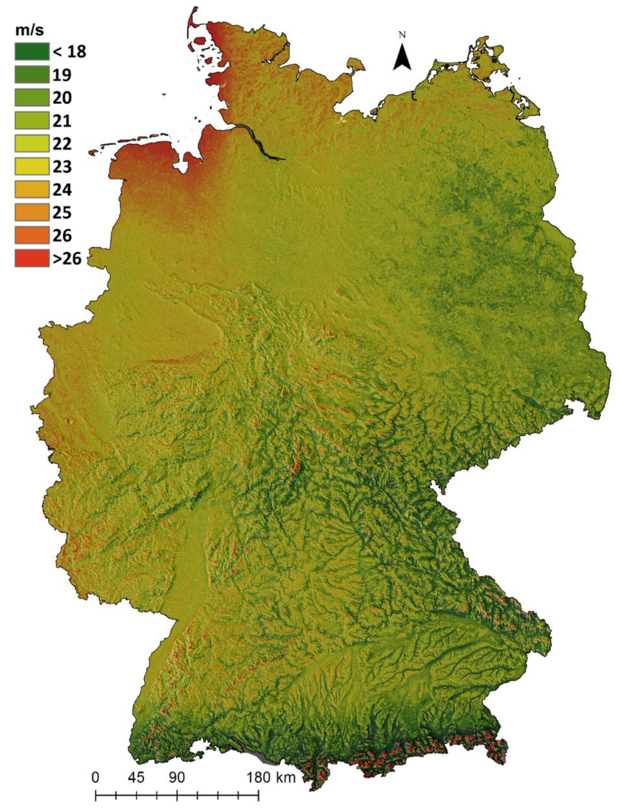
The G S ˜ field in h = 10 m related to severe winter storms is presented in Figure 3. Highest G S ˜ values can be found in the northwestern parts of the study area. Close to the North Sea coast and on the offshore islands, G S ˜ is up to 27 m/s. Lowest G S ˜ values occur in the south. There, G S ˜ is often below 20 m/s. Reasons for the decreasing GS values towards the southern lowlands are the increasing surface roughness, the increasing distance from the coast and the more complex orography, i.e., sheltering, in southern Germany. There is also a slight decreasing G S ˜ tendency from west to east. While G S ˜ in the west is about 23 m/s, in the east it is close to 20 m/s. Despite the large-scale G S ˜ pattern, very high G S ˜ values occur in low mountain ranges on mountain tops throughout the study area. In some places, G S ˜ even exceeds the G S ˜ values near the coasts. However, this is only the case where η7500 ≥ 350 m and σsum ≤ 80°. In contrast, lowest G S ˜ (< 15 m/s) were mainly simulated in the strongly incised valleys where η7500 ≤ −300 m and σsum ≥ 300°. The effect of z0 on G S ˜ is weaker, but it leads to lower G S ˜ in urban and forested areas.
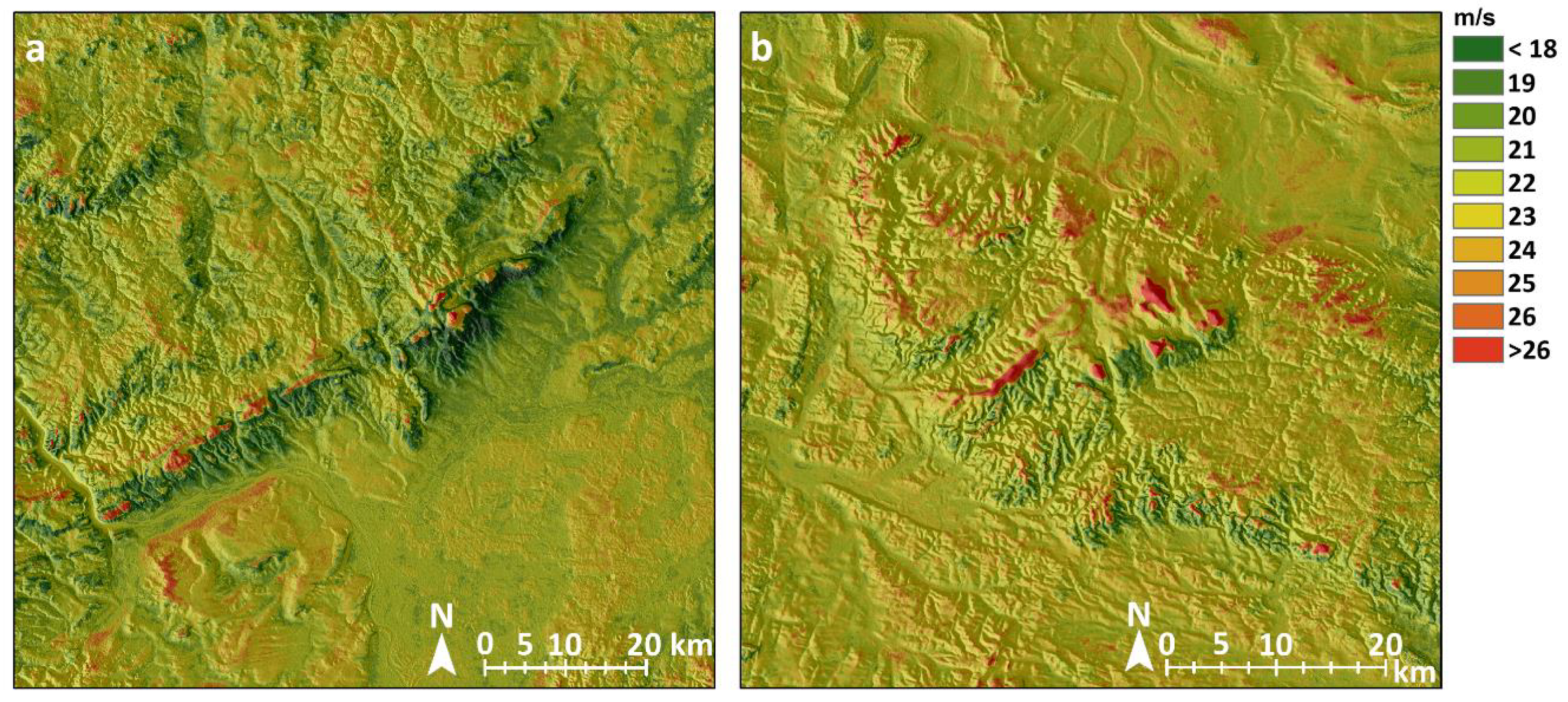
To illustrate the small-scale G S ˜ variability, two map extracts in complex terrain are presented in Figure 4. In the center of the first map extract is the southwest-northeast oriented mountain range Taunus located north of the city of Frankfurt (Figure 4a). The highest G S ˜ value (32 m/s) is simulated close to a mountaintop due to the exceptional combination of η7500 = 293 m, σsum = 147° and z0,sw = 87 mm. In eastern direction, in a distance of less than 2 km from the mountain top, G S ˜ is below 18 m/s which is mainly due to high σsum > 250° and z0,sw = 750 mm.
The second map extract shows the region around the Brocken (Figure 4b). The Brocken (1141 m a.s.l.) is an exposed mountain top, where chronically very high wind speeds occur [30] and G S ˜ = 37 m/s is also very high. This is because of the extraordinary exposure of η7500 > 400 m and z0,sw < 100 mm. However, areas with very low G S ˜ values can be found in close vicinity of the highest G S ˜ values. For example, 800 m east of Brocken’s summit G S ˜ is only 22 m/s.

3.2. Storm Field Factor (STF)

In Figure 5, STF is presented for four severe storms that caused the highest losses in Germany in the study period. STF values related to storm Daria (25–26 January 90) are high (up to 2.0) in the northwest of Germany (Figure 5a). In the east and southeast of the study area, Daria was much less intense with STF < 1.0. In contrast, storm Lothar (26 December 99) was exceptionally strong in Southern Germany (Figure 5b) with STF values up to 2.2. Central and northern parts of the study area were not hit by Lothar with STF < 1.0 over wide areas. Although GS associated with storm Kyrill (18–19 January 2007) is greater than G S ˜ over almost entire Germany (Figure 5c), the highest STF values (2.1) are lower compared to the highest Lothar-related STF values. Similar to storm Lothar, storm Friederike (18 January 18) hit a compact zone with only a few fringes to the south (Figure 5d). In the entire north of the study area, STF < 1.0. The study area-wide maximum STF value is 1.6 occurring in Central Germany. Overall, STF values in the study area are lower than those related to the other displayed winter storms.
If a large STF variability occurs at a small spatial distance, it is likely that two or more measuring stations in the immediate vicinity have a very different gust speed intensity. In such a case, the great stochastic component of gusts becomes apparent.
The representation of storm-related GS intensity by STF makes it very clear that GS is highly storm-specific. On the other hand, the common reference, i.e., G S ˜ , allows a consistent (1) assessment across all analyzed storm events, (2) comparison of the gust speed intensity of all analyzed storm events and (3) delimitation of all analyzed storm events. Furthermore, the separation of GS into G S ˜ and STF enables a simplified model building for GS associated with future storms, because only STF needs to be modeled. Using this approach, synthetic GS fields can easily be produced.
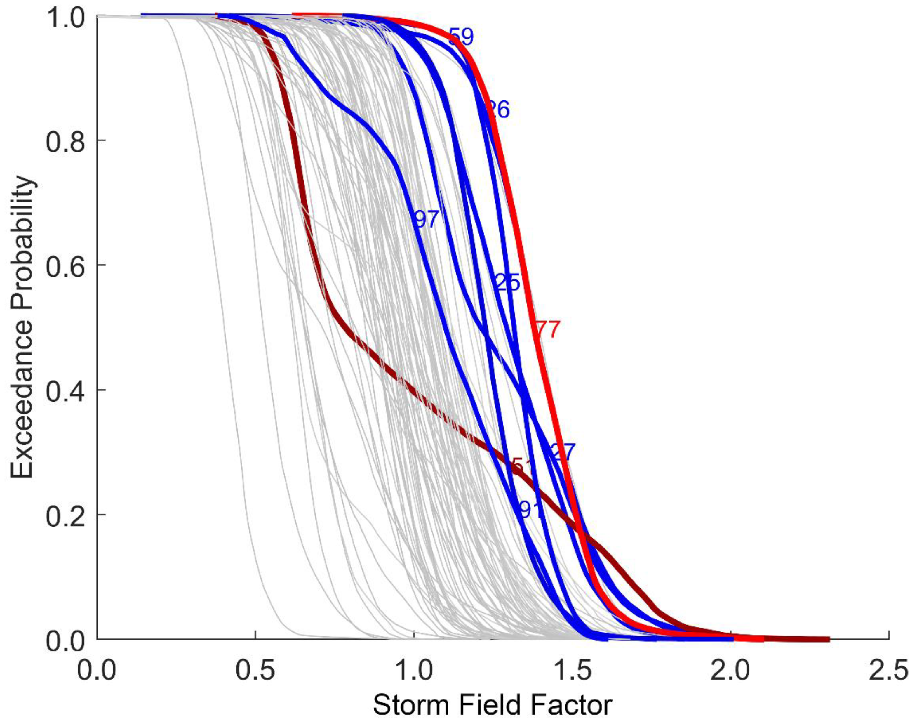
Since STF is derived as a deviation from the common reference G S ˜ for all storms, it is possible to consistently determine and compare the share of the study area where STF exceeds a certain value. Here, the comparison of all analyzed storm events is presented by survival functions (SF) of STF (Figure 6). Survival functions represent the exceedance probability of STF in the study area. Accordingly, storm Kyrill exceeds G S ˜ on the largest part of the study area. The median STF ( S T F ˜ ) for Kyrill is 1.38. On 5% of the study area, Kyrill-specific STF > 1.63. For storm Lothar, S T F ˜ = 0.79 and for storm Daria, S T F ˜ = 1.29. Comparing the distribution of S T F , Kyrill’s storm field extends over a much larger area than the storm fields of all other storms.
The shape of SF related to storm Lothar differs greatly from most other SFs. On the upper tail of SF, where the exceedance probability is below 0.05, storm Lothar (STF = 1.76) is very exceptional. In the same exceedance probability range, STF of storm Daria is 1.62. In contrast, STF values related to storm Friederike are much smaller ( S T F ˜ = 1.01). The great amount of damage caused by storm Friederike can be explained by the fact that its storm field hit several densely populated regions.

3.3. Winter Storm-Related Gust Speed

The GS maps created from multiplying G S ˜ by STF are displayed in Figure 7. For storm Daria, a clear northwest-southeast gradient of GS was modeled (Figure 7a). In large parts of Northwestern Germany, GS is in the range 30–40 m/s. Apart from exposed mountain tops, GS ≈ 20 m/s in the southeast. During storm Lothar, GS in Northern Germany is often below 15 m/s (Figure 7b) whereas in a clearly defined area in Southern Germany GS often exceeds 25 m/s. In some areas, GS even exceeds 50 m/s. Storm Kyrill hit Germany with an extensive high-impact gust speed field (Figure 7c) with GS > 30 m/s frequently occuring in the study area and GS > 40 m/s over large areas in the west and southeast. The GS field of storm Friederike is most pronounced in Central Germany (Figure 7d). There, GS often exceeds 30 m/s. Also in the south, GS values are often at 20 m/s. In the north, GS values are relatively low (< 15 m/s). In contrast to the other three presented storms, there is no contiguous area where GS > 40 m/s.
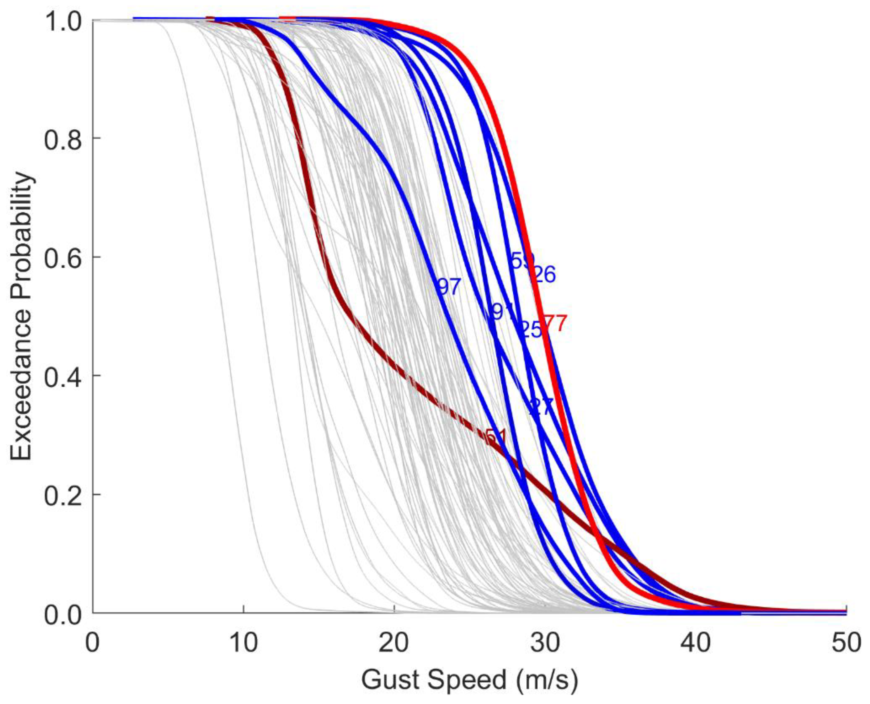
SFs of GS are presented in Figure 8. For storm Kyrill, the median is highest (29.7 m/s). A similarly high median value was modeled for storm Daria (27.9 m/s). In contrast, the median GS of Lothar is initially clearly lower (17.9 m/s). From the median on, however, SF belonging to Lothar cuts all other SFs. At exceedance probability 0.05 GS related to Lothar is 38.0 m/s. Moreover, for storm Daria GS is very high (37.0 m/s). Somewhat lower GS values occur for storm Kyrill (35.4 m/s) and especially storm Friederike (32.5 m/s). During storm Friederike, GS values of more than 34.4 m/s occur on 1% in the study area. The only storm where GS > 40 m/s at exceedance probability 0.01 is Lothar (42.8 m/s). The corresponding GS values for storms Daria (39.9 m/s), Kyrill (35.4 m/s) and Friederike (34.4 m/s) are considerably lower.
In general, SFs for GS and STF are very similar. However, the comparison of SFs for GS and STF related to a certain winter storm allows to draw conclusions about the absolute GS level and about the GS level in comparison to G S ˜ . For instance, winter storm Lothar’s STF survival function is well above all other SF for an exceedance probability < 0.20. In contrast, the SF for GS in the same exceedance probability range is only slightly above the other SF. This means that Lothar’s GS intensity was more extreme than its absolute GS level.

3.4. Model Comparison

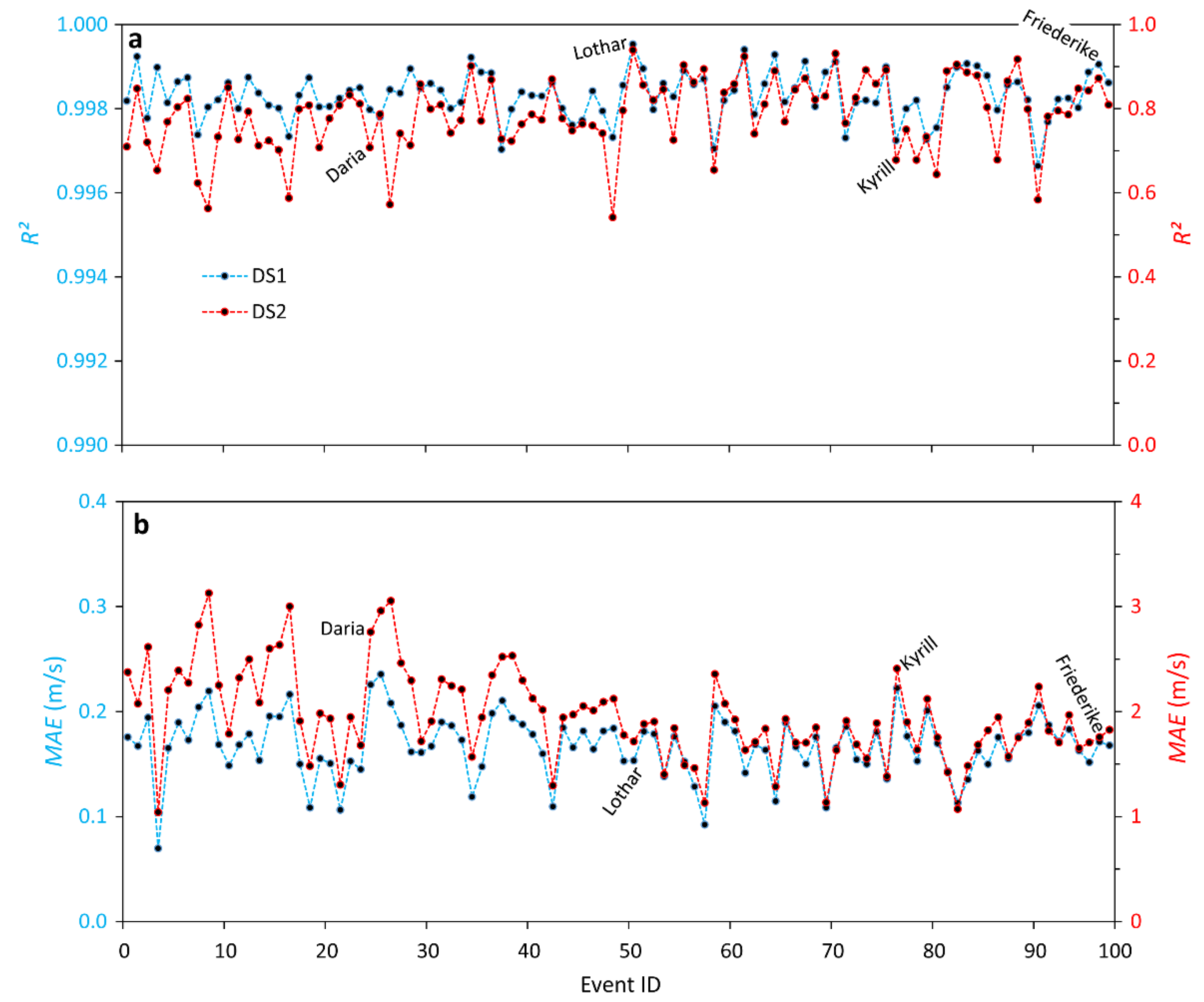
Results from comparing measured and modeled GS according to R2 are presented in Figure 9a for DS1 and DS2 (please note the different scaling of the y-axes). For DS1 mean R2 of all events is 0.998. The R2 standard deviation in DS1 is very low (0.001). For DS2, which is used to validate the model, mean R D S 2 2 is 0.786. A Mann-Kendall trend test revealed a significant (significance level: 0.05) trend of the R D S 2 2 values. The increasing model accuracy towards the end of the investigation period can be explained by the increasing number of GS time series available for model validation. The average data availability of DS2 before 1999 is 50%. From 1999, it is on average 61%. The data available for model parameterization in DS1 is about 97% for the entire period.
The highest R2 values ( R D S 1 2 = 1.000, R D S 2 2 = 0.939) were calculated for storm Lothar. One reason for this is the spatially clearly defined storm field. For all other storms, the deviation between R D S 1 2 and R D S 2 2 is clearly greater, e.g., for storm Kyrill R D S 1 2 = 0.997 and R D S 2 2 = 0.678. Based on all simulated GS fields, there is an indication that the standard deviation of GS in the study area is an important factor for storm event-related R 2 , correlation coefficient between standard deviation of GS and R 2 is 0.61 (significance level: < 0.00001), and thus for model accuracy. Starting with storm Lothar (ID: 51) in 1999, R D S 1 2 and R D S 2 2 have very similar variations, with mean R 2 being the only distinctive feature.
The second model accuracy measure is mean absolute error (MAE) (Figure 9b). For DS1, mean MAEDS1 is 0.17 m/s, which is within the typical GS measurement accuracy. Moreover, there is no temporal trend in MAEDS1. This does not apply for DS2, where mean MAEDS2 for all events before storm Lothar is 2.2 m/s. After 1999 MAEDS2 = 1.7 m/s.
From the presented error measures it is concluded that the simulated GS fields very reasonably reconstruct historical GS fields.
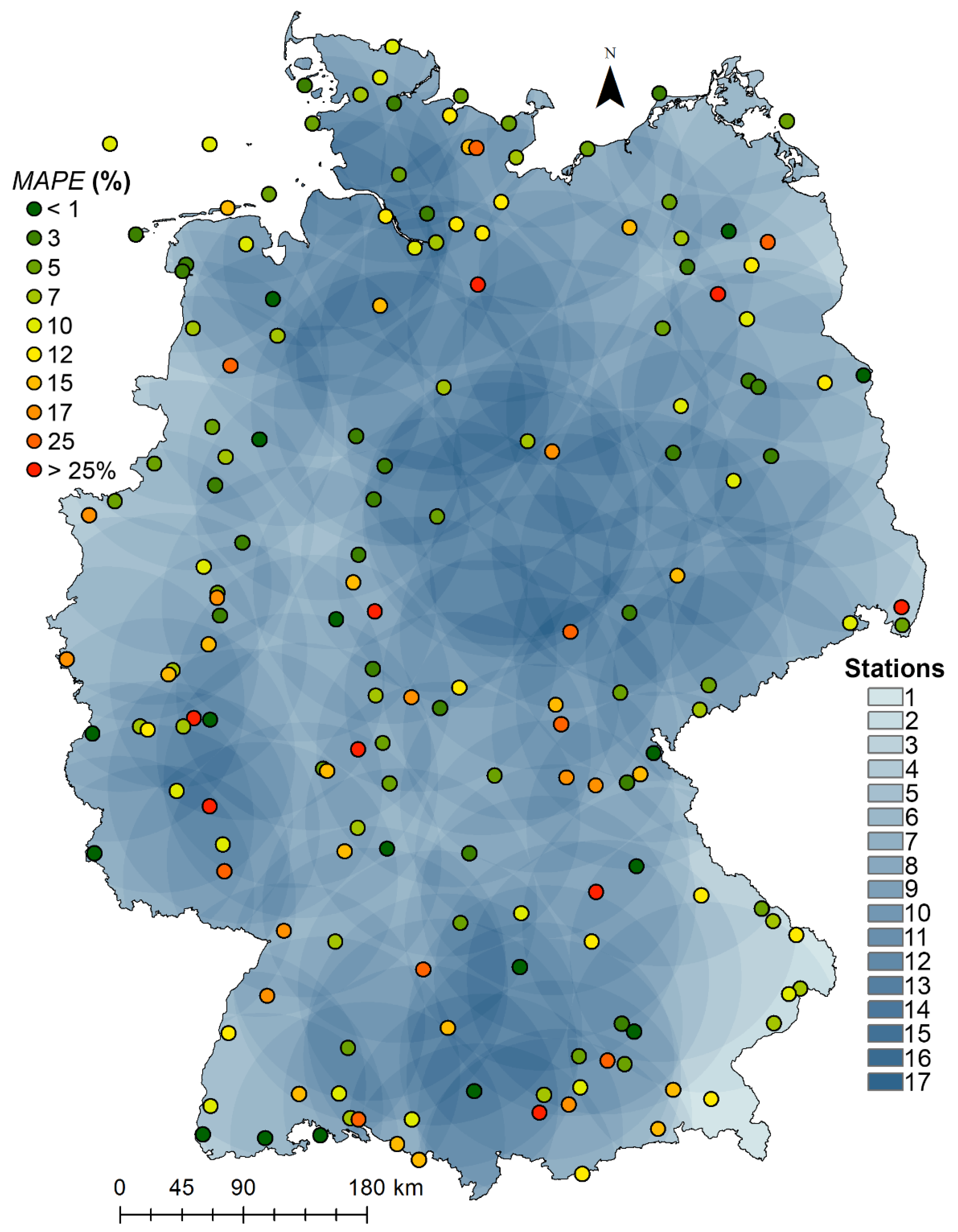
In general, it can be assumed that model accuracy is very high in areas with high measurement station density. To test if at a lower station density model accuracy decreases, the DS2 station-related mean absolute percentage error (MAPE) of GS over all storm events was calculated (Figure 10). MAPE is used here to compensate for the spatial differences in GS level in the study area. It was found that the median of all MAPE values is 7.34%. No clear spatial MAPE pattern occurs. Furthermore, no correlation between station density and MAPE was found, indicating that the model accuracy does not depend on the station density. It is therefore assumed that the GS model can be reliably applied throughout the study area.

4. Conclusions

In this study, it could be shown that on the basis of a large number of storms, it is possible to separate individual storm events from the median storm field over Germany. This enables both the probabilistic and spatially explicit quantification of the (1) storm hazard associated with the median gust speed field and (2) storm hazard associated with single catastrophic storm events. The results from the simulation clearly demonstrate that each storm event leads to unique gust speed fields.
It is obvious that the storm-specific gust speed fields show completely different characteristics in the study area. A good example of their variability is the comparison of storm Lothar with storm Kyrill. Due to the event-specific characteristics of their gust speed fields, the two storms led to significantly different damage patterns. The catastrophic damage caused by storm Lothar can be explained by the fact that its gust speed field intensity deviates most strongly from the median gust speed field in a narrowly defined area where many objects such as forests and buildings, which could not withstand the extreme wind loads connected with the gusts, occurred. This is also expressed by the unique shape of the survival function associated with storm Lothar.
The simulated gust speed fields now make it possible to explicitly assign the damage caused by individual storm events to a specific gust speed intensity. Due to the probabilistic modeling approach, one is no longer bound to the analysis of individual storm events, but can make spatially high-resolution statements about the storm hazard independent of storm events, which can ultimately lead to better risk management. Moreover, the probabilistic structure of the model enables the development of storm event scenarios under climate change in future studies.

Author Contributions

C.J. and D.S. developed the research idea, carried out data analysis and wrote the manuscript.

Funding

This work was supported by the Federal Ministry for the Environment, Nature Conservation and Nuclear Safety within the framework of the Forest Climate Fund (MiStriKli 28W-K-4-166-01).

Conflicts of Interest

The authors declare no conflict of interest.

References

  1. Munich RE NatCatSERVICE. Available online: https://natcatservice.munichre.com/ (accessed on 28 May 2019).
  2. Jung, C.; Schindler, D.; Buchholz, A.; Laible, J. Global Gust Climate Evaluation and Its Influence on Wind Turbines. Energies 2017, 10, 1474. [Google Scholar] [CrossRef]
  3. Hagen, M.; Bartenschlager, B.; Finke, U. Motion characteristics of thunderstorms in southern Germany. Meteorol. Appl. 1999, 6, 227–239. [Google Scholar] [CrossRef]
  4. Kunz, M. The skill of convective parameters and indices to predict isolated and severe thunderstorms. Nat. Hazards Earth Syst. Sci. 2007, 7, 327–342. [Google Scholar] [CrossRef] [Green Version]
  5. Kunz, M.; Sander, J.; Kottmeier, C.H. Recent trends of thunderstorm and hailstorm frequency and their relation to atmospheric characteristics in southwest Germany. Int. J. Climatol. 2009, 29, 2283–2297. [Google Scholar] [CrossRef] [Green Version]
  6. Pilorz, W.; Laskowski, I.; Łupikasza, E.; Taszarek, M. Wind Shear and the Strength of Severe Convective Phenomena—Preliminary Results from Poland in 2011–2015. Climate 2016, 4, 51. [Google Scholar] [CrossRef]
  7. Gregow, H.; Laaksonen, A.; Alper, M.E. Increasing large scale windstorm damage in Western, Central and Northern European forests, 1951–2010. Sci. Rep. 2017, 7, 46397. [Google Scholar] [CrossRef]
  8. Donat, M.G.; Leckebusch, G.C.; Pinto, J.G.; Ulbrich, U. Examination of wind storms over Central Europe with respect to circulation weather types and NAO phases. Int. J. Climatol. 2010, 30, 1289–1300. [Google Scholar] [CrossRef]
  9. Rasilla, D.; García-Codron, J.C.; Garmendia, C.; Herrera, S.; Rivas, V. Extreme Wave Storms and Atmospheric Variability at the Spanish Coast of the Bay of Biscay. Atmosphere 2018, 9, 316. [Google Scholar] [CrossRef]
  10. Basu, S.; Zhang, X.; Wang, Z. A Modeling Investigation of Northern Hemisphere Extratropical Cyclone Activity in Spring: The Linkage between Extreme Weather and Arctic Sea Ice Forcing. Climate 2019, 7, 25. [Google Scholar] [CrossRef]
  11. Durst, C.S. Wind speeds over short periods of time. Meteorol. Mag. 1960, 89, 181–186. [Google Scholar]
  12. Shanmuganathan, S.; Sallis, P. Data Mining Methods to Generate Severe Wind Gust Models. Atmosphere 2014, 5, 60–80. [Google Scholar] [CrossRef] [Green Version]
  13. Schelhaas, M.-J.; Nabuurs, G.-J.; Schuck, A. Natural disturbances in the European forests in the 19th and 20th centuries. Glob. Chang. Biol. 2003, 9, 1620–1633. [Google Scholar] [CrossRef]
  14. Schindler, D.; Grebhan, K.; Albrecht, A.; Schönborn, J.; Kohnle, U. GIS-based estimation of the winter storm damage probability in forests: A case study from Baden-Wuerttemberg (Southwest Germany). Int. J. Biometeorol. 2012, 56, 57–69. [Google Scholar] [CrossRef]
  15. Jung, C.; Schindler, D.; Albrecht, A.; Buchholz, A. The Role of Highly-Resolved Gust Speed in Simulations of Storm Damage in Forests at the Landscape Scale: A Case Study from Southwest Germany. Atmosphere 2016, 7, 7. [Google Scholar] [CrossRef]
  16. Valverde, L.J., Jr.; Convertino, M. Insurer Resilience in an Era of Climate Change and Extreme Weather: An Econometric Analysis. Climate 2019, 7, 55. [Google Scholar] [CrossRef]
  17. Hang, J.; Li, Y. Ventilation strategy and air change rates in idealized high-rise compact urban areas. Build. Environ. 2010, 45, 2754–2767. [Google Scholar] [CrossRef]
  18. Liu, L.; Wen, Y.; Liang, Y.; Zhang, F.; Yang, T. Extreme Weather Impacts on Inland Waterways Transport of Yangtze River. Atmosphere 2019, 10, 133. [Google Scholar] [CrossRef]
  19. Manasseh, R.; Middleton, J.H. The surface wind gust regime and aircraft operations at Sydney Airport. J. Wind Eng. Ind. Aerodyn. 1999, 79, 269–288. [Google Scholar] [CrossRef]
  20. Etienne, C.; Lehmann, A.; Goyette, S.; Lopez-Moreno, J.I.; Beniston, M. Spatial predictions of extreme wind speeds over Switzerland using generalized additive models. J. Appl. Meteorol. Climatol. 2010, 49, 1956–1970. [Google Scholar] [CrossRef]
  21. Augter, G.; Roos, M. Berechnung von Sturmintensitäten für Deutschland; Berichte des Deutschen Wetterdienstes; Deutscher Wetterdienst: Offenbach am Main, Germany, 2011; No. 236. (In German)
  22. Jung, C.; Schindler, D. Modelling monthly near-surface maximum daily gust speed distributions in Southwest Germany. Int. J. Climatol. 2016, 36, 4058–4070. [Google Scholar] [CrossRef]
  23. Schindler, D.; Jung, C.; Buchholz, A. Using highly resolved maximum gust speed as predictor for forest storm damage caused by the high-impact winter storm Lothar in Southwest Germany. Atmos. Sci. Lett. 2016, 17, 462–469. [Google Scholar] [CrossRef]
  24. Jung, C.; Schindler, D. Sensitivity analysis of the system of wind speed distributions. Energy Convers. Manag. 2018, 177, 376–384. [Google Scholar] [CrossRef]
  25. Jung, C. High Spatial Resolution Simulation of Annual Wind Energy Yield Using Near-Surface Wind Speed Time Series. Energies 2016, 9, 344. [Google Scholar] [CrossRef]
  26. Wan, H.; Wang, X.; Swail, V.R. Homogenization and trend analysis of Canadian near-surface wind speeds. J. Clim. 2010, 23, 1209–1225. [Google Scholar] [CrossRef]
  27. Walshaw, D. Getting the most from your extreme wind data: A step by step guide. J. Res. NIST 1994, 99, 399–411. [Google Scholar] [CrossRef]
  28. Wieringa, J. Does representative wind information exist? J. Wind Eng. Ind. Aerodyn. 1996, 65, 1–12. [Google Scholar] [CrossRef]
  29. Petersen, E.L.; Mortensen, N.G.; Landberg, L.; Højstrup, J.; Frank, H.P. Wind power meteorology. Part I: Climate and turbulence. Wind Energy 1998, 1, 25–45. [Google Scholar] [CrossRef]
  30. Jung, C.; Schindler, D. Development of a statistical bivariate wind speed-wind shear model (WSWS) to quantify the height-dependent wind resource. Energy Convers. Manag. 2017, 149, 303–317. [Google Scholar] [CrossRef]
  31. CORINE Land Cover. Available online: https://land.copernicus.eu/pan-european/corine-land-cover (accessed on 28 May 2019).
  32. CDC (Climate Data Center). Available online: https://cdc.dwd.de/portal/ (accessed on 28 May 2019).
  33. Wang, X.L. Accounting for autocorrelation in detecting mean-shifts in climate data series using the penalized maximal t or F test. J. Appl. Meteorol. Climatol. 2008, 47, 2423–2444. [Google Scholar] [CrossRef]
  34. Wang, X.L. Penalized maximal F-test for detecting undocumented mean shifts without trend-change. J. Atmos. Ocean. Technol. 2008, 25, 368–384. [Google Scholar] [CrossRef]
  35. EU DEM. Available online: https://land.copernicus.eu/imagery-in-situ/eu-dem (accessed on 28 May 2019).
  36. Wilson, J.D. Determining a topex score. Scott. For. 1984, 38, 251–256. [Google Scholar]
  37. European Settlement Map. Available online: https://land.copernicus.eu/pan-european/GHSL (accessed on 28 May 2019).
  38. Silva, J.; Ribeiro, C.; Guedes, R. Roughness length classification of Corine Land Cover classes. In Proceedings of the European Wind Energy Conference, Milan, Italy, 7–10 May 2007. [Google Scholar]
  39. Friedman, J. Greedy function approximation: A gradient boosting machine. Ann. Stat. 2001, 29, 1189–1232. [Google Scholar] [CrossRef]
  40. Van Heijst, D.; Potharst, R.; van Wezel, M. A support system for predicting eBay end prices. Decis. Support Syst. 2008, 44, 970–982. [Google Scholar] [CrossRef] [Green Version]
  41. Jung, C.; Schindler, D. 3D statistical mapping of Germany’s wind resource using WSWS. Energy Convers. Manag. 2018, 159, 96–108. [Google Scholar] [CrossRef]
  42. Wood, S.N. Thin-plate regression splines. J. R. Stat. Soc. Ser. B 2003, 65, 95–114. [Google Scholar] [CrossRef]
  43. Heneka, P.; Hofherr, T.; Ruck, B.; Kottmeier, C. Winter storm risk of residential structures—Model development and application to the German state of Baden-Württemberg. Nat. Hazards Earth Syst. Sci. 2006, 6, 721–733. [Google Scholar] [CrossRef]
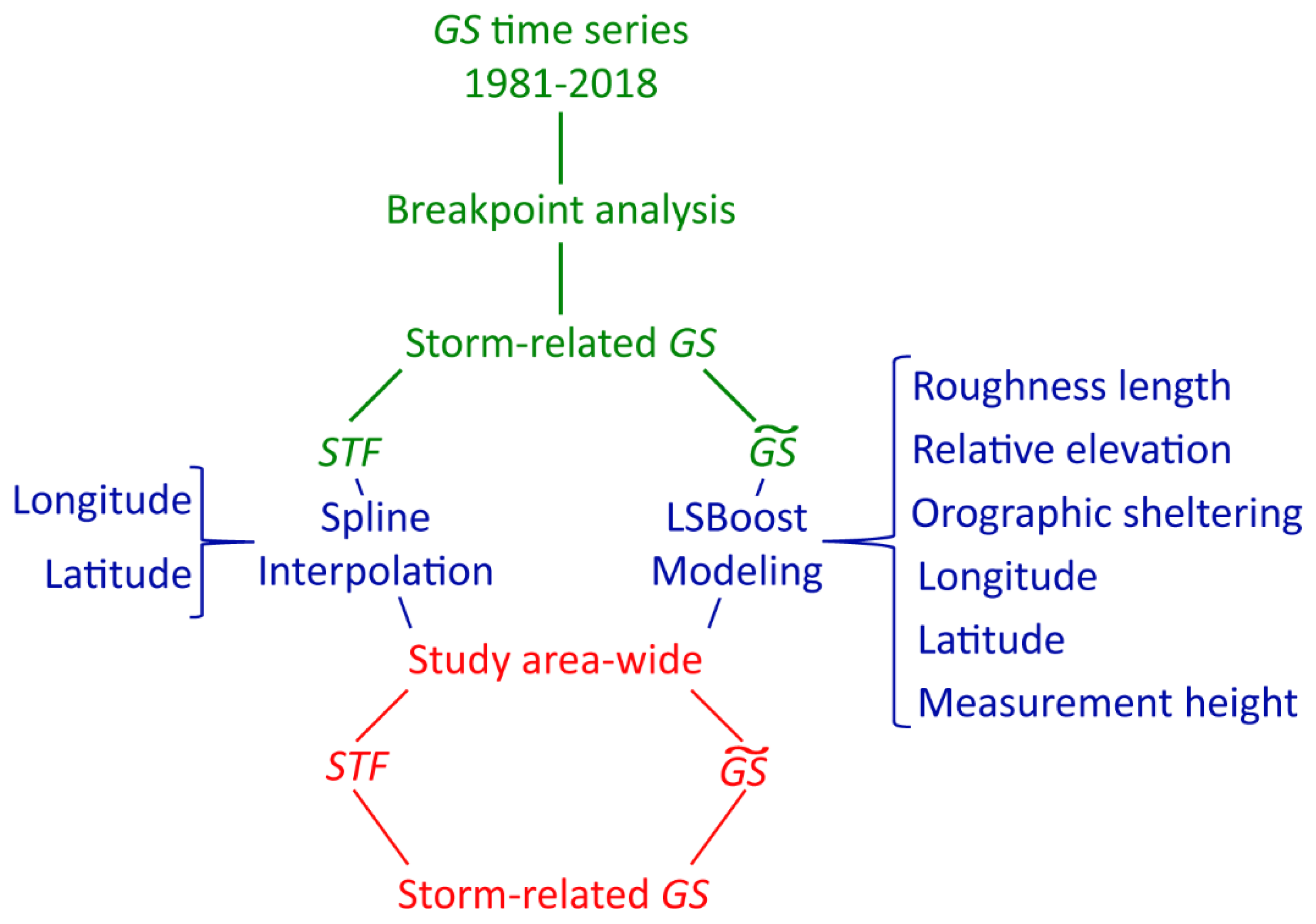
Figure 1. Overview of the methodology applied to develop Germany’s winter storm atlas (GeWiSA), with STF being the storm field factor, G S is the gust speed and G S ˜ is the median of G S .
Atmosphere 10 00387 g001
Figure 2. Gust speed (GS) measurement stations subdivided into a parameterization dataset (DS1) and test dataset (DS2).
Atmosphere 10 00387 g002
Figure 3. Median gust speed ( G S ˜ ) of all winter storms included in GeWiSA.
Atmosphere 10 00387 g003
Figure 4. Map extracts of median gust speed ( G S ˜ ) in the regions (a) north of the city of Frankfurt and (b) around the Brocken.
Atmosphere 10 00387 g004
Figure 5. Storm field factor (STF) of the winter storms (a) Daria; (b) Lothar; (c) Kyrill and (d) Friederike.
Atmosphere 10 00387 g005
Figure 6. Survival functions (SF) of the winter storm-related storm field factor (STF) representing the share of study area. The eight most severe winter storms are labeled with their ID. The two winter storms (ID: 77, Kyrill; ID: 51: Lothar) which caused the greatest losses are colored red. The six next severe winter storms are colored blue. The grey lines indicate all other winter storms.
Atmosphere 10 00387 g006
Figure 7. Gust speed (GS) fields of the winter storms (a) Daria; (b) Lothar; (c) Kyrill and (d) Friederike.
Atmosphere 10 00387 g007
Figure 8. Survival functions (SF) of the winter storm related gust speed (GS) representing the share of study area. The eight most severe winter storms are labeled with their ID. The two winter storms (ID: 77, Kyrill; ID: 51: Lothar) which caused the greatest losses are colored red. The six next severe winter storms are colored blue. The grey lines indicate all other winter storms.
Atmosphere 10 00387 g008
Figure 9. Storm event-related (a) coefficient of determination (R2) and (b) mean absolute error (MAE) of the parameterization dataset (DS1) and the test dataset (DS2). Please note the different scaling of the y-axes.
Atmosphere 10 00387 g009
Figure 10. Number of parameterization dataset (DS1) stations in a 100 km radius and mean absolute percentage error (MAPE) related to DS2 measurement stations.
Atmosphere 10 00387 g010
Table 1. Winter storms included in GeWiSA [1].
IDWinter StormDurationLosses
(US$m)
IDWinter StormDurationLosses
(US$m)
1-3 January 815150Winnie24–25 October 98130
2-3 February 812551Lothar26 December 992200
3-15–16 December 822652Anatol3–4 December 99410
4-9 October 821353Lara4–6 February 99140
5-10 December 82854Ginger28 May 00310
6-18 January 8313055Kerstin29–30 January 00120
7-26–28 November 8313056Oratia29–30 October 0093
8-1 February 8311057-10–11 December 0015
9-22–24 November 8422058-9 November 0131
10-3 January 845859Jeanett26–28 October 021700
11-20 October 842960Anna26–27 February 02730
12-7–8 February 84361Jennifer28–29 January 02410
13-6 December 854462Calvann2–3 January 03360
14-6 November 852963January21 December 03120
15-19–20 December 8643064Hanne12–14 January 04330
16-20–23 October8643065-17 December 04320
17-19–20 January8643066Oralie20–21 March 04270
18-12 November 87967Queenie31 January–1 February 04170
19-29 February–1 March 888668Gerda12–13 January 04140
20-7–8 October 882669Cyrus15–16 December 05530
21-8–9 October881770Thorsten25–27 November 05320
22-6 December 88971Erwin8–9 January 05160
23-19 December 88572Ulf12–13 February 05140
24-4–6 April 891873Ingo21 January 0574
25Daria25–26 January 90180074Britta31 October–2 November 06520
26Vivian25–27 February 90180075-30 December 06–1 January 07130
27Wiebke28 February–1 March 90180076Vera8 December 0667
28Herta3–4 February 9090077Kyrill18–19 January 075100
29Ottilie/Polly13–15 February 9027078Franz11–12 January 0793
30Nora17–18 October 913079Fridtijof2–3 December 0751
31Undine6–9 January 91780Emma1–2 March 08840
32Ismene26 November 9273081Kristen12 March 08250
33Coranna11–12 November 9228082Resi31 January–1 February 084
34-13 March 92783Annette23–24 February 083
35Wilma26 October 92484Quinten9–10 February 0953
36-2–3 December 92385Xynthia28 February 10920
37Verena13–14 January 9350086Joachim16–17 December 11200
38Barbara23–24 January 9324087Andrea5–6 January 12240
39Quena8–9 December 9320088Ulli/Emil3 January 1282
40Victoria19–21 December 9316089Christian27–29 October 13830
41Agnes22–23 January 9315090Xaver5–7 December 13260
42Lore27 January 9452091Niklas30 March–1 April 151200
43Grace4–5 November 95792Elon/Felix8–11 January 15260
44Sonja27–29 March 9726093Xavier5 October 17500
45Daniela19–20 February 9721094Herwart29 October 17290
46Gisela/Heidi25 February 9710095Sebastian13–14 September 17160
47-13–14 February 977896Egon12–13 January 17120
48Xylia27–29 October 9837097Friederike18 January 181900
49-4–5 March 9827098Burglind3 January 18240
Table 2. Predictor variables (PV) for modeling gust speed (GS) with DWD being the German Meteorological Service, EU-DEM is a digital elevation model and ESM is the European Settlement Map.
SymbolNameSector (°)Distance (m)Data SourceOriginal Resolution
hmeasuring height--DWD-
lonlongitude----
latlatitude----
εelevation --EU-DEM v.120 m × 20 m
η1000relative elevation1–3601000EU-DEM v.120 m × 20 m
η3000relative elevation1–3603000EU-DEM v.120 m × 20 m
η5000relative elevation1–3605000EU-DEM v.120 m × 20 m
η7500relative elevation1–3607500EU-DEM v.120 m × 20 m
ηnrelative elevation337.5–22.43000EU-DEM v.120 m × 20 m
ηnerelative elevation22.5–67.43000EU-DEM v.120 m × 20 m
ηerelative elevation67.5–112.43000EU-DEM v.120 m × 20 m
ηserelative elevation112.5–157.43000EU-DEM v.120 m × 20 m
ηsrelative elevation157.5–202.43000EU-DEM v.120 m × 20 m
ηswrelative elevation202.5–247.43000EU-DEM v.120 m × 20 m
ηwrelative elevation247.5–292.43000EU-DEM v.120 m × 20 m
ηnwrelative elevation292.5–337.43000EU-DEM v.120 m × 20 m
σnsheltering337.5–22.41000EU-DEM v.120 m × 20 m
σnesheltering22.5–67.41000EU-DEM v.120 m × 20 m
σesheltering67.5–112.41000EU-DEM v.120 m × 20 m
σsesheltering112.5–157.41000EU-DEM v.120 m × 20 m
σssheltering157.5–202.41000EU-DEM v.120 m × 20 m
σswsheltering202.5–247.41000EU-DEM v.120 m × 20 m
σwsheltering247.5–292.41000EU-DEM v.120 m × 20 m
σnwsheltering292.5–337.41000EU-DEM v.120 m × 20 m
σsumsheltering1–3601000EU-DEM v.120 m × 20 m
z0,25roughness length1–36025ESM 2012 R 20172.5 m × 2.5 m
z0,100roughness length1–360100ESM 2012 R 20172.5 m × 2.5 m
z0,200roughness length1–360200ESM 2012 R 20172.5 m × 2.5 m
z0,400roughness length1–360400ESM 2012 R 20172.5 m × 2.5 m
z0,nroughness length337.5–22.4400ESM 2012 R 20172.5 m × 2.5 m
z0,neroughness length22.5–67.4400ESM 2012 R 20172.5 m × 2.5 m
z0,eroughness length67.5–112.4400ESM 2012 R 20172.5 m × 2.5 m
z0,seroughness length112.5–157.4400ESM 2012 R 20172.5 m × 2.5 m
z0,sroughness length157.5–202.4400ESM 2012 R 20172.5 m × 2.5 m
z0,swroughness length202.5–247.4400ESM 2012 R 20172.5 m × 2.5 m
z0,wroughness length247.5–292.4400ESM 2012 R 20172.5 m × 2.5 m
z0,nwroughness length292.5–337.4400ESM 2012 R 20172.5 m × 2.5 m
Table 3. Roughness length (z0) assigned to the European Settlement Map (ESM) 2012 R 2017 [37] land use classes with acronyms for non-built up (NBU), built up (BU) and Normalized Difference Vegetation Index (NDVI).
Namez0 (mm)
BU Buildings1600
BU Area-Street Green NDVI100
BU Area-Green Urban Atlas500
BU Area-Green NDVI500
BU Area-Streets100
BU Area-Open Space1
NBU Area-Street Green NDVI100
NBU Area-Green NDVI750
NBU Area-Streets100
NBU Area-Open Space30
Railways100
Water1
Table 4. Predictor variable combinations (PVC) yielding the highest coefficients of determination in DS2 ( R D S 2 2 ).
PVC1234567
1lonlathη5000ηswσnez0,sw
2lonlathη7500ηsσsumz0,400
3lonlathη7500ηsσsz0,sw