Article

Results of Three Years of Ambient Air Monitoring Near a Petroleum Refinery in Richmond, California, USA

1
Chevron Energy Technology Company, Houston, TX 77002, USA
2
Chevron Energy Technology Company, San Ramon, CA 94583, USA
*
Author to whom correspondence should be addressed.
Atmosphere 2019, 10(7), 385; https://doi.org/10.3390/atmos10070385
Submission received: 10 June 2019 / Revised: 30 June 2019 / Accepted: 9 July 2019 / Published: 11 July 2019
(This article belongs to the Section Air Quality)

Abstract

:
Recent regulatory and legislative developments in the state of California (e.g., Assembly Bill (AB) 1647 and AB 617) will increase the extent of air quality monitoring in communities near petroleum refineries and at facility fencelines. This work reports results over a three-year period for currently-installed community and fenceline air quality monitoring for the Chevron refinery in Richmond, California, USA. This paper presents the most comprehensive air quality dataset that has been published to date for a community near a petroleum refinery, including concentration of different air toxics (e.g., benzene, toluene, xylenes, etc.) and criteria air pollutants (e.g., ozone (O3), sulfur dioxide (SO2), and particulate matter (PM)). Instrumental techniques such as ultra-violet differential absorption spectroscopy (UV-DOAS), laser-based spectroscopy and real-time gas chromatography (GC) were used in the community and fenceline monitors. From 2015 to 2017, measured concentrations at community monitors near the Richmond refinery were generally below California thresholds for acute and chronic health (only two exceedances were observed for 8-h average benzene concentrations during the three-year monitoring period). Although more detailed speciation for volatile organic compounds (VOCs) and fine particulate matter (PM2.5) would be needed to confirm certain source profile identities, preliminary application of source apportionment methods indicates the prevalence of typical urban emission profiles, such as from traffic, in the measured community data.

1. Introduction

Long-term continuous monitoring of air quality in locations near industrial facilities, including petroleum refineries, is generally scarce, and few studies on long-term pollutant concentrations have been published in the peer-reviewed literature to date [1,2].
Although multiple monitoring studies have been conducted near petroleum refineries, these studies were usually limited in temporal coverage, spanning periods from hours to a few months, with some exceptions including seasonal sampling over longer periods of time [3,4,5,6,7,8]. Previous work on air quality at refinery perimeters primarily focused on monitoring multiple volatile organic compounds (VOCs), with more limited emphasis on measurements of particulate matter (PM), trace gases, metals, and polycyclic aromatic hydrocarbons (PAHs) [2,3,6,7,8,9,10,11,12].
Passive VOC sampling followed by off-line gas chromatography separation using mass spectrometry or flame ionization detectors (GC-MS/GC-FID) has been the predominant analytical method employed in previous monitoring campaigns [13,14,15,16], while higher time resolution quantification using techniques such as proton-transfer-reaction-MS have been reported in recent works [8,17]. In addition to air quality monitoring near petroleum refineries, the chemistry and downwind dynamics of emission plumes from refining facilities and in-situ refinery process emissions have been analyzed [18,19,20,21].
Receptor models including principal component analysis (PCA) and positive matrix factorization (PMF) have been employed in multiple studies to determine the contribution of distinct emission sources to the VOC levels observed in industrial areas, including from petroleum refining operations [13,22,23,24,25,26]. These studies have reported traffic, industrial process emissions and solvent usage as the major emission sources that contribute to VOC concentrations at the monitoring locations. Some of these works have also identified that petroleum refinery processes contribute to the observed VOC levels. However, the wide variation in refinery emission source profiles creates challenges to compare this type of emission source between studies [13,22,23,24].
Results from previous work indicate that alkanes, alkenes and aromatic species are the predominant VOCs in areas near petroleum refineries and that propane, hexane, pentane, and toluene/benzene are the main aliphatic and aromatic compounds observed, respectively [6,13,14]. Despite general agreement on observations, such as light alkanes being the most abundant VOC species in refinery perimeter areas [2,27], studies have reached different conclusions regarding the impacts of refinery emissions on nearby ambient VOC enhancement. While some works have found elevated VOC concentrations when compared to background sites and urban locations [8,9,10,14,28,29], other studies conducted at different sites worldwide have reported no major impact from petroleum refineries emissions on neighboring VOC and PAH atmospheric levels [3,4,5,6,7]. While Na et al. [14] reported higher concentrations of PM and VOCs nearby petroleum refineries in South Korea when compared to a downtown location, Baltrenas et al. [4] and Kalabokas et al. [5] found similar or lower VOC levels in Lithuania and Greece refinery neighboring areas when compared to urban centers in those countries. Gariazzo et al. [9] observed larger concentrations of alkanes, but no evident enhancement in aromatic VOCs nearby a refinery in Italy (when compared to a downtown location), while Wallace et al. [8] concluded that refinery operations were the driver of the levels of aromatic VOCs measured at a location near a refining facility in the Ship Channel area in Houston, Texas (USA).
Although specific meteorological conditions (i.e., wind direction and speed) impact the conclusions derived from these works, the temporal coverage of the measurements in these studies might be also insufficient to assess long-term concentration trends and differentiate potential confounding sources impacting air quality in locations near petroleum refineries, leading to these seemingly contrary results. Thus, more comprehensive air quality datasets are needed to better evaluate air quality dynamics and emission source impacts in this type of location.
Regulations in the state of California, such as AB 617 [30], are expected to increase ambient air quality monitoring in many locations throughout the state, including near some petroleum refineries, as part of a statewide effort to better inform air quality conditions and implement data-driven reduction initiatives of criteria pollutant and air toxic emissions in selected communities. Other regulations in the state will also require the installation of continuous monitors, including open-path, for multiple species of air pollutants along sections of refinery fencelines throughout the State [31].
A 2019 report by the California Environmental Protection Agency Office of Environmental Health Hazard Assessment (OEHHA) [32] provided a list of chemicals emitted from California refineries prioritized by estimated emissions levels and toxicity. The report lists these chemicals as the top candidates for air monitoring: acetaldehyde, ammonia (NH3), benzene, 1,3-butadiene, cadmium, diethanolamine, formaldehyde, hydrogen fluoride, hydrogen sulfide (H2S), manganese, naphthalene, nickel, nitrogen oxide, PAHs, PM, SO2, sulfuric acid, and toluene. The scope of the OEHHA report [32] did not include measurements to assess exposure or health risk in communities.
A subset of the compounds listed above, along with other species of interest, have been continuously measured at three fencelines and three community monitors near the Chevron refinery in Richmond, CA (USA) since 2013. The purpose of this work is to present long-term air pollution concentration results from the most recent three years (2015–2017) of fenceline and community-based monitoring data near this refinery. Analysis of a multi-location, multi-species, long-term concentration dataset near a petroleum refinery has not been presented in the peer-reviewed literature to date and, thus, this work constitutes a novel, comprehensive effort to evaluate air quality trends nearby a petroleum refining facility. Preliminary PMF and PCA were applied to identify the main sources contributing to the VOC levels observed at the three community monitoring sites and, when appropriate, based on the quality of the collected data, comparisons were made to regulatory health risk thresholds to contextualize the results from the measurements.

2. Materials and Methods

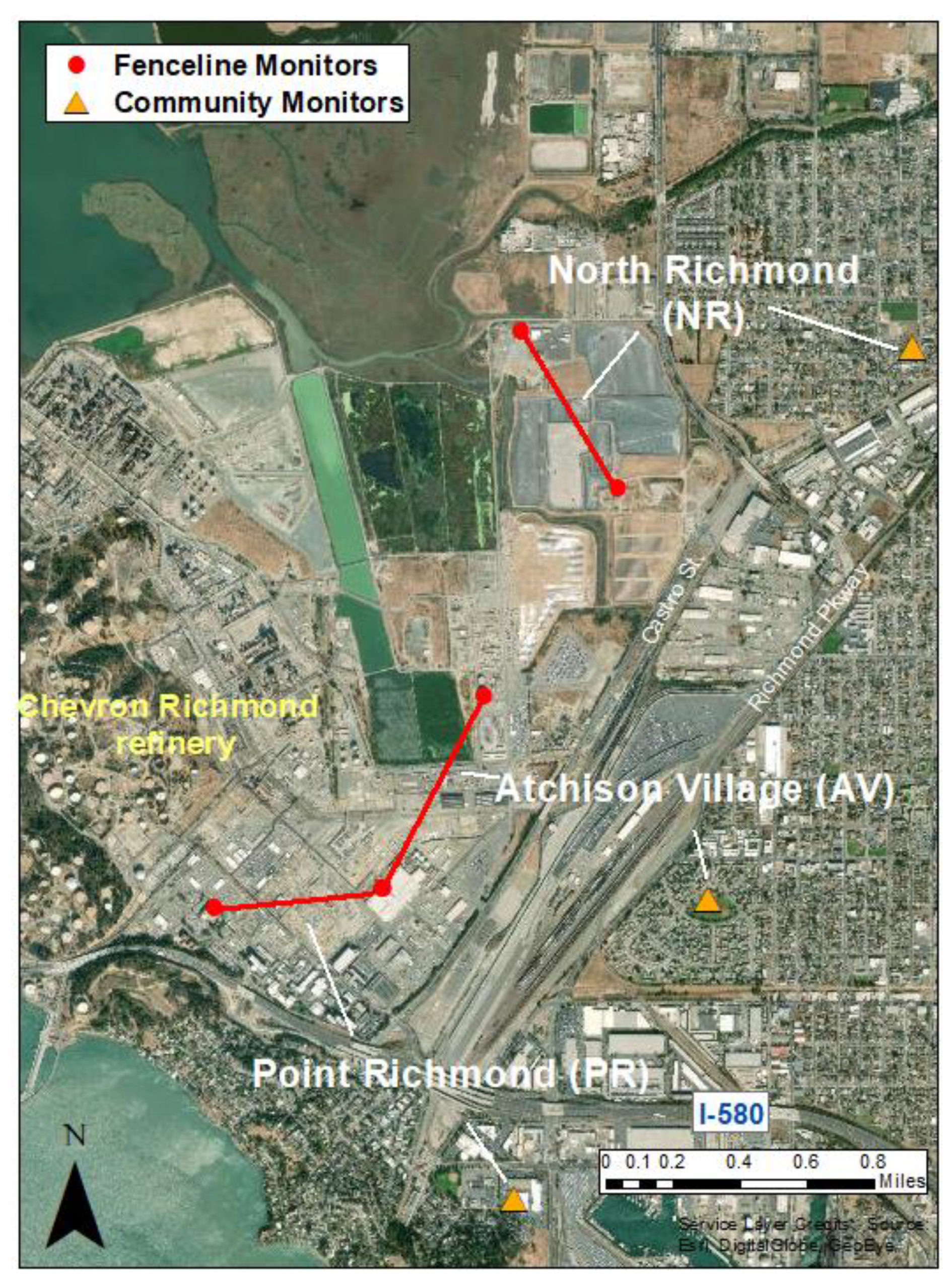
2.1. Description of Monitoring Network

The ambient air quality monitoring network near Richmond refinery consists of three open-path monitors along the refinery fenceline and three point-monitoring stations in the nearby community (referred to as community monitors in this manuscript) (Figure 1), that have been in operation since 2013 [33]. The three community monitoring locations—Atchison Village (AV), North Richmond (NR), and Point Richmond (PR)—are named for the neighborhood where the community monitor is located, and each community monitoring location has a like-named fenceline monitor along the refinery fenceline between the community monitoring location and process areas within the refinery. The monitoring network is operated and maintained by a third-party consultant, Argos Scientific, which was selected based on input from the City of Richmond, the refinery, and the local community [33]. Real-time and the most recent 24-h of measurement data for all species are available on a publicly-accessible website [34]. This work focuses on data collected from the monitoring network during the most recent three years between 2015 and 2017. A three-year period was chosen to align with timeframes for National Ambient Air Quality Standard (NAAQS) averaging in USA [35].
While additional continuous monitors, including open path, will be added to the refinery fenceline monitoring network by 2020 to comply with a new regulation (Regulation 12, Rule 15) from the Bay Area Air Quality Management District (BAAQMD) [36], the fenceline monitoring system that was operational during the study period included two open-path instruments at each monitoring location: an UV-DOAS manufactured by Argos Scientific (Camas, WA, USA) to measure several air toxics (carbon disulfide (CS2) benzene, toluene, and xylenes) and criteria pollutants (SO2 and O3) and a tunable diode laser (TDL) from Boreal Laser (Edmonton, AB, Canada) to measure H2S. Open-path monitors provide an average concentration measurement over the entire path-length between an analyzer and its retro-reflector, and path lengths in the fenceline monitoring network vary between 698 and 915 m. Each community monitoring location includes a Teledyne T201 analyzer for NH3 (Englewood, CO), a MetOne BAM 1020 for fine PM (PM2.5) (Grants Pass, OR, USA), a Teledyne API Model 633 analyzer for black carbon (BC), a Teledyne model T101 analyzer for H2S, and a Synspec, Inc. GC (Groningen, NL, USA) that measures a variety of air toxics and O3 precursor compounds (VOCs). Calibration and maintenance of these instruments is performed by Argos Scientific, including monthly GC calibration employing certified standard VOC mixtures purchased from Linde Gas (Bridgewater, NJ, USA) Technologies. The compounds to be detected at the monitoring sites were selected after consultation with a stakeholder group that included community groups, the local air district, and the City of Richmond [33]. More information on the compounds measured and instrument detection limits is available in Table S1 in the Supplementary Materials.
The community monitoring locations were selected based on input from the City of Richmond and from community meetings [33], as well as considerations for available site power, equipment security, and the absence of major point sources between the monitoring location and the refinery. As shown in Figure 1, there is a major highway and railyard located between the Point Richmond community monitor and the refinery, and high-traffic streets between the refinery and other two monitoring locations. It should also be noted that the monitoring network locations are not in the predominant downwind direction of the refinery since the wind generally blows from the refinery towards the unpopulated San Pablo Bay, and the monitoring network was designed to measure air pollutant concentrations in populated areas of communities where the wind blows in a 22.5° wind vector quadrant at least 10% of the time [33]. Between 2015 and 2017, the refinery was in the downwind direction of the Point Richmond, Atchison, and North Richmond community monitors approximately 90%, 85% and 80%, respectively, as shown in Figure S1.
This study primarily focused on the community monitoring locations because these instruments had lower detection limits than the fenceline monitoring locations, as shown in Table S1, and generated more above detection limit data. It should be noted that these community and fenceline monitoring networks were designed to provide rapid information to the nearby community on air quality concentrations (on a five-minute basis), and instrumentation was selected and operated to meet that objective. For these instruments, as it is for nearly all air pollutant measurement instruments, there are trade-offs between analytical cycle time and instrument detection limits (i.e., higher frequency analysis results in reduced sensitivity). Although the primary purpose of the monitoring system was not long-term ambient air assessment, the community monitoring dataset was found to provide novel insights into near refinery air quality.

2.2. Selection of Ambient Air Risk Screening Levels

Risk-based screening levels are derived from equations combining exposure assumptions with chemical-specific toxicity values. The exposure thresholds discussed throughout this manuscript were based on the acute, 8-h and chronic reference exposure levels (RELs) set by the California OEHHA [37] (Table S2). OEHHA determines RELs associated with human systems or organs (e.g., respiratory system) that could be affected by the noncancer effects of airborne chemicals. A detailed description of these reference levels and the rationale behind selections is included in the Supplementary Materials.

2.3. Source Apportionment Methodologies

2.3.1. Positive Matrix Factorization

PMF analysis of VOC concentrations at AV, NR and PR sites was conducted using speciated GC measurements to gain insight on the potential sources contributing to the measured levels of these species at each community monitor. PMF analysis was not conducted for PM as the PM2.5 measurement technique in the community monitors only provided overall concentration information, not composition, which is typical for most ambient air monitoring locations. PMF is a receptor model that outputs a profile of the contributing sources (factor profile) and their associated concentration (factor contribution to the observed concentrations of specific species). PMF analysis incorporates the experimental errors associated with the analytical quantification of VOCs and involves the minimization of a function Q (summation of squared scaled residuals) using a weighted linear least squares approach while incorporating non-negativity constraints [38]. In this study, EPA PMF 5.0 (USA EPA) was used to perform PMF analysis on the 1-h average AV, PR and NR VOC concentration datasets for each location. The experimental errors for each species (above and below the instrumental detection limit of 0.5 ppb) were calculated following the approach described by Polissar et al. [39]. The analytical uncertainty of the detection method was calculated using different calibration datasets (2015–2017) according to the procedure outlined in [40]. PMF models including two to six factors were evaluated for each dataset and the number of factors to be retained in each PMF model was defined based on the criteria described in the Supplementary Materials.

2.3.2. Principal Component Analysis

PCA was applied subsequently to PMF analysis to aid the PMF factor identification and classification. The PCA datasets included BC, NH3, H2S, PM2.5, concentrations of the PMF factors in the models selected at each community monitoring site, and meteorological variables (wind speed/direction, temperature and relative humidity-RH). PCA was performed on the correlation matrices of the 1-h average AV, PR and NR sites concentration datasets independently for each monitoring location using the package Psych for R (R version 3.2.5). Periods with missing data for any of the species were removed prior to PCA application. The adequacy of each dataset for PCA application was determined based on the Kaiser–Mayer–Olkin index and the Bartlett’s test of sphericity criteria (PCA Section in the Supplementary Materials). Following the Kaiser–Guttman criterion, principal components (PC) with eigenvalues > 1 were retained in each model, and the identity of each PC was established based on variables with loadings > 0.6 (at least ~40% of the variance of the variable is being explained by the corresponding factor) [8,41] (Supplementary Materials). The PC scores were calculated using the regression method described by Thurstone [42], and the diurnal trends of these scores for specific PCs were examined and used to support PC/PMF factor identification.

3. Results and Discussions

3.1. Ambient Air Monitoring Results

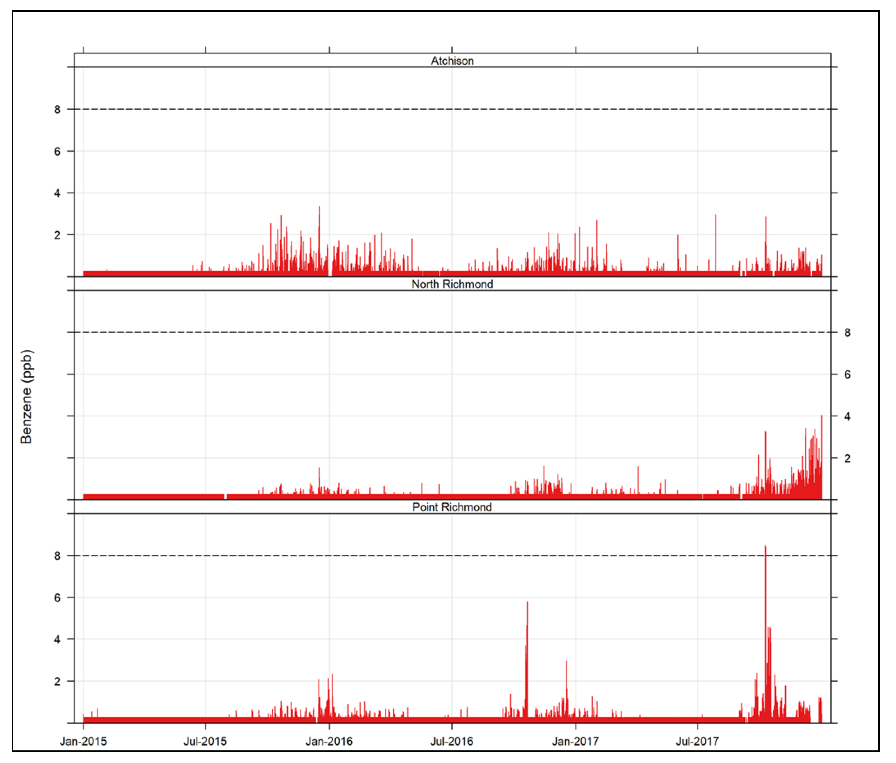
3.1.1. Community Data Overview

Table S3 shows the summary of data recovery at the three community monitoring stations from January 2015 to December 2017 for each of the seventeen species being quantified. Data recovery spanned a minimum of 93% (corresponding to a 7% PM2.5 missing data at AV) and maximum of 99.8% (corresponding to a 0.2% H2S missing data at the PR site). These data recovery levels are typical of air monitoring networks quantifying species such as VOCs and exceed data quality requirements established by EPA NAAQS monitoring stations [43,44]. Periods of missing data corresponded to instrument calibration intervals and times when instrumental and communication issues prevented data acquisition. Wind roses for periods of missing data for the different species at each monitoring site showed that winds were not particularly associated to the refinery direction during these intervals (winds blowing from the refinery less than 20% of the time at all monitoring locations, Figure S1). Detailed information on specific causes of missing data at the AV, PR and NR sites is presented in Table S4. BC had the highest percentage of detectable levels among the measured species, with no more than 5% non-detected values at each location. PM2.5 levels were lower than the detection limit of the instrument (6 µg/m³) for 36%, 33% and 37% of the measurements at the AV, NR and PR sites, respectively. NH3 levels at the community monitors were detected at moderate frequency (7%, 19% and 44% non-detected at AV, NR and PR sites, respectively). Organic compounds measured by the GC at the community locations included benzene, toluene, ethylbenzene, xylene (measured as both o-xylene and m,p-xylene isomers), n-heptane, n-hexane, n-octane, trimethylbenzene (measured as three different isomers), 3-methylpentane (3-MP) and 2,2,4-trimethylpentane (224-TMP). These organic compounds had a large fraction of non-detected values (up to 98% for some cases). The large number of non-detects observed for VOCs is consistent with the type of instrumentation operating in the community monitors, as discussed in Section 2.1. Below detection limit measurements were replaced with half of the instrument detection limit (shown in Table S1) across the dataset as recommended by Polissar et al. and Helsel [39,45]. Detailed discussion about spatial and temporal trends and comparisons for individual measured compounds is provided in the following sections.

3.1.2. Fenceline Data Overview

Table S5 shows the summary of data recovery at the three fenceline open-path monitors. As discussed in Section 2.1, pollutants measured at each fenceline pathlength included benzene, toluene, xylene, CS2, SO2 and O3 using a UV-DOAS system, and H2S using a TDL system. The detection limits of the instruments (Table S1) were generally higher than the typical ambient levels of these pollutants, except for O3. Therefore, it is not surprising that most of measurements were below detection limits: >98% non-detects for benzene, toluene, xylene, CS2 and H2S and >80% non-detects for SO2 across fenceline monitoring locations. As discussed in Section 2.1, the instruments located at the refinery fenceline were selected with community and City of Richmond input and based on the need for high time resolution concentration data (five-minute basis) for community informational purposes. The maximum hourly O3 values during 2015–2017 at the PR, NR and AV monitors were 69, 57 and 62 ppb, respectively, which were all below the O3 NAAQS (70 ppb, fourth-highest daily maximum, averaged across three consecutive years) [35]. Subsequent discussions in this manuscript focus on the community monitoring data considering that fenceline monitoring information that is relevant to average ambient conditions is limited.

3.1.3. Volatile Organic Compounds (VOC)

Table 1 shows the year-by-year annual average of benzene, toluene, ethylbenzene and xylenes (hereafter BTEX) at the three community monitoring stations. BTEX annual average values were all below the OEHHA chronic RELs, which were selected as screening levels (Table 1 and Table S2). The 1-h and 8-h RELs for benzene are 8 ppb and 0.93 ppb, respectively. For comparison, the 1-h and 8-h average benzene time series are presented in Figure 2 and Figure S2, respectively. The 8-h average concentrations for benzene exceeded the REL in a few instances over the 3-year study period as shown in Figure S2. One of such periods (October 2017) was coincident with the Northern California wildfire [46], which resulted in significant deterioration of air quality across the region. Similarly, the 1-h average concentrations of benzene, which were predominantly below the corresponding REL at all community locations (Figure 2), exhibited two exceedances at the PR site during this period (9 October 2017 and 10 October 2017). This is consistent with previous reports on benzene emissions from biomass burning and wildfires at different locations [47,48]. Similar increases in other combustion-related air pollutants such as PM2.5 and BC were also observed during this period, as discussed in Section 3.1.5. Benzene 8-h concentrations exceeded the REL between 15 October 2016 and 21 October 2016 at the PR monitor. Pollution roses constructed for this period (Figure S2) indicate that the benzene detected during this interval originates predominantly from the southwesterly direction (note that the refinery is located northwest of the PR site).
The 1-h average concentrations of toluene and xylenes measured at the community locations are shown in Figures S3 and S4. Concentration of these species were below the detection limit of the GC system (i.e., <0.5 ppb, replaced by 0.25 ppb in the dataset and figures) for most of the study period. The hourly average of the detected values for toluene and xylenes were well below the acute REL values; the maximum 1-h value for the three-year period was 51 ppb for toluene compared to a REL of 9800 ppb and 62 ppb xylenes as compared with a REL of 5000 ppb. Similarly, ambient levels of ethylbenzene, shown in Figure S5, were mostly below detection limit (>96% below 0.5 ppb) at all three community locations, and the maximum 1-h concentration measured was 6 ppb. It should be noted that there is no OEHHA acute REL available for ethylbenzene.
Several other VOCs, including n-hexane, n-heptane, n-octane, 3-MP and trimethylbenzenes (measured as three isomers, namely 1,2,3-trimethylbenzene (123-TMB), 1,2,4-trimethylbenzene (124-TMB), and 1,3,5-trimethylbenzene (135-TMB) were also measured at the community locations. As discussed in Section 3.1.1, these compounds were largely below instrumental detection limit at all three community monitors, and the few measured concentrations between 2015 and 2017 were all below the available chronic and acute RELs. The 1-h concentration of these compounds are presented in Figures S6 and S7.
Table S6 compares annual average BTEX concentrations measured at the three Richmond community monitoring stations with those measured at the six Contra Costa county BAAQMD stations reporting these species during 2015–2017 [49]. The location of these BAAQMD monitoring sites is presented in Figure S8. It is worth noting that direct comparison between VOC concentrations at the community monitors and the BAAQMD sites is limited due to differences in the sampling frequency and analytical methods used for detection. As discussed previously, the community monitors perform continuous 5-min GC-FID analysis with a detection limit of 0.5 ppb for BTEX, and one-half the detection limit was substituted for all non-detects in the analysis, so the minimum value reported here is 0.25 ppb. The BAAQMD sites collect 24-h VOC concentrations on a one-in-twelve-day sampling schedule (1/12), which results in approximately 30 reported measurements per year per site [50,51]. Additionally, the analysis of VOCs collected at the BAAQMD stations is conducted using GC-MS, a technique with a lower detection limit (0.12–0.16 ppb [52]) than GC-FID (0.5 ppb). Based on these considerations, Table S6 is presented here only for informative purposes.

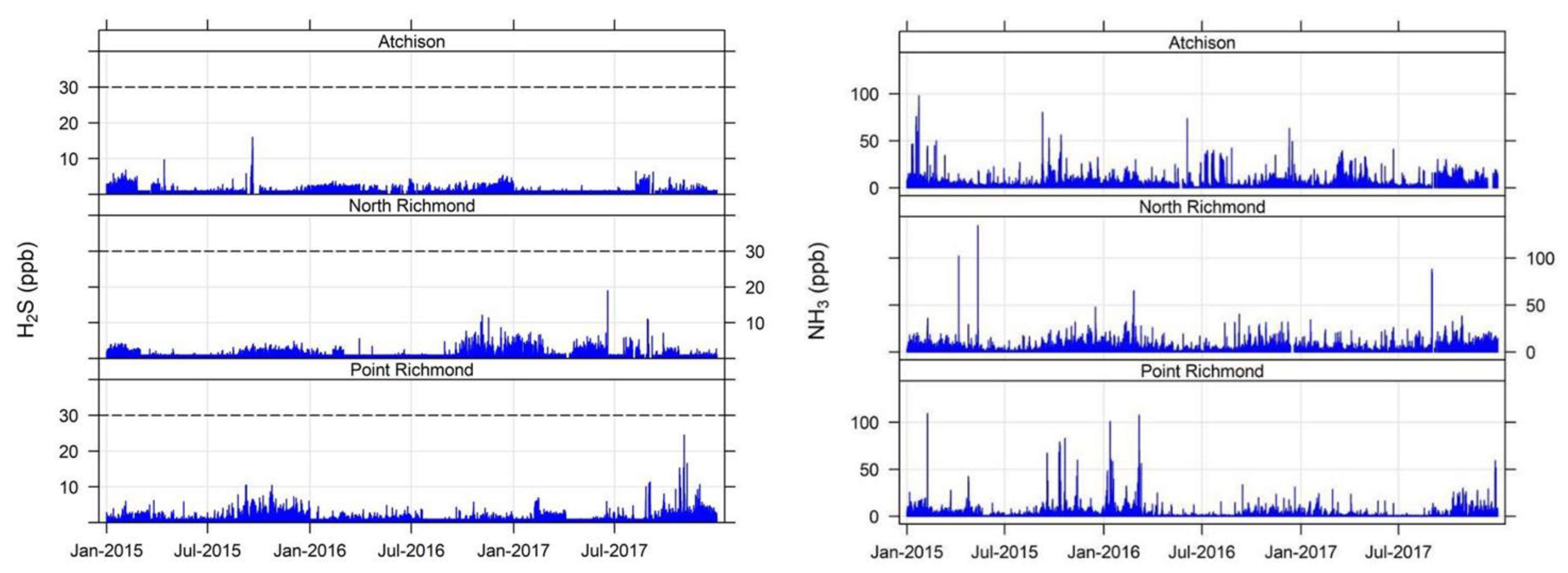
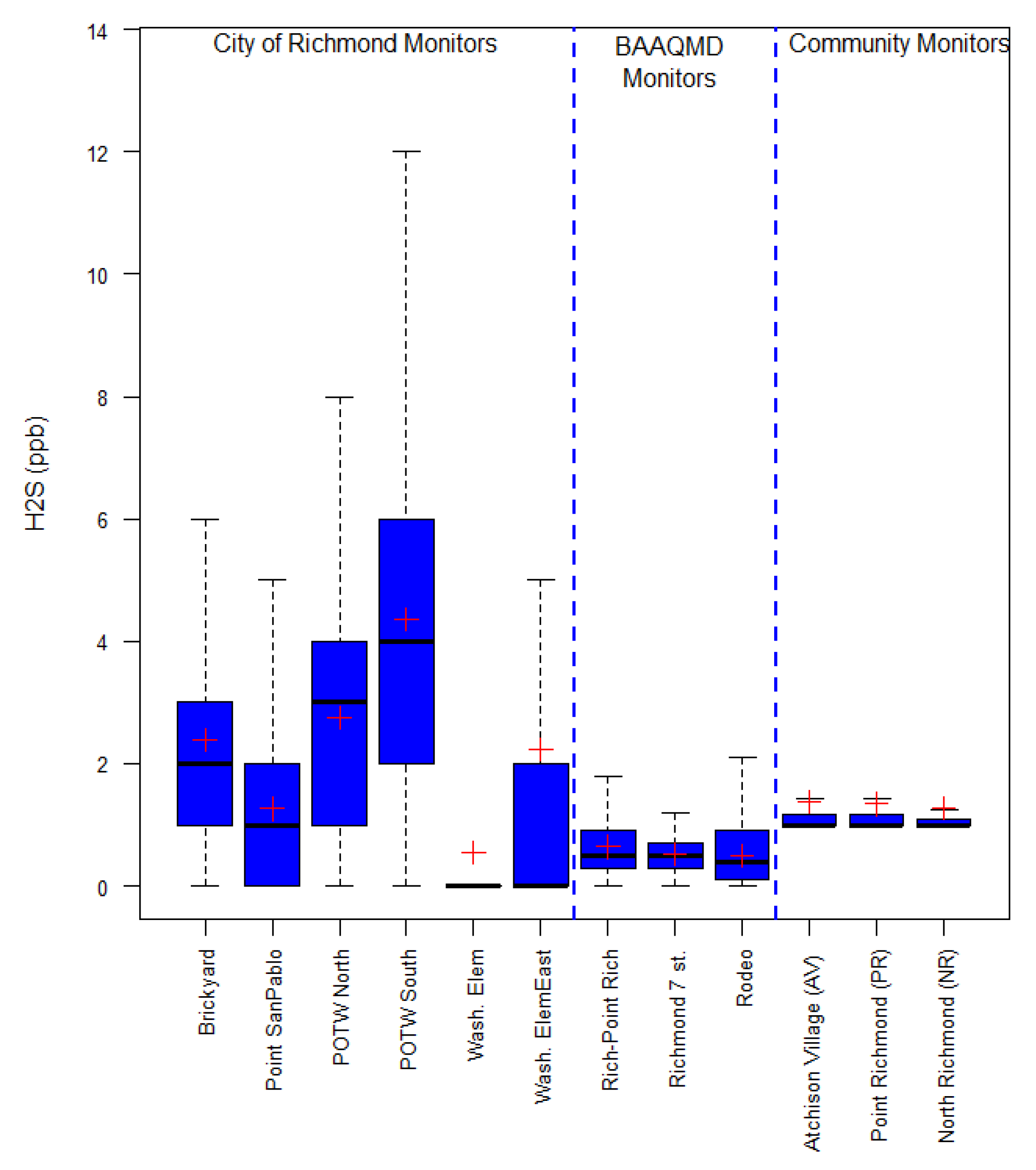
3.1.4. Hydrogen Sulfide and Ammonia

Annual average concentrations of hydrogen sulfide and ammonia were below the OEHHA chronic RELs for all years and locations, as shown in Table 2. Similarly, the 1-h concentrations of these gases were lower than the acute RELs, as depicted in Figure 3. Average annual concentrations of H2S and NH3 at the community monitors ranged between 1.1 and 1.6 and 2.6 and 6.3 ppb, respectively. Both species demonstrated significant temporal variability, with higher weekday compared to weekend concentrations and bimodal diurnal trends with a morning peak (potentially associated with the morning traffic rush hour period [53,54]) and a nighttime peak (likely attributable to stable atmospheric conditions and lower mixing height), as shown in Figure S9.
The concentrations of H2S observed at AV, NR and PR sites in 2015–2017 were compared with levels of this species detected at the three BAAQMD monitoring sites reporting H2S in Contra Costa county [49], as well as with concentrations reported by six City of Richmond monitors situated near the PR community monitor [55]. The location of these monitoring sites is presented in Figure S10.
Figure 4 presents the variation in the 1-h H2S concentrations at the BAAQMD, City of Richmond and community monitoring sites during 2015–2017. One-way analysis of variance (ANOVA-R 3.2.5 statistical package) indicated that average H2S concentration at the AV, NR and PR sites were significantly lower (p < 0.01) than at the City of Richmond monitoring sites and slightly larger than the levels detected at the BAAQMD stations. However, it is worth noting that direct inter-site comparison of H2S concentrations is limited due to the relatively high detection limit of the monitors employed at the community sites (2 ppb, Table S1). The distribution of concentrations presented in Figure 4 indicates that for the 2015–2017 period, H2S levels at the different monitoring sites (BAAQMD, City of Richmond, and community monitors) were primarily below the 1-h California Ambient Air Quality Standards (CAAQS) for this species (30 ppb) [56]. Differing variability in H2S concentrations was observed amongst monitoring sites, with relatively narrow ranges at AV/NR/PR sites and BAAQMD locations, and larger variability at the City of Richmond monitors (first and third inter-quartile variation up to 4 ppb). The three City of Richmond monitors with the highest average and median H2S concentrations (Figure 4) were furthest in distance from the refinery (Figure S10) and located near a wastewater treatment plant.

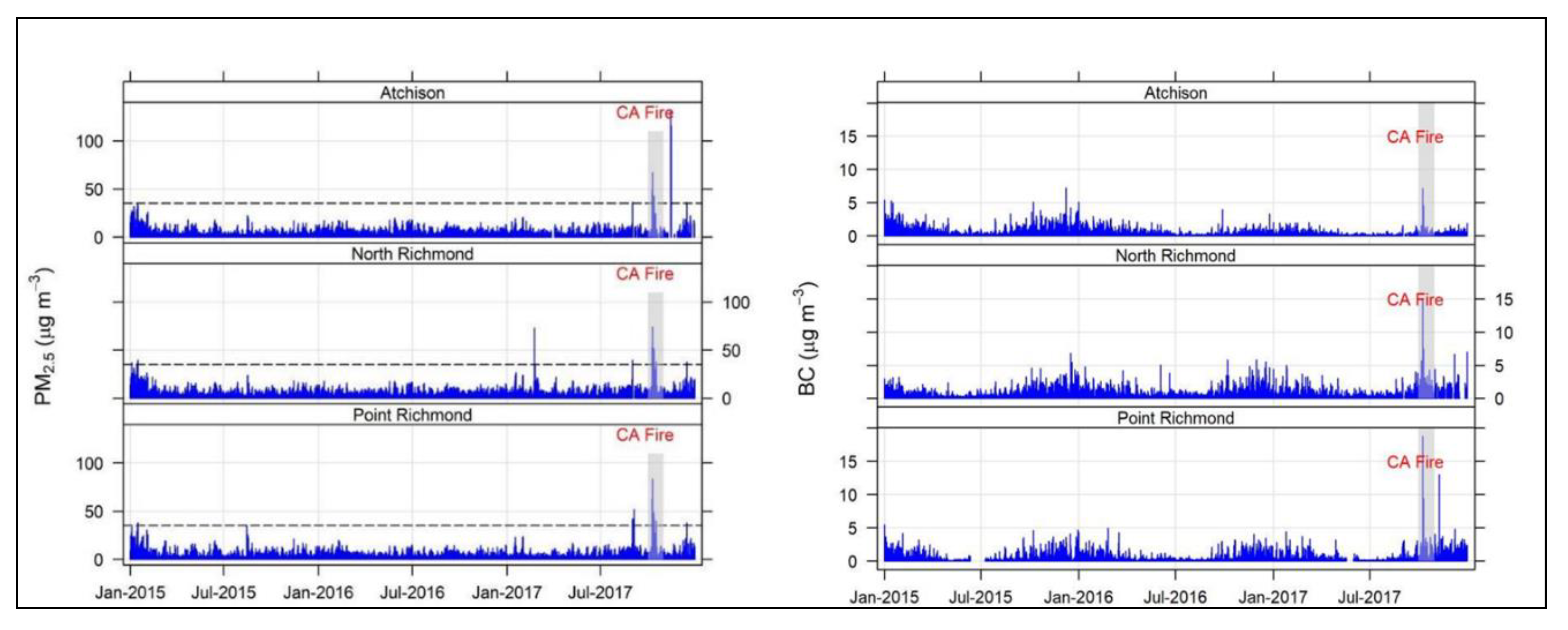
3.1.5. PM2.5 and Black Carbon

Concentration time series as well as annual average concentrations of particulate pollutants measured at the community monitoring stations, including PM2.5 and BC are shown in Figure 5 and Table 2, respectively. For PM2.5, there is no chronic or acute REL value set by the California OEHHA, but PM2.5 is a criteria air pollutant and is therefore regulated by the USA EPA through implementation of NAAQS. As shown in Figure 5, 24-h average PM2.5 concentrations were generally below the 24-h NAAQS threshold of 35 µg/m3, except for a period in October 2017 that was coincident with the Northern California wildfire [46]. A similar peak was observed for BC concentrations during that period (as well as for benzene, as discussed in Section 3.1.3). Annual average BC concentrations ranged between 0.25 and 0.53 µg/m3 across the study period and sites as shown in Table 2, which were within the same range or lower than other urban areas in California. For comparison, the average annual BC concentration of 1.3 µg/m3 was reported for cities in the South Coast air basin in the recent Multiple Air Toxics Exposure Study conducted by the local air quality management district [57]. Moreover, the annual average concentration of PM2.5 (ranging between 7 and 10 µg/m3 across monitoring sites) was below the relevant chronic thresholds (i.e., three-year CAAQS and NAAQS standards of 12 µg/m3), as shown in Table 2. As with NH3 and H2S (discussed in the previous section), PM2.5 and BC also had significant temporal variability, with higher concentration during the colder months of the year (December–February) attributable to lower atmospheric mixing height, as well as higher weekday compared to weekend concentrations and bimodal diurnal trends with a morning peak (associated with the morning traffic rush hour period) and a nighttime peak (likely attributable to stable atmospheric conditions and lower mixing height) [58,59], as shown in Figure S11.
The levels of PM2.5 at the community monitors during 2015–2017 were compared with the concentrations observed in the three BAAQMD monitoring sites reporting PM2.5 in Contra Costa county (Figure S12). Figure 6 presents box plots of PM2.5 concentration at each monitoring site. Comparable PM2.5 levels were observed at the distinct locations, with no evident enhancements in concentrations observed at the sites nearby the refinery. One-way ANOVA indicated that PM2.5 average 1-h concentrations at the AV and PR sites were significantly lower than the levels at the three BAAQMD monitoring sites [49], while concentrations at the NR site were significantly lower than those observed at San Pablo and Concord BAAQMD sites (p < 0.01). As presented in Figure S13, the 24-h NAAQS exceedances observed in the community monitors in late 2017 during the Northern California wildfire [46] were also evident in the three PM2.5 BAAQMD monitors located in other parts of Contra Costa County. In addition to the site-wide 24-h NAAQS exceedances, a period of increased concentration was noticed exclusively at the NR monitor during February 2017 (Figure 5 and Figure S13). This period was further investigated using conditional bivariate probability function (CBPF) plots [60] (OpenAir package for R, (R 3.2.5)) to establish the wind directional dependence of the elevated PM2.5 concentrations (Figure S14). According to Figure S14, the highest probability of concentrations above the 95th percentile during this period (66 ug/m3) was related to high speed winds blowing from the northeast, although no specific source type was evident (the refinery is located west to southwest of the NR site).

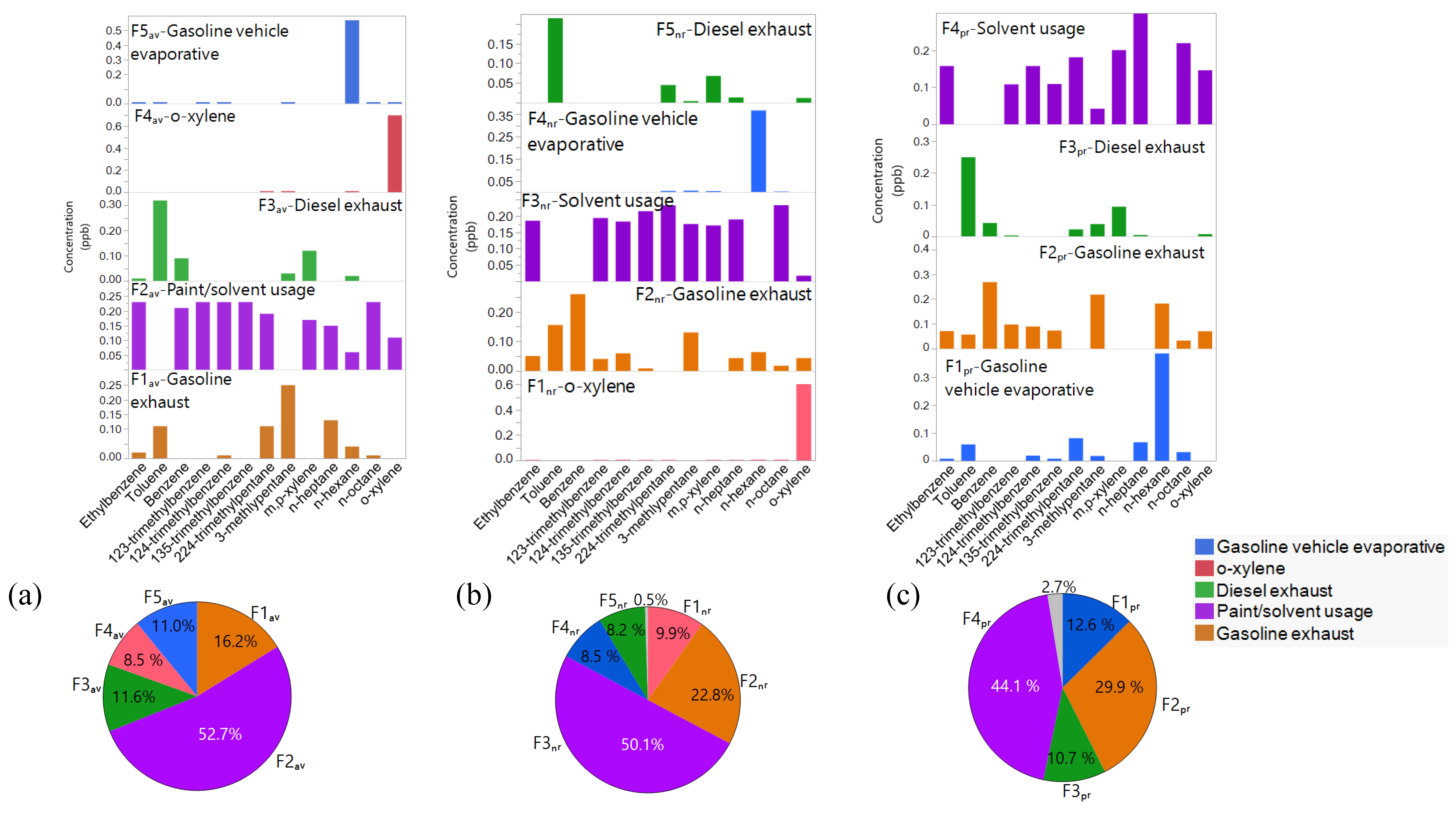
3.2. VOC Source Apportionment

PMF analysis of the different VOC datasets and subsequent application of the evaluation criteria described in Section 2.3 led to the selection of five-factor (AV and NR sites) and four-factor (PR site) models for the community monitoring sites. Further information on PMF and the factor selection process is presented in the Supplementary Materials (Figures S15–S20). After establishing the number of PMF factors to be retained at each community location, PCA was independently performed on the AV, NR and PR sites datasets to aid factor identification (as described in Section 2.3). Discussion on the classification and identification of the PMF factors at each community monitor is presented in the following sections.

3.2.1. Atchison Village

The factor profiles of the five PMF factors retained at the AV site are illustrated in Figure 7 and Figure S21. As presented in Figure 7, Factor 1 at the AV site (F1AV), which contributes to an average 16.2% of the VOC concentrations at this location, exhibits high contributions from 3-MP, 224-TMP, toluene, n-heptane and n-hexane. Species such as 3-MP and 224-TMP have been reported as tracers of gasoline vehicular emissions at different urban locations and 3-MP has been proposed as an exclusive indicator of vehicular activity [61,62,63]. According to the SPECIATE 4.5 database [64], n-hexane is typically present in gasoline exhaust, while generally absent in diesel exhaust emissions source profiles.
Additionally, toluene and n-heptane have been reported in gasoline tailpipe emissions in different studies worldwide [61,65,66,67,68]. The diurnal profile of F1AV, presented in Figure S22, indicates an increase in this factor during the morning traffic rush hour and some peak increases in concentration during daytime, with a secondary peak around 21:00 PT, indicating a potential link between F1AV and gasoline exhaust emissions [58,59]. Although benzene would be expected in a factor reflecting gasoline vehicle emissions, some previous studies have also reported gasoline tailpipe factors with negligible presence of this species [62,69].
Toluene, benzene, m,p-xylene and 3-MP are the predominant species in Factor 3 at the AV site (F3AV), which constitutes 11.6% of the average VOC concentrations at this community monitor. The diurnal profile of F3AV, presented in Figure S22, resembles the typical behavior of tracers of vehicular emissions (e.g., BC and PM), with marked peaks in the morning and evening traffic rush hours [58,59]. The species present in F3AV have been widely reported as traffic markers [24,70], and F3AV closely agrees with the concentration source profile reported by Yuan et al. [71] for diesel vehicles.
Factor 5 at the AV site (F5AV) (11% of average VOC concentration at this site, Figure 7) exhibited high contributions from n-hexane, with minor contributions from n-octane, o-xylene and 3-MP among others. n-hexane is a typical species in gasoline vehicle evaporative source profiles [64,72] and large vehicular emissions of this species have been reported in urban locations [73,74]. The diurnal trends of F3AV (Figure S22) concur with previous gasoline evaporation emission profiles reported in the literature [24] and indicate increased concentrations during the afternoon, consistent with increased evaporation rates at higher ambient temperatures.
PCA application on the AV site dataset led to the retention of five factors, explaining over 60% of the variance of the dataset (PCs with eigenvalues > 1) (Table S7). Loadings of F1AV–F5AV > 0.6 were observed mainly in the first PC (PC1AV) (17.5% of the explained variance (EV)) (Table S8), indicating that PC1AV was able to capture over 40% of the variation observed for these variables. The high loadings of BC in PC1AV and the concurrence of F1AV, F3AV and F5AV in this factor indicates an association between these variables. Considering (i) the diurnal profile of PC1AV (Figure S23); (ii) the fact that BC is a typical marker of vehicular emissions [8,75]; (iii) the abundance of specific traffic-related species in F1AV, F3AV and F5AV; and (iv) the diurnal trends of F1AV, F3AV, and F5AV, these factors are classified in this study as gasoline exhaust, diesel exhaust and gasoline vehicle evaporative, respectively.
Factor 2 at the AV site (F2AV) exhibits a more complex source profile than the other PMF factors identified at this location and contributes to 52.7% of the average VOC concentrations at this monitoring site. The large complexity of F2AV factor profile, as well as the abundance of aromatic species including m,p-xylene, o-xylene, ethylbenzene, 123-TMB, 124-TMB and 135-TMB, are consistent with a solvent usage factor [69,76,77]. F2AV also comprises large concentrations of heptane, n-octane and benzene, which are reported in different solvent-related factor profiles included in the SPECIATE 4.5 database [64]. Furthermore, F2AV exhibits similarities with solvent-based paint, auto painting, architectural coatings and surface coating factor profiles reported previously at different locations [24,69,78]. The diurnal profile of F2AV (Figure S22), which shows concentration increases during daytime, is consistent with increased evaporation rates expected at higher temperatures. PC5AV in Table S8 shows high loadings of F2AV concurrent with moderate loadings of PM2.5, indicating association between this factor and aerosols concentrations. Although reports have identified solvent utilization as a major contributor to secondary organic aerosols (SOA) formation [79], additional information on the character of PM2.5 at the AV site would be necessary to establish a potential link between F2AV and SOA. Based on this information, F2AV is classified here as related to composite paint and solvent usage. Further discussion on the categorization of this factor is presented in Section 3.2.4.
Factor 4 at AV (F4AV), which represents 8.5% of the average concentrations of VOCs at this location, is primarily constituted by o-xylene. PC3AV (Table S8) shows moderate loadings of this factor along with NH3 concentrations. Although o-xylene and NH3 have been associated with emissions from mobile sources [24,53], the diurnal profile of F4AV is not consistent with traffic patterns. Additionally, F4AV is not related with tracers of vehicular emissions such as BC. The CBPF plot of F4AV (Figure S24) shows increased probabilities of concentrations (~8%) associated to intermediate speed (~2–5 m/s) southeasterly winds, indicating that F2AV is likely linked to an unidentified o-xylene emission source located at the southeast of the AV monitoring site (recall that the Chevron refinery is located west/southwest from the AV site, as illustrated in Figure 1). Based on the available information, complete identification of F2AV is not possible and, thus, it is categorized here as an o-xylene emission source.

3.2.2. North Richmond

Figure 7 and Figure S25 present the PMF factor profiles and the average contributions of the identified factors to the VOC concentrations at the NR community monitor.
Factors 2,4 and 5 at the NR site (F2NR, F4NR and F5NR), which contribute to 22.9, 8.5 and 8.2% of the VOC average concentration at this site, respectively, exhibited high influence from vehicular activity markers, as illustrated in Figure 7. Specifically, F2NR resembles previously reported gasoline exhaust factor profiles, with the presence of particular gasoline tailpipe tracers such as 3-MP, hexane, heptane and 1,2,4-TMB [63,64,74]. Although the predominance of benzene over toluene in F2NR is not usually observed in mobile gasoline combustion sources, gasoline exhaust profiles with similar characteristics have been reported previously [26]. As discussed for the AV site, the diurnal behavior of F2NR (Figure S26) resembles typical hourly traffic patterns, reinforcing the association of this factor with vehicular activity.
The diurnal profile of F4NR (Figure S26) agrees with that of F5AV (Figure S22) and exhibits large contributions from n-hexane, which, as discussed in the case of the AV site, is consistent with gasoline vehicle evaporation sources.
F5NR exhibits a similar diurnal profile than F2NR (Figure 7), indicating the association of this factor with traffic emissions. Species predominant in F5NR, such as toluene, 2,2,4-TMP and m,p-xylene, are well known markers of vehicles emissions [24,67]. The absence of n-hexane and n-heptane in this factor suggests that F5NR could correspond to diesel vehicle emissions, as these species are usually more abundant in gasoline tailpipe emissions [64]. The lack of benzene in F5NR has been previously reported for diesel exhaust emissions factors [26]. Furthermore, the lower concentrations of aromatic VOCs in F5NR when compared to F2NR point out to contributions from diesel vehicle combustion [62].
As in the case of the AV site, PCA was applied to the NR site dataset. Five PCs, explaining over 60% of the variance in the dataset, were retained in the model (Table S7). PCA factor loadings are presented in Table S9. As for the AV site, loadings above 0.6 for F1NR–F5NR were only observed in the first PC (PC1NR ~ 22% EV), which shows concurrence between F2NR/F4NR/F5NR and BC, a tracer of traffic activity. This result, along with the diurnal profile of PC1NR (Figure S27), further support the classification of F2NR, F4NR and F5NR as gasoline exhaust, gasoline vehicle evaporative emissions, and diesel vehicle emissions, respectively.
Factor 1 at the NR site (F1NR), which exhibits almost exclusive concentrations of o-xylene and contributes to almost 10% of the VOC concentrations at this location, showed peak levels at 18:00 PT (Figure S26). PCA did not provide specific insight on the origin of F1NR, and its CBPF plot (Figure S28) indicated that as in the case of F4AV, increased probabilities of concentration exceeding the 95th percentile for this factor were associated with intermediate speed (~4 m/s) southeasterly winds. Thus, based on the available information, F1NR is categorized as a factor related to the unidentified o-xylene emission source observed at the AV monitoring site.
Factor 3 at NR (F3NR) exhibits a complex profile with presence of diverse VOC species and contributes to over 50% of the VOC levels at this location. As in the case of F2AV, species typically related to solvent usage (m,p-xylene, 1,2,3-TMB, 1,2,4-TMB, 1,3,5-TMB and ethylbenzene) are present in this factor. Simultaneous occurrence of trisubstituted benzenes has been previously observed in auto painting and coatings source profiles [24,69], reinforcing the potential association between F3NR and solvent utilization sources. F3NR exhibits similarities to the concentration profiles of industrial coatings and a silk-screen cleaning solvent reported in previous studies [67,80], although it is worth noting that toluene and benzene (absent from F3NR) were also observed in the silk-screen solvent emission profile reported by Tang et al. [80]. F3NR shows elevated concentrations during the daytime, consistent with higher evaporation rates at higher ambient temperatures. Based on this discussion, F3NR is classified here as an aggregated factor related to solvent usage. Further discussion on the categorization of F3NR is presented in Section 3.2.4.

3.2.3. Point Richmond

The source profile of the four factors retained in the PMF model at the PR site are presented in Figure 7 and Figure S29, with the respective factor contributions to the VOC concentrations at this location summarized in Figure 7.
PCA application at the PR site led to the retention of 4 PCs (aggregated EV of ~56%) at this monitoring site (Table S7). Large loadings of PMF Factors 1–3 (F1PR, F2PR, and F3PR), BC and PM2.5 were observed in the first PC at PR (PC1PR-EV ~23%) (Table S10), indicating the association of these PMF factors with traffic emissions (as discussed for the AV and PR sites). The diurnal profile of PC1PR, presented in Figure S30, further supports this observation. The presence of PM2.5 in PC1 (concurrent with BC) suggests that PM at this location might have a more primary origin [8] than at AV, where PM2.5 exhibited large loadings concurrent with solvent usage factor concentrations.
The diurnal behavior (Figure S31) and the concentration profile of F1PR (Figure 7), which exhibits predominant concentrations of n-hexane, agree with F5AV and F1NR. Based on the discussion presented in previous sections, this factor, contributing to ~13% of the VOC levels at the PR site, was classified as gasoline vehicle evaporative emissions.
Similarly, F2PR and F3PR, contributing to ~30 and 11% of the VOC levels at the PR site, respectively, were classified as gasoline and diesel exhaust emissions, correspondingly. As shown in Figure 7, these factors exhibit large contributions from mobile source exhaust tracers, including 3-MP, hexane, toluene, benzene and 2,2,4-TMP [63,64,74]. The diurnal profiles of these factors confirm their association with vehicle traffic activity and resemble the hourly trends of the traffic-related factors in the AV and PR sites (Figures S22, S26 and S31). The larger influence of aromatic VOCs and n-hexane observed in F2PR when compared to F3PR suggests that F2PR and F3PR correspond to gasoline and diesel exhaust emissions, respectively [62].
PMF Factor 4 at the PR site (F4PR) exhibits a complex concentration source profile consistent with the solvent usage factor identified at the NR site, although with larger levels of n-heptane. This species is predominant in several solvent usage factor profiles, including paint thinning solvents and degreasing composite factor reported previously [64,80] and thus, F4PR (contributing to ~44% the VOC concentrations at the PR site) is accordingly classified here as a composite solvent usage factor. As in the case of the AV and NR sites, additional discussion on this solvent usage factor is presented in Section 3.2.4.

3.2.4. Inter-site Comparison of VOC source Contributions

As summarized in Table 3, factors identified as paint/solvent usage (F2AV, F3NR and F4PR), constituted the major contributor to the observed VOC levels at the three monitoring sites. As discussed in Section 3.2.1, Section 3.2.2 and Section 3.2.3, the factor profiles of F2AV, F3NR and F4PR were consistent with solvent usage factors reported in the literature. Despite this consistency, prior to final categorization of these factors as related to solvent usage, different potential sources, including refinery and industrial emissions were considered. Comparison between F2AV, F3NR and F4PR concentration profiles and refinery/petrochemical sources profiles reported in the literature [13,23,24,76] indicated important differences in both type and species contributions. C1–C4 alkanes and alkenes are predominant in the refinery/petrochemical source profiles, and although these species were not measured at the community monitors, other species relevant in refinery profiles such as benzene, toluene and n-hexane [13,23,24,76] were generally absent from the factors categorized as solvent usage, except in the AV site, where benzene and a minor contribution of n-hexane were observed (Figure 7). Similarly, VOCs with high contributions to F2AV, F3NR and F4PR (e.g., ethylbenzene, n-octane, n-heptane, 123, 124 and 135-TMB) are not usually predominant in refinery emission profiles [13,23,24,76]. It should be noted that species such as 124-TMB, present in F2AV, F3NR and F4PR, have been associated to the C9 aromatic fraction from petroleum refining and although not typical, specific studies have reported 123, 124 and 135-TMB as relevant in refinery/petroleum products emission profiles [22,81]. To further investigate potential association between F2AV, F3NR and F4PR and refinery emissions, pollution wind roses were generated for these factors (Figure S33). As illustrated in Figure S33, no substantial association was observed between F2AV/F3NR/F4PR concentrations and winds from the refinery direction, reinforcing the discussion in Section 3.2.1, Section 3.2.2 and Section 3.2.3 and supporting the categorization of these factors as related to solvent usage.
The contributions to the VOC levels at the AV and NR community monitors followed the sequence solvent usage > traffic activity > o-xylene emission source. The o-xylene factor, which encompasses the total concentrations of this species at the AV and NR sites (Figures S21 and S25), was not observed at the PR site. At this location, o-xylene levels were mainly distributed between solvent usage and gasoline exhaust emissions, as illustrated in Figure S29.
The solvent usage factors explained on average between 44.1% and 52.7% of the VOC concentrations at the three community monitors, with the largest contribution observed at AV. The contribution related to solvent use was followed by average traffic apportionments (gasoline/diesel exhaust and gasoline vehicle evaporative) ranging between ~39% and 53%. Similar influence from traffic activity was noticed at the AV and NR sites (close to 40% of VOC concentrations), while increased impact of this source was observed at the PR site, where traffic-related emissions contributed to over 53% of the observed VOC levels. At this site, gasoline exhaust and gasoline vehicle evaporative were the largest contributors among the traffic-related sources and exceeded the impact of these emission sources at the AV and NR sites. In the case of diesel vehicles exhaust emissions, comparable contributions were observed at the PR and AV sites (~11% of VOC levels), while slightly lower VOC concentrations (~8%) were apportioned to this factor at the NR site. The predominance of traffic activity at the PR site is consistent with the proximity of this location to major roads such as the I-580, located north of the PR monitoring site (Figure 1). The influence of emissions from vehicles on the I-580 on the VOC levels at PR is evidenced by the CBPF plots of the traffic-related factors at this site (F1PR, F2PR and F3PR), which are presented in Figure S32.
The paint/solvent usage factor at the AV, NR and PR sites explained most of the concentration of 9–10 of the 13 VOC species quantified at these sites, as illustrated in Figures S21, S25 and S29. Common VOC species were observed in the concentration profile of the solvent usage factor at the distinct monitoring sites (Figure 7), including ethylbenzene, n-heptane, m,p-xylene, 224-TMP and 123, 124 and 135-TMB. The concentration profiles of this factor exhibited similar characteristics at the AV and NR sites, where comparable species distributions were observed. Larger differences where noticed between the AV/NR and PR sites solvent usage factors, with a less homogeneous profile including larger contributions of n-heptane observed at the PR site.
The traffic-related factors encompassed most of toluene, benzene, 3-MP and n-hexane concentrations at the monitoring sites, except for AV, where approximately 30% of the benzene concentration was associated with vehicular emission factors. As discussed previously, low concentrations or absence of benzene in traffic emission factors have been previously reported [26,76]. Additionally, benzene has been apportioned to emission sources other than vehicular activity even at locations where large traffic influence is observed [8].
In addition to the solvent usage and traffic-related factors, an o-xylene emission source contributed to approximately 8–10% of the VOC concentrations at the AV and NR sites (F4AV and F1NR, respectively). As discussed in the previous sections, complete identification of this emission source was not possible based on the available information, although CBPF plots indicated that higher concentrations of this factor were associated with intermediate speed southeasterly winds. Interestingly, an o-xylene factor also appeared when PCA analysis was performed on the concentrations datasets (BC, NH3, PM2.5, H2S, VOC concentrations and temperature/RH) at these locations (results not presented).
Although the source apportionment conducted in this study is valuable to better understand potential VOC contributors at the community monitoring locations, it should be noted that annual average VOC concentrations across monitoring sites were below available OEHHA chronic RELs (Section 3.1.1), and therefore, PMF analysis here had a primarily explorative purpose.

4. Conclusions

This study examined three years of air pollution concentration data from three community-based air quality monitoring stations in Richmond, California, USA. The community monitors are in the neighborhoods near a petroleum refinery but are not situated in the predominant downwind direction from the refinery (there are no neighborhoods immediately situated in the predominant downwind direction). This study represents the first time that such an extensive community monitoring dataset near a refinery has been published in the peer-reviewed literature. For the sites in this study, concentrations of speciated VOCs, H2S, NH3, PM2.5, and BC were generally below established acute and chronic regulatory thresholds.
Comparison with BAAQMD air quality monitors located in Contra Costa county indicated that the concentrations of PM2.5 at the community monitors were statistically lower than at District monitoring sites in other parts of the same county. Direct comparison of H2S and VOC levels was limited due to differing analytical techniques and associated detection limits between the Richmond community sites and the BAAQMD monitors.
Source apportionment based on PMF analysis complemented with PCA application indicated that the air quality at the monitoring sites had relevant influence from traffic sources and solvent usage. As identification of VOC source profiles is challenging due to the wide variation of reports in the literature for specific emission sources (e.g., solvent usage), additional data would be needed to inform more detailed source apportionment exercises. These data could include speciated PM2.5 sampling and extended VOC speciation profiles that would likely need a different GC technology than the one used in this study, which was installed to provide rapid air quality information to the local community and not specifically designed for source apportionment studies. If additional PMF analyses were desired, the extended VOC detection capabilities should target markers of particular emission sources that allow more precise identification of these sources (e.g., C1–C4 alkanes and alkenes for refinery emissions, acetylene and isopentane for gasoline exhaust and gasoline vehicle evaporative emissions, respectively), which would be beyond the original intent of the community monitoring network. However, since measured concentrations of VOC at the existing community monitoring network were below OEHHA chronic RELs for the compounds of interest, such a detailed data gathering effort may not be a priority for future work. Despite the limitations of the collected datasets for source apportionment exercises, certain types of sources such as vehicular emissions were discernable from the air species concentrations quantified in this study.
The different analyses presented in this paper for the 2015–2017 period suggest that concentrations of the measured air species at the community monitoring sites located in Richmond, CA were comparable to other locations in Contra Costa county and that, based on the observations from the monitoring sites included in this study, the refinery operations were not likely to be the dominant driver of elevated air pollutant concentrations in the Richmond communities where the monitoring sites are located.

Supplementary Materials

The following are available online at https://www.mdpi.com/2073-4433/10/7/385/s1, Table S1: List of species, analyzers, and detection limits for each of the three community and fenceline monitoring locations in the network near the Richmond Refinery, Table S2: OEHHA acute, 8-h and chronic REL values corresponding to the species measured at the Richmond fenceline and community monitoring networks. Table S3: Summary of the air quality measurements at the community monitoring stations, including percent missing data and percent non-detected values, Table S4: Percentage of missing data associated to calibration periods and instrumental issues at the community monitoring sites during 2015–2017. Table S5: Summary of the air quality measurements at the fenceline, including percent missing data and percent non-detected values at each pathway, Table S6: Annual 24-h average benzene, toluene, ethylbenzene and m,p-xylene concentrations at the community monitors and at six BAAQMD monitoring sites in Contra Costa county, Table S7: PCA results for Atchison Village, North Richmond and Point Richmond monitoring sites, Table S8: Variable loadings for principal components with eigenvalues above 1 resulting from PCA application on the Atchison Village dataset, Table S9: Variable loadings for principal components with eigenvalues above 1 resulting from PCA application on the North Richmond dataset, Table S10: Variable loadings for principal components with eigenvalues above 1 resulting from PCA application on the Point Richmond dataset, Figure S1: Wind rose plots for each community monitoring location in the monitoring network for 2015–2017, Figure S2: Benzene 8-h average concentration (ppb) at the three community monitoring stations, including Point Richmond, North Richmond and Atchison. Figure S3: Toluene 1-h average concentration (ppb) at the three community monitoring stations, including Point Richmond, North Richmond and Atchison Village. Figure S4: o-xylene and m,p-xylene 1-h average concentration (ppb) at the three community monitoring stations, including Point Richmond, North Richmond and Atchison Village, Figure S5: Ethylbenzene 1-h average concentration (ppb) at the three community monitoring stations, including Point Richmond, North Richmond and Atchison Village, Figure S6: One-hour average concentration of n-heptane, n-hexane and n-octane at the three monitoring stations from January 2015 through December 2017, Figure S7: One-hour average concentration of 3-methylpentane and trimethylbenzenes (measured as three isomers, namely 1,2,3-trimethylbenzene, 1,2,4-trimethylbenzene and 1,3,5-trimethylbenzene) at the three monitoring stations from January 2015 to December 2017, Figure S8: Location of community monitors (Atchison Village, North Richmond and Point Richmond) and BAAQMD VOC monitoring sites in Contra Costa county relative to Richmond refinery, Figure S9: Temporal variation of H2S and NH3 concentrations during 2015–2017 (for the three community monitoring stations combined), Figure S10: Location of H2S monitoring stations in Contra Costa County. Monitors operated by the BAAQMD and the City of Richmond are presented along with the three community monitors (Atchison Village, North Richmond and Point Richmond), Figure S11: Temporal variation of PM2.5 and BC concentrations (for the three community monitoring stations combined), Figure S12: Location of PM2.5 community (Atchison Village, North Richmond and Point Richmond) and BAAQMD monitors in Contra Costa county relative to Richmond refinery. Figure S13: 24-h concentration time series of PM2.5 at community monitors and at three BAAQMD stations during 2015–2017, Figure S14: Conditional bivariate probability function plot for period of exceedance of 24-h PM2.5 NAAQS at North Richmond community monitor during February 2017, Figure S15: Q(robust) for multiple 2–6-factor PMF model runs using different random initialization points, Figure S16: Q(robust) for 2–6-factor PMF models applied on the Atchison Village, North Richmond and Point Richmond community monitors datasets, Figure S17: Measured vs. modeled VOC concentrations in the PMF 4–6-factor models fit on the Atchison Village dataset, Figure S18: Measured vs. modeled VOC concentrations in the PMF 4–6-factor models fit on the North Richmond dataset, Figure S19: Measured vs. modeled VOC concentrations in the PMF 3–5-factor models fit on the Point Richmond dataset. Figure S20: Residual distribution for the selected PMF models at the Atchison Village, North Richmond and Point Richmond monitoring sites, Figure S21: PMF factor profile (percent of species) at the Atchison Village monitoring site. Figure S22: Diurnal profiles of PMF factor concentrations at Atchison Village community monitor, Figure S23: Diurnal profile of PC1 scores at Atchison Village community monitor (PC1AV), Figure S24: Conditional bivariate probability function plot for the PMF o-xylene factor (F4AV) at the Atchison Village community monitor, Figure S25: PMF factor profile (percent of species) at the North Richmond monitor. Figure S26: Diurnal profiles of PMF factor concentrations at the North Richmond monitor, Figure S27: Diurnal profile of PC1 scores at North Richmond community monitor (PC1NR), Figure S28: Conditional bivariate probability function plot for the o-xylene factor (F1NR) in North Richmond, Figure S29: PMF factor profile (percent of species) at the Point Richmond monitor, Figure S30: Diurnal profile of PC1 scores at Point Richmond community monitor (PC1PR), Figure S31: Diurnal profiles of PMF factor concentrations at the Point Richmond monitor, Figure S32: Conditional bivariate probability function plots of traffic-related PMF factors retained at Point Richmond monitoring site, Figure S33: Pollution wind roses of PMF factors classified as solvent usage at the different community monitors

Author Contributions

Conceptualization, B.K.C. and A.P.P.; Formal analysis, N.P.S., A.S. and S.B.; Writing—original draft, N.P.S., A.S., S.B., Z.N. and A.P.P.; and Writing—review and editing, N.P.S., A.S., S.B., B.K.C., Z.N., C.R. and A.P.P.

Funding

This research received no external funding.

Acknowledgments

The authors acknowledge the support from the Chevron Richmond refinery personnel for the generation of this manuscript.

Conflicts of Interest

All authors on this publication are current employees of Chevron USA, Inc.

References

  1. Al-Salem, S.M.; Khan, A.R. Comparative assessment of ambient air quality in two urban areas adjacent to petroleum downstream/upstream facilities in Kuwait. Braz. J. Chem. Eng. 2008, 25, 683–696. [Google Scholar] [CrossRef] [Green Version]
  2. Simpson, I.J.; Marrero, J.E.; Batterman, S.; Meinardi, S.; Barletta, B.; Blake, D.R. Air quality in the Industrial Heartland of Alberta, Canada and potential impacts on human health. Atmos. Environ. 2013, 81, 702–709. [Google Scholar] [CrossRef] [PubMed] [Green Version]
  3. Pandya, G.H.; Kondawar, V.K.; Gavane, A.G. An integrated investigation of volatile organic compound emission in the atmosphere from refinery and its off-site facilities. Indian J. Chem. Technol. 2007, 14, 283–291. [Google Scholar]
  4. Baltrenas, P.; Baltrenaite, E.; Sereviciene, V.; Pereira, P. Atmospheric BTEX concentrations in the vicinity of the crude oil refinery of the Baltic region. Environ. Monit. Assess. 2011, 182, 115–127. [Google Scholar] [CrossRef] [PubMed]
  5. Kalabokas, P.D.; Hatzianestis, J.; Bartzis, J.G.; Papagiannakopoulos, P. Atmospheric concentrations of saturated and aromatic hydrocarbons around a Greek oil refinery. Atmos. Environ. 2001, 35, 2545–2555. [Google Scholar] [CrossRef]
  6. Zhang, G.; Wang, N.; Jiang, X.; Zhao, Y. Characterization of Ambient Volatile Organic Compounds (VOCs) in the Area Adjacent to a Petroleum Refinery in Jinan, China. Aerosol Air Qual. Res. 2017, 17, 944–950. [Google Scholar] [CrossRef] [Green Version]
  7. Khanfar, A.R. Impact assessment of ambient air quality by oil refinery: A case study in Kuwait. J. Ind. Pollut. Control 2015, 31, 135–141. [Google Scholar]
  8. Wallace, H.W.; Sanchez, N.P.; Flynn, J.H.; Erickson, M.H.; Lefer, B.L.; Griffin, R.J. Source apportionment of particulate matter and trace gases near a major refinery near the Houston Ship Channel. Atmos. Environ. 2018, 173, 16–29. [Google Scholar] [CrossRef]
  9. Gariazzo, C.; Pelliccioni, A.; Di Filippo, P.; Sallusti, F.; Cecinato, A. Monitoring and analysis of volatile organic compounds around an oil refinery. Water Air Soil Pollut. 2005, 167, 17–38. [Google Scholar] [CrossRef]
  10. Rao, P.S.; Ansari, M.F.; Pipalatkar, P.; Kumar, A.; Nema, P.; Devotta, S. Measurement of particulate phase polycyclic aromatic hydrocarbon (PAHs) around a petroleum refinery. Environ. Monit. Assess. 2008, 137, 387–392. [Google Scholar] [CrossRef]
  11. Shie, R.-H.; Yuan, T.-H.; Chan, C.-C. Using pollution roses to assess sulfur dioxide impacts in a township downwind of a petrochemical complex. J. Air Waste Manag. Assoc. 2013, 63, 702–711. [Google Scholar] [CrossRef] [PubMed]
  12. Bozlaker, A.; Buzcu-Guven, B.; Fraser, M.P.; Chellan, S. Insights into PM10 sources in Houston, Texas: Role of petroleum refineries in enriching lanthanoid metals during episodic emission events. Atmos. Environ. 2013, 109–117. [Google Scholar] [CrossRef]
  13. Wei, W.; Cheng, S.; Li, G.; Wang, G.; Wang, H. Characteristics of volatile organic compounds (VOCs) emitted from a petroleum refinery in Beijing, China. Atmos. Environ. 2014, 89, 358–366. [Google Scholar] [CrossRef]
  14. Na, K.; Kim, Y.P.; Moon, K.-C.; Moon, I.; Gung, K. Concentrations of volatile organic compounds in an industrial area of Korea. Atmos. Environ. 2001, 35, 2747–2756. [Google Scholar] [CrossRef]
  15. Chang, C.-C.; Sree, U.; Lin, Y.-S.; Lo, J.-G. An examination of 7:00–9:00 P.M. ambient air volatile organics in different seasons of Kaohsiung city, southern Taiwan. Atmos. Environ. 2005, 39, 867–884. [Google Scholar] [CrossRef]
  16. Thoma, E.D.; Miller, C.M.; Chung, K.C.; Parsons, N.L.; Shine, B.C. Facility fence-line monitoring using passive samplers. J. Air Waste Manag. Assoc. 2011, 61, 834–842. [Google Scholar] [CrossRef] [PubMed]
  17. Olaguer, E.P.; Erickson, M.H.; Wijesinghe, A.; Neish, B.S. Source attribution and quantification of benzene event emissions in a Houston ship channel community based on real-time mobile monitoring of ambient air. J. Air Waste Manag. Assoc. 2015, 66, 164–172. [Google Scholar] [CrossRef] [Green Version]
  18. Sexton, K. Photochemical ozone formation from petroleum refinery emissions. Atmos. Environ. 1983, 17, 467–475. [Google Scholar] [CrossRef]
  19. Sexton, K.; Westberg, H. Ambient air measurements of petroleum refinery emissions. J. Air Pollut. Control Assoc. 1979, 29, 1149–1152. [Google Scholar] [CrossRef]
  20. Chambers, A.K.; Strosher, M.; Wootton, T.; Moncrieff, J.; McCready, P. Direct measurement of fugitive emissions of hydrocarbons from a refinery. J. Air Waste Manag. Assoc. 2008, 58, 1047–1056. [Google Scholar] [CrossRef]
  21. Chen, C.-L.; Shu, C.-M.; Fang, H.-Y. Location and characterization of VOC emissions at a petrochemical plant in Taiwan. Environ. Forensics 2006, 7, 159–167. [Google Scholar] [CrossRef]
  22. Dumanoglu, Y.; Kara, M.; Altiok, H.; Odabasi, M.; Elbir, T.; Bayram, A. Spatial and seasonal variation and source apportionment of volatile organic compounds (VOCs) in a heavily industrialized region. Atmos. Environ. 2014, 98, 168–178. [Google Scholar] [CrossRef]
  23. Sanchez, M.; Karnae, S.; John, K. Source Characterization of Volatile Organic Compounds Affecting the Air Quality in a Coastal Urban Area of South Texas. Int. J. Environ. Res. Public Health 2008, 5, 130–138. [Google Scholar] [CrossRef] [PubMed]
  24. Fujita, E.M. Hydrocarbon source apportionment for the 1996 Paso del Norte ozone study. Sci. Total Environ. 2001, 276, 171–184. [Google Scholar] [CrossRef]
  25. Leuchner, M.; Rappengluck, B. VOC source-receptor relationships in Houston during TExAQS-II. Atmos. Environ. 2010, 44, 4056–4067. [Google Scholar] [CrossRef]
  26. Xue, Y.; Ho, S.S.H.; Huang, Y.; Li, B.; Wang, L.; Dai, W.; Cao, J.; Lee, S. Source apportionment of VOCs and their impacts on surface ozone in an industry city of Baoji, Northwestern China. Sci. Rep. 2017, 7, 9979. [Google Scholar] [CrossRef] [PubMed] [Green Version]
  27. Lin, T.-Y.; Sree, U.; Tseng, S.-H.; Vhiu, K.H.; Wu, C.-H.; Lo, J.-G. Volatile organic compound concentrations in ambient air of Kaohsiung petroleum refinery in Taiwan. Atmos. Environ. 2004, 38, 4111–4122. [Google Scholar] [CrossRef]
  28. Chen, M.-J.; Lin, C.-H.; Lai, C.-H.; Cheng, L.-H.; Yang, Y.-H.; Huang, L.-J.; Yeh, S.-H.; Hsu, H.-T. Excess lifetime cancer risk assessment of volatile organic compounds emitted from a petrochemical an industrial complex. Aerosol Air Qual. Res. 2016, 16, 1954–1966. [Google Scholar] [CrossRef]
  29. Mintz, R.; McWhinney, R.D. Characterization of volatile organic compound emission sources in Fort Saskatchewan, Alberta using principal component analysis. J. Atmos. Chem. 2008, 60, 83–101. [Google Scholar] [CrossRef]
  30. California Assembly Bill No. 617. Non-Vehicular Air Pollution: Criteria Air Pollutants and Air Toxic Contaminants. Published on 26 July 2017. Available online: https://leginfo.legislature.ca.gov/faces/billNavClient.xhtml?bill_id=201720180AB617 (accessed on 5 September 2018).
  31. Fenceline Monitoring Plans. Available online: http://www.baaqmd.gov/plans-and-climate/emission-tracking-and-monitoring/fenceline-monitoring-plans (accessed on 5 September 2018).
  32. California Environmental Protection Agency, Office of Environmental Health Hazard Assessment. Analysis of Refinery Chemical Emissions and Health Effects. 2019. Available online: https://oehha.ca.gov/media/downloads/faqs/refinerychemicalsreport092717.pdf (accessed on 3 March 2019).
  33. Smith, B. Richmond Chevron Tax Settlement Agreement Community Air Monitoring Work Plan for Monitoring Section I (v). 2012. Available online: http://www.ci.richmond.ca.us/DocumentCenter/View/26764/RichmondCommunity-Air-Monitoring-Workplan11712withapp?bidId= (accessed on 5 October 2018).
  34. Richmond Community Air Monitoring Program Website. Available online: http://www.fenceline.org/richmond/ (accessed on 5 September 2018).
  35. NAAQS Table. Available online: https://www.epa.gov/criteria-air-pollutants/naaqs-table (accessed on 5 September 2018).
  36. BAAQMD, Bay Area Air Quality Management District. Regulation 12–15. Available online: http://www.baaqmd.gov/rules-and-compliance/current-rules/regulation-12-rule-15-archive (accessed on 10 October 2018).
  37. California Environmental Protection Agency, Office of Environmental Health Hazard Assessment. OEHHA Acute, 8-h and Chronic REL Summary. Available online: https://oehha.ca.gov/air/general-info/oehha-acute-8-hour-and-chronic-reference-exposure-level-rel-summary (accessed on 10 October 2018).
  38. Hopke, P. A Guide to Positive Matrix Factorization. Available online: https://www3.epa.gov/ttnamti1/files/ambient/pm25/workshop/laymen.pdf (accessed on 30 October 2018).
  39. Polissar, A.V.; Hopke, P.; Paatero, P.; Malm, W.C.; Sisler, J.F. Atmospheric aerosol over Alaska 2. Elemental composition and sources. J. Geophys. Res. 1998, 103, 19045–19057. [Google Scholar] [CrossRef]
  40. Maroto, A.; Bosque, R.; Heyden, Y.V. Estimating uncertainty. LC GC Eur. 2008, 21, 628–631. [Google Scholar]
  41. Leong, Y.J.; Sanchez, N.P.; Wallace, H.W.; Karakurt Cevik, B.; Hernandez, C.S.; Han, Y.; Flynn, J.H.; Massoli, P.; Floerchinger, C.; Fortner, E.C.; et al. Overview of surface measurements and spatial characterization of submicrometer particulate matter during the DISCOVER-AQ campaign in Houston, TX. J. Air Waste Manag. Assoc. 2017, 67, 854–872. [Google Scholar] [CrossRef] [PubMed]
  42. Thurstone, L.L. The vectors of mind. Psychol. Rev. 1934, 41. [Google Scholar] [CrossRef]
  43. USEPA. Guideline on Data Handling Conventions for the 8-h Ozone NAAQS. 1998. Available online: https://www3.epa.gov/ttn/naaqs/aqmguide/collection/cp2_old/19981201_oaqps_epa-454_r-99-017.pdf (accessed on 30 January 2019).
  44. Texas Commission on Environmental Quality. Air Monitoring Sites. Available online: https://www.tceq.texas.gov/airquality/monops/sites (accessed on 30 January 2019).
  45. Helsel, D.R. Less than obvious; statistical treatment of data below the detection limit. Environ. Sci. Technol. 1990, 24, 1767–1774. [Google Scholar] [CrossRef]
  46. Mass, C.F.; Ovens, D. The Northern California wildfires of 8–9 October 2017: The role of a major downslope wind event. Bull. Am. Meteorol. Soc. 2018. [Google Scholar] [CrossRef]
  47. Urbanski, S.P.; Hao, W.M.; Baker, S. Chemical composition of wildland fire emissions. Dev. Environ. Sci. 2009, 8, 79–107. [Google Scholar] [CrossRef]
  48. Lewis, A.C.; Evans, M.J.; Hopkins, J.R.; Punjabi, S.; Read, K.A.; Purvis, R.M.; Andrews, S.J.; Moller, S.J.; Carpenter, L.J.; Lee, J.D.; et al. The influence of biomass burning on the global distribution of selected non-methane organic compounds. Atmos. Chem. Phys. 2013, 13, 851–867. [Google Scholar] [CrossRef] [Green Version]
  49. BAAQMD, Bay Area Air Quality Management District. Air Monitoring Data. Available online: http://www.baaqmd.gov/about-air-quality/current-air-quality/air-monitoring-data?DataViewFormat=daily&DataView=aqi&StartDate=6/9/2019&ParameterId=&StationId=2036 (accessed on 10 September 2018).
  50. BAAQMD, Bay Area Air Quality Management District. 2017 Air Monitoring Network Plan. 2018. Available online: http://www.baaqmd.gov/~/media/files/technical-services/2017_network_plan_20180701-pdf.pdf?la=en (accessed on 10 September 2018).
  51. Fujita, E.; Campbell, D.E.; Desert Research Institute. Review of Current Air Monitoring Capabilities Near Refineries in the San Francisco Bay Area. 2013. Available online: http://councilofindustries.org/wp-content/uploads/2013/06/BAAQMD-Comm-Monitoring-DRI-Report_2013.pdf (accessed on 14 February 2019).
  52. USEPA. Sampling Methods for HAPS (Core HAPS and VOCs). 2019. Available online: https://aqs.epa.gov/aqsweb/documents/codetables/methods_haps.html (accessed on 27 December 2018).
  53. Gong, L.; Lewicki, R.; Griffin, R.J.; Flynn, J.H.; Lefer, B.L.; Tittel, F.K. Atmospheric ammonia measurements in Houston, TX using an external cavity quantum cascade laser-based sensor. Atmos. Chem. Phys. 2001, 11, 9721–9733. [Google Scholar] [CrossRef]
  54. Kourtidis, K.; Kelesis, A.; Maggana, M.; Petrakakis, M. Substantial traffic emissions contribution to the global H2S budget. Geophys. Res. Lett. 2004, 31. [Google Scholar] [CrossRef]
  55. Richmond H2S Monitoring. Available online: https://www.mysmartcover.com/h2s/map.php (accessed on 12 September 2018).
  56. California Air Resources Board. California Ambient Air Quality Standards (CAAQS). Available online: https://www.arb.ca.gov/research/aaqs/caaqs/caaqs.htm (accessed on 30 October 2018).
  57. South Coast Air Quality Management District. Multiple Air Toxics Exposure Study in the South Coast Air Basin. 2015. Available online: http://www.aqmd.gov/docs/default-source/air-quality/air-toxic-studies/mates-iv/mates-iv-final-draft-report-4-1-15.pdf?sfvrsn=7 (accessed on 31 October 2018).
  58. Brito, J.; Carbone, S.; dos Santos, D.A.M.; Dominutti, P.; de Oliveira Alves, N.; Rizzo, L.V.; Artaxo, P. Disentangling vehicular emission impact on urban air pollution using ethanol as a tracer. Sci. Rep. 2018, 8, 10679. [Google Scholar] [CrossRef]
  59. Titos, G.; Lyamani, H.; Drinovec, L.; Olmo, F.J.; Mocnik, G. Evaluation of the impact of transportation changes on air quality. Atmos. Environ. 2015, 114, 19–31. [Google Scholar] [CrossRef]
  60. Uria-Tellaetxe, I.; Carslaw, D.C. Conditional bivariate probability function for source identification. Environ. Model. Softw. 2014, 59, 1–9. [Google Scholar] [CrossRef] [Green Version]
  61. Lai, C.-H.; Chuang, K.-Y.; Chang, J.-W. Source apportionment of volatile organic compounds at an international airport. Aerosol Air Qual. Res. 2013, 13, 689–698. [Google Scholar] [CrossRef]
  62. Liu, Y.; Shao, M.; Fu, L.; Lu, S.; Zeng, L.; Tang, D. Source profiles of volatile organic compounds (VOCs) measured in China: Part, I. Atmos. Environ. 2008, 42, 6247–6260. [Google Scholar] [CrossRef]
  63. Chang, C.-C.; Wang, J.-L.; Liu, S.-C.; Lung, S.-H.C. Assessment of vehicular and non-vehicular contributions to hydrocarbons using exclusive vehicular indicators. Atmos. Environ. 2006, 40, 6349–6361. [Google Scholar] [CrossRef]
  64. USEPA. SPECIATE 4.5 Database. 2016. Available online: https://www.epa.gov/air-emissions-modeling/speciate-version-45-through-40 (accessed on 27 September 2018).
  65. Cai, H.; Xie, S.D. Tempo-spatial variation of emission inventories of speciated volatile organic compounds from on-road vehicles in China. Atmos. Chem. Phys. 2009, 9, 6983–7002. [Google Scholar] [CrossRef] [Green Version]
  66. Na, K.; Moon, K.-C.; Kin, Y.P. Source contribution to aromatic VOC concentration and ozone formation potential in the atmosphere of Seoul. Atmos. Environ. 2005, 39, 5517–5524. [Google Scholar] [CrossRef]
  67. Watson, J.G.; Chow, J.C.; Fujita, E.M. Review of volatile organic compound source apportionment by chemical mass balance. Atmos. Environ. 2001, 35, 1567–1584. [Google Scholar] [CrossRef]
  68. Duffy, B.L.; Nelson, P.F.; Ye, Y.; Weeks, I.A. Speciated hydrocarbon profiles and calculated reactivities of exhaust and evaporative emissions from 82 in-use light-duty Australian vehicles. Atmos. Environ. 1999, 33, 291–307. [Google Scholar] [CrossRef]
  69. Wang, X. Analysis of Ambient VOCs Levels and Potential Sources in Windsor. Ph.D. Thesis, University of Windsor, Windsor, ON, Canada, 2014. [Google Scholar]
  70. Song, Y.; Shao, M.; Liu, Y.; Lu, S.; Kuster, W.; Goldan, P.; Xie, S. Source apportionment of ambient volatile organic compounds in Beijing. Environ. Sci. Technol. 2007, 41, 4348–4353. [Google Scholar] [CrossRef]
  71. Yuan, Z.; Lau, A.K.H.; Shao, M.; Louie, P.K.K.; Liu, S.C.; Zhu, T. Source analysis of volatile organic compound by positive matrix factorization in urban and rural environments in Beijing. J. Geophys. Res. 2009, 114. [Google Scholar] [CrossRef]
  72. Borbon, A.; Locoge, N.; Veillerot, M.; Gallo, J.C.; Guillermo, R. Characterization of in a French urban atmosphere: Overview of the main sources. Sci. Total Environ. 2002, 292, 177–191. [Google Scholar] [CrossRef]
  73. Belalcazar, L.C.; Fuhrer, O.; Ho, M.D.; Zarate, E.; Clappier, A. Estimation of road traffic factors from a long-term tracer study. Atmos. Environ. 2009, 43, 5830–5837. [Google Scholar] [CrossRef]
  74. Hwa, M.-Y.; Hsieh, C.-C.; Wu, T.-C.; Chang, L.-F.W. Real-world vehicle emissions and VOC profile in the Taipei tunnel located at Taiwan Taipei area. Atmos. Environ. 2002, 36, 1993–2002. [Google Scholar] [CrossRef]
  75. Rivas, I.; Kumar, P.; Hagen-Zanker, A.; Andrade, M.D.F.; Slovic, A.D.; Pritchard, J.P.; Geurs, K.T. Determinants of black carbon, particle mass and number concentrations in London transport microenvironments. Atmos. Environ. 2017, 161, 247–262. [Google Scholar] [CrossRef] [Green Version]
  76. Xie, Y.; Berkowitz, C.M. The use of positive matrix factorization with conditional probability functions in air quality studies: An application to hydrocarbon emissions in Houston, Texas. Atmos. Environ. 2006, 40, 3070–3091. [Google Scholar] [CrossRef]
  77. Na, K.; Kim, Y.P.; Moon, K.C. Diurnal characteristics of volatile organic compounds in the Seoul atmosphere. Atmos. Environ. 2003, 37, 733–742. [Google Scholar] [CrossRef]
  78. Yuan, B.; Shao, M.; Lu, S.; Wang, B. Source profiles of volatile organic compounds associated with solvent use in Beijing, China. Atmos. Environ. 2010, 44, 1919–1926. [Google Scholar] [CrossRef]
  79. Zhang, R.; Wang, G.; Guo, S.; Zamora, M.L.; Ying, Q.; Lin, Y.; Wang, W.; Hu, M.; Wang, Y. Formation of urban fine particulate matter. Chem. Rev. 2015, 115, 3803–3855. [Google Scholar] [CrossRef]
  80. Tang, J.H.; Chu, K.W.; Chan, L.Y.; Chen, Y.J. Non-methane hydrocarbon emission profiles from printing and electronic industrial processes and its implications on the ambient atmosphere in the Pearl River Delta, South China. Atmos. Pollut. Res. 2014, 5, 151–160. [Google Scholar] [CrossRef]
  81. USEPA. OPPT Chemical Fact Sheet-Chemicals in the Environment: 1,2,4-Trimethylbenzene. 1994. Available online: https://semspub.epa.gov/work/05/914913.pdf (accessed on 15 November 2018).
Figure 1. Community and fenceline monitoring network near the Chevron Richmond refinery. Monitoring locations were selected with community and regulatory involvement, as described in Section 2.1.
Atmosphere 10 00385 g001
Figure 2. Benzene 1-h average concentration (ppb) at the three community monitoring stations, including Point Richmond, North Richmond and Atchison Village. Dashed line indicates the California OEHHA acute (1-h) REL for benzene. Non-detect data (below a detection of 0.5 ppb) were replaced with one-half the detection limit (0.25 ppb).
Atmosphere 10 00385 g002
Figure 3. Hydrogen sulfide and ammonia 1-h average concentration (ppb) at the three community monitoring stations, including Point Richmond, North Richmond and Atchison Village. California OEHHA 1-h RELs for these gases are 30.1 ppb for H2S (represented by the dashed line) and 3200 ppb for NH3 (not shown in the Figure). Non-detect data (below a detection of 2 ppb for H2S and NH3) were replaced with one-half the detection limit (1 ppb).
Atmosphere 10 00385 g003
Figure 4. Distribution of 1-h averaged H2S concentrations at community monitors (Atchison Village, Point Richmond and North Richmond), BAAQMD stations and City of Richmond monitoring sites during 2015–2017 (location shown in Figure S10). Bottom and top box lines indicate the 25th and 75th percentile, respectively. Line inside the boxes and red cross represent the median and average concentrations, correspondingly. Top and bottom whisker represent the first and third quartile after subtraction/addition of 1.5 times the third-first inter-quartile range.
Atmosphere 10 00385 g004
Figure 5. BC 1-h average concentration and PM2.5 24-h concentration along with the 24-h PM2.5 NAAQS (shown as dashed line) at the three community monitoring stations, including Point Richmond, North Richmond and Atchison Village. Gray bars indicate periods of enhanced PM2.5 and BC concentrations likely associated with the Northern California wildfire [46]. Non-detect data (below a detection of 6 and 0.01 µg/m3 for PM2.5 and BC, respectively) were replaced with one-half the detection limit (3 and 0.005 µg/m3 for PM2.5 and BC, respectively).
Atmosphere 10 00385 g005
Figure 6. Distribution of 1-h PM2.5 concentrations as measured at the three community monitors and the three BAAQMD monitoring sites in Contra Costa county during 2015–2017 (location of monitors shown in Figure S12). Bottom and top box lines indicate the 25th and 75th percentile, respectively. Line inside the boxes and red cross represent the median and average concentrations, correspondingly. Top and bottom whiskers represent the first and third quartile after subtraction/addition of 1.5 times the third-first inter-quartile range.
Atmosphere 10 00385 g006
Figure 7. Concentration source profile and average VOC molar contribution of PMF factors retained at community monitors in: Atchison Village (a); North Richmond (b); and Point Richmond (c). Unexplained molar fraction at Atchison Village was below 0.1%.
Atmosphere 10 00385 g007
Table 1. Annual average concentration of BTEX at the three monitoring sites, and comparison with OEHHA chronic (i.e., annual average) threshold values. Non-detect data (below GC detection limit-0.5 ppb) were replaced with one-half the detection limit (0.25 ppb).
Community MonitorDateBenzene (ppb)Toluene (ppb)Ethylbenzene (ppb)m,p- xylene (ppb)o-xylene (ppb)
Atchison Village20150.280.450.250.320.57
20160.270.500.260.290.74
20170.270.420.260.271.13
North Richmond20150.250.290.250.260.31
20160.260.330.250.260.36
20170.320.480.260.291.37
Point Richmond20150.260.320.250.270.25
20160.280.370.250.270.25
20170.310.410.250.280.27
Chronic RELYearly0.9370460200200
Table 2. Annual average concentrations of hydrogen sulfide, ammonia, BC and PM2.5 at the three community monitoring sites compared to relevant exposure standards.
Community MonitorYearAmmonia (ppb)Hydrogen Sulfide (ppb)BC (µg/m3)PM2.5 (µg/m3)
Atchison Village20155.81.450.537.7
20166.21.580.328.1
20176.31.110.258.4
North Richmond20154.41.350.479.0
20164.41.190.477.7
20175.11.300.4910.0
Point Richmond20154.01.500.437.2
20163.31.080.367.0
20172.61.440.458.7
Chronic exposure thresholdsYearly Avg.287 a7 ab12 c
a OEHHA chronic REL; b there is no REL or NAAQS for black carbon; c NAAQS and CAAQS for PM2.5.
Table 3. Average contributions (%) of the PMF factors to the observed VOC concentrations at the three community monitors.
Community Monitor
PMF FactorAtchison VillageNorth RichmondPoint Richmond
Vehicle gasoline exhaust16.222.829.9
Vehicle diesel exhaust11.68.510.7
Gasoline vehicle evaporative11.08.212.6
Paint/Solvent usage52.750.144.1
Unidentified (o-xylene)8.59.9----
Unexplained----0.52.7
Aggregated traffic contributions38.839.955.1

