Article

Estimation of Turbulence Parameters in the Lower Troposphere from ShUREX (2016–2017) UAV Data

1
Université de Toulon, Aix-Marseille University, CNRS IRD, MIO, UM110, 83041 Toulon, France
2
Department of Aerospace Engineering Sciences, University of Colorado, Boulder, CO 80309, USA
3
Research Institute for Sustainable Humanosphere, Kyoto University, Kyoto 611-0011, Japan
*
Author to whom correspondence should be addressed.
Atmosphere 2019, 10(7), 384; https://doi.org/10.3390/atmos10070384
Submission received: 21 May 2019 / Revised: 24 June 2019 / Accepted: 3 July 2019 / Published: 11 July 2019

Abstract

:
Turbulence parameters in the lower troposphere (up to ~4.5 km) are estimated from measurements of high-resolution and fast-response cold-wire temperature and Pitot tube velocity from sensors onboard DataHawk Unmanned Aerial Vehicles (UAVs) operated at the Shigaraki Middle and Upper atmosphere (MU) Observatory during two ShUREX (Shigaraki UAV Radar Experiment) campaigns in 2016 and 2017. The practical processing methods used for estimating turbulence kinetic energy dissipation rate ε and temperature structure function parameter C T 2 from one-dimensional wind and temperature frequency spectra are first described in detail. Both are based on the identification of inertial (−5/3) subranges in respective spectra. Using a formulation relating ε and C T 2 valid for Kolmogorov turbulence in steady state, the flux Richardson number R f and the mixing efficiency χ m are then estimated. The statistical analysis confirms the variability of R f and χ m around ~ 0.13 0.14 and ~ 0.16 0.17 , respectively, values close to the canonical values found from some earlier experimental and theoretical studies of both the atmosphere and the oceans. The relevance of the interpretation of the inertial subranges in terms of Kolmogorov turbulence is confirmed by assessing the consistency of additional parameters, the Ozmidov length scale L O , the buoyancy Reynolds number R e b , and the gradient Richardson number Ri. Finally, a case study is presented showing altitude differences between the peaks of N 2 , C T 2 and ε , suggesting turbulent stirring at the margin of a stable temperature gradient sheet. The possible contribution of this sheet and layer structure on clear air radar backscattering mechanisms is examined.

1. Introduction

Turbulence is ubiquitous in the free, stably stratified, atmosphere [1,2,3,4,5] and can be the result of various dynamical instabilities [6]. More generally, a large variety of small-scale structures and dynamics can occur due to complex interactions between background winds and shears, internal gravity waves, convective motions, clouds, etc. These interactions may lead to the observed “sheet and layer” structure [6,7]. This refers to the alternation of steep and thin temperature gradient sheets and deeper layers of weaker stability. Despite these complex dynamics, small-scale turbulence in stratified conditions is often parameterized by the Kolmogorov model valid for locally homogeneous, stationary, isotropic and inertial turbulence. The intensities of the mechanical and temperature turbulence are then described by the turbulence kinetic energy (TKE) dissipation rate ε and temperature structure function parameter C T 2 , respectively. Testing the relevance of these parameters and estimating these parameters accurately are important for correct parameterization of turbulence dissipation and diffusion in theoretical and numerical models of atmospheric dynamics and composition. As different instruments, processing methods and hypotheses have been used in the past, there is considerable disagreement on the results of the characteristics of turbulence and their potential impact on vertical transport of species for example [8]. Turbulence also has practical consequences on acoustic and electromagnetic wave propagation in the atmosphere. For example, more than 40 years after the development of VHF Stratosphere-Troposphere (ST) radars, the backscattering mechanisms from clear air refractive index irregularities primarily caused by turbulence and sheets have yet to be clearly identified [9]. Therefore, the experimental study of the small-scale structure and dynamics of the lower atmosphere remains an important subject in a wide field of atmospheric research.
Significant advances in probing turbulent scales from in situ measurements of velocity and/or temperature, sometimes down to Kolmogorov scale, have been reported from balloon measurements in the stratosphere [5,10,11,12], and from towers or tethered balloons in the stably boundary layer [13,14]. Recently, new small unmanned aerial vehicles (UAV) have been developed for probing the lower atmosphere with high resolution sensors of temperature and velocity. The tremendous advantages of UAVs were extensively described in Lawrence et al. [15] and Balsley et al. [16,17].
In the present work, we use temperature T and airspeed U fluctuation data collected by fast-response cold-wire temperature (CWT) and Pitot tube velocity sensors, respectively, on board the University of Colorado (CU) DataHawk Unmanned Aerial Vehicles (UAVs) [15,18]. The UAVs were operated in the immediate vicinity of the VHF Middle and Upper atmosphere (MU) radar at Shigaraki Observatory, Japan (35° N, 136° E), up to an altitude of ~4.5 km for comparison with radar observations, during the Shigaraki UAV Radar Experiment (ShUREX) field campaigns carried out from June 1 to 14 in 2015, May 26 to June 13 in 2016 and June 1 to 29 in 2017. The experimental setup and preliminary methods and results from a few flights during ShUREX 2015 are described by Kantha et al. [18]. The results of comparisons between TKE dissipation rates estimated from UAV and MU radar data are presented by Luce et al. [19].
For locally homogeneous, stationary and isotropic turbulence in dry (unsaturated) air produced by shear instabilities in a stably stratified background, ε and C T 2 are theoretically interrelated. ε can be estimated from C T 2 using [20,21]:
ε C T 2 = ( γ g 2 T 2 C T 2 N 2 ) 3 / 2
where g is the acceleration of gravity, and N 2 = g / θ ( d θ / d z ) is the squared Brunt-Vaïsälä angular frequency expressed in terms of (dry) potential temperature θ . The parameter γ is:
γ = 1 β θ 1 R f R f
where β θ 3.0 is a universal constant and R f is the flux Richardson number. R f is the ratio of the buoyancy flux to TKE production by shear and is a key turbulence parameter. In literature on oceanic turbulence, a constant value of 0.17 is assumed for R f , even though laboratory experiments, direct numerical simulations and field observations show that R f varies with gradient Richardson number Ri [22,23,24,25]. However, R f is usually observed to vary around a canonical value of ~0.17 expected from theory [23]. In literature on atmospheric turbulence, R f is often taken equal to 0.25 [2,3,24]. The direct estimate of ε and use of Equation (1) offer the possibility to evaluate R f in the lower troposphere.
The term R f / ( 1 R f ) is equal to the ratio of the buoyancy flux to the kinetic energy dissipation rate and is commonly called ‘mixing (efficiency) coefficient’ χ m [25,26]. It is also a key parameter in modelling turbulent flows and appears in the expression of the scalar eddy diffusivity K θ [27]:
K θ = R f 1 R f ε N 2
Based on a part of the dataset collected during ShUREX 2016 and discussed here, a mean value of χ m ~ 0.16 was found [21], in very close agreement with typical values for oceanic turbulence [25,26] and for turbulence at stratospheric heights [28,29,30]. Kantha and Luce [21] focused on the theoretical derivations of Equation (1) and on the description of this result and its consequences.
The specific goals of this study are: (1) To present the processing methods used for retrieving turbulence parameters ε and C T 2 from T and U data which were also used by Kantha and Luce [21]. The application of Equation (1) requires identification of Kolmogorov turbulence characterized by a −5/3 domain in both one-dimensional (1-D) T and U frequency spectra. (2) To confirm the existence of canonical values of R f and χ m close to those reported in the literature from extended statistics. (3) To analyze the influence of N 2 on these statistics. (4) To assess the relevance of the interpretation of the observed −5/3 domains in terms of Kolmogorov turbulence. (5) To describe a case exhibiting a subtle articulation between the vertical location of the maxima of N 2 , ε and C T 2 . This differs from the case described, for example, by Balsley et al. [16] in that turbulence is not enhanced in a thin stable temperature gradient sheet but at one of its margins, as already described by Dalaudier et al. [7] but using only temperature data.
After a brief description of the experimental set-up (Section 2), we describe in Section 3 the practical method used for identifying bands of the frequency spectra which exhibit a slope consistent with −5/3, a necessary condition for estimating ε and C T 2 . Because a −5/3 domain in 1-D horizontal spectra can also be attributed to non-Kolmogorov regimes especially in strongly stable conditions [13,31,32], this possibility is also tested and discussed. In Section 4, we describe statistical analysis results that tend to confirm a posteriori the hypothesis of a Kolmogorov regime in the selected spectral bands. In Section 5, we describe a case-study and briefly discuss its possible implications to clear air radar backscattering mechanisms, if it is representative of the fine structure of the lower atmosphere. Summary and conclusions are given in Section 6.

2. Experimental Setup

The sensors on board the DataHawk UAVs were described by Kantha et al. [18] for the ShUREX 2015 campaign and similar configurations were used during ShUREX 2016 and ShUREX 2017. DataHawk is a lightweight and small instrumented fixed wing UAV (about 1.5 m wingspan and about 1 kg mass) developed at the University of Colorado, specifically for in-situ atmospheric measurements (see Figure 1 of Kantha et al. [18]). Its design, the characteristics of ground support components, and some preliminary data collected are described by Balsley et al. [17] and Kantha et al. [18]. Using GPS for navigation, they were usually pre-programmed for moving up and down at a vertical velocity of 2 ms−1 typically, along spiraling ascents and descents in the vicinity of the MU radar. On some occasions, their trajectories were modified in real time, according to the information provided by the MU radar observations, also available in near real time [18]. The DataHawk UAV airspeed ranges from 10 to 20 ms−1 and it can be flown in winds up to 15 ms−1. Since winds usually increase with height, this was part of the limitation in altitudes of the observations (~up to 4.5 km), in addition to battery life and air traffic regulations.
High-resolution data of the velocity of the flow relative to the DataHawk and temperature were measured by calibrated Pitot-static tube and CWT sensors, respectively. The results were used for estimating turbulence parameters ε and C T 2 . The fast response of the sensors (time constant of 0.5 ms) allowed sampling at an effective rate of 400 Hz and 800 Hz for velocity and temperature measurements, respectively. Pressure and humidity data were also available for each flight at standard (1 Hz) resolution. Most of the flights had long intervals of ascents and descents (denoted by ‘A’ and ‘D’ when necessary), separated by horizontal flights of various durations at times. Occasionally, unanticipated blocking of the Pitot tube (used also by the autopilot for flight control) by precipitation produced short time-span (~less than a few tens of seconds) downward motions during ascents. These can be sources of aberrant data points and were manually removed.
For the present work, 16 and 23 UAV flights (39 in total) from ShUREX2016 and ShUREX2017 were used. Each flight, hereafter noted FLTXX, where “XX” is the flight number, is composed of one or several ascents and descents between the ground up to variety of altitudes (maximum of 4.5 km). These ascents and descents will be mentioned by an additional ‘A’ or ‘D’, respectively, to the flight name.

3. Theoretical Background and Practical Methods

3.1. Theoretical Background

The theoretical basis used here for estimating turbulence parameters from spectral analysis was described by Kantha et al. [18]. The most important ones are re-called here. Assuming local isotropy and stationarity of turbulence and using the frozen-turbulence Taylor hypothesis, the theoretical Kolmogorov 1-D power spectral density (spectrum) of the relative wind (airspeed) U is of the form [33,34]:
S U ( f ) 0.55 ε 2 / 3 ( U ¯ / 2 π ) 2 / 3 f 5 / 3 ,
where the coefficient 0.55 holds for motions parallel to the mean streamwise wind U relative the UAV, with U ¯ being the mean value of U. Assuming that the calculated spectrum S ^ U ( f ) includes a Kolmogorov inertial domain (at least within a frequency band), the spectral data will have the frequency dependence
S ^ U ( f ) = β U f 5 / 3 ,
over the interval of frequency corresponding to the inertial subrange of scales.
An estimate of ε can be obtained by calculating the spectral level β U by fitting spectral data, and equating Equations (4) and (5) [35,36]:
ε = 2 π / U ¯ ( β U / 0.55 ) 3 / 2 ,
In the same way, the theoretical Kolmogorov 1-D power spectral density of temperature T is [33]:
S T ( f ) 0.25 C T 2 ( U ¯ / 2 π ) 2 / 3 f 5 / 3 ,
Using the same procedure as for ε :
C T 2 = β T 0.073   U ¯ 2 / 3
where β T is the counterpart of β U for temperature spectra.

3.2. Practical Methods of Estimating Turbulence Parameters from Pitot and CWT Data

First, T and U frequency spectra are estimated from a variance-conserving, Hanning-weighted Fast Fourier Transform (FFT) using time series of 50 s duration (corresponding to 20,000 and 40,000 points for U and T, respectively). The procedure is applied every 2.5 s, resulting in successive windows overlapping by 95%. Hence consecutive spectral estimates from these time intervals are not independent. However, this has some advantages when comparing profiles (see, e.g., Section 5), and the contribution of remaining isolated aberrant data points in T and U profiles can be more easily detected and rejected.
The selection of frequency bands exhibiting a spectral slope consistent with the presence of a Kolmogorov inertial subrange (~−5/3) is made in a frequency range delimited by 0.1 and 40 Hz (as described below). The lower limit is imposed by the frequency resolution dictated by the time record length (0.02 Hz for 50 s records). The upper limit was selected in order to avoid, as much as possible, artifacts of various origins (mainly motor vibrations) observed in the high frequency range, especially in the airspeed data. These artefacts are not systematic however, and temperature spectra can be free of contaminations at frequencies higher than 40 Hz, as seen later on.
In the frequency range 0.1–40 Hz, 39 overlapping bands of constant width (~0.7 decade, e.g., l o g 10 (5 (Hz))- l o g 10 (1 Hz)), shifted by 0.05 decade are used (see Figure 1). Assuming that each band has spectral amplitude in the form β f p , p is estimated by finding the mean spectral amplitude in two spectral sub-bands (noted b1 and b2 in Figure 1) of identical logarithmic width (~0.35 decade). The slope p is given by ( l o g 10 ( a 2 ) l o g 10 ( a 1 ) ) / ( l o g 10 ( f m 2 ) l o g 10 ( f m 1 ) ) , where a 1 and a 2 are the mean spectral amplitudes for each of these sub-bands at the mean frequencies f m 1 and f m 2 . The offset β is obtained by calculating the total power P t o t in linear scale, in the band [ f 1 ,   f 2 ] so that β = 2 P t o t / [ 3 ( f 2 2 / 3 f 1 2 / 3 ) ] . An inertial subrange is inferred when the two criteria below are satisfied:
(a): p = 5 / 3 ± Δ p
(b): (a) is satisfied for at least M consecutive spectral bands.
Then, the corresponding β values are selected for use in Equations (6) and (8). After multiple tests, Δ p and M were set to 0.25 and 3, respectively. These numerical parameters were chosen in order to fit, as far as possible, the results that would have been obtained from visual inspection of the spectra. In some cases, the criteria may appear too liberal or too restrictive, but they appear to be efficient for rejecting most spectral bands affected by instrumental noise and contaminations as shown below. As the selection procedure is based on the application of thresholds, the results are binary in nature: either C T 2 or ε is defined or it is not, depending on the thresholds. When it is not defined, it is either too weak to be selected or the time series are too corrupted by artifacts for retrieving information.

3.3. Examples of Application

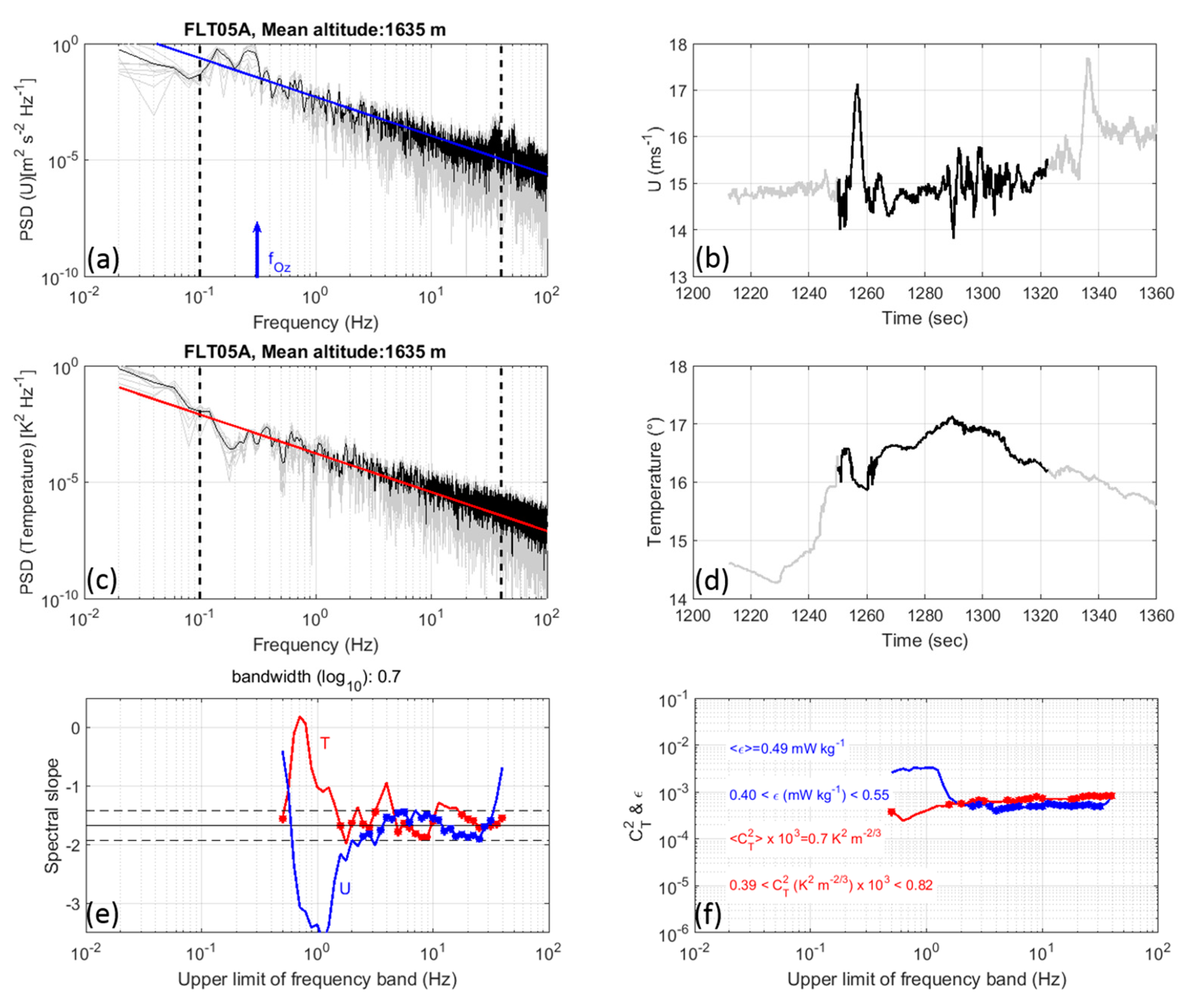
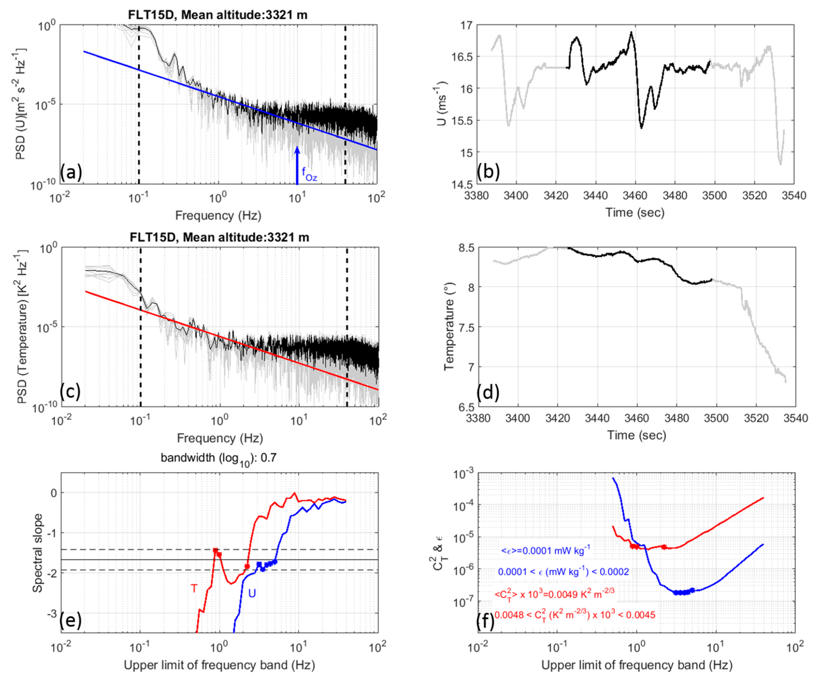
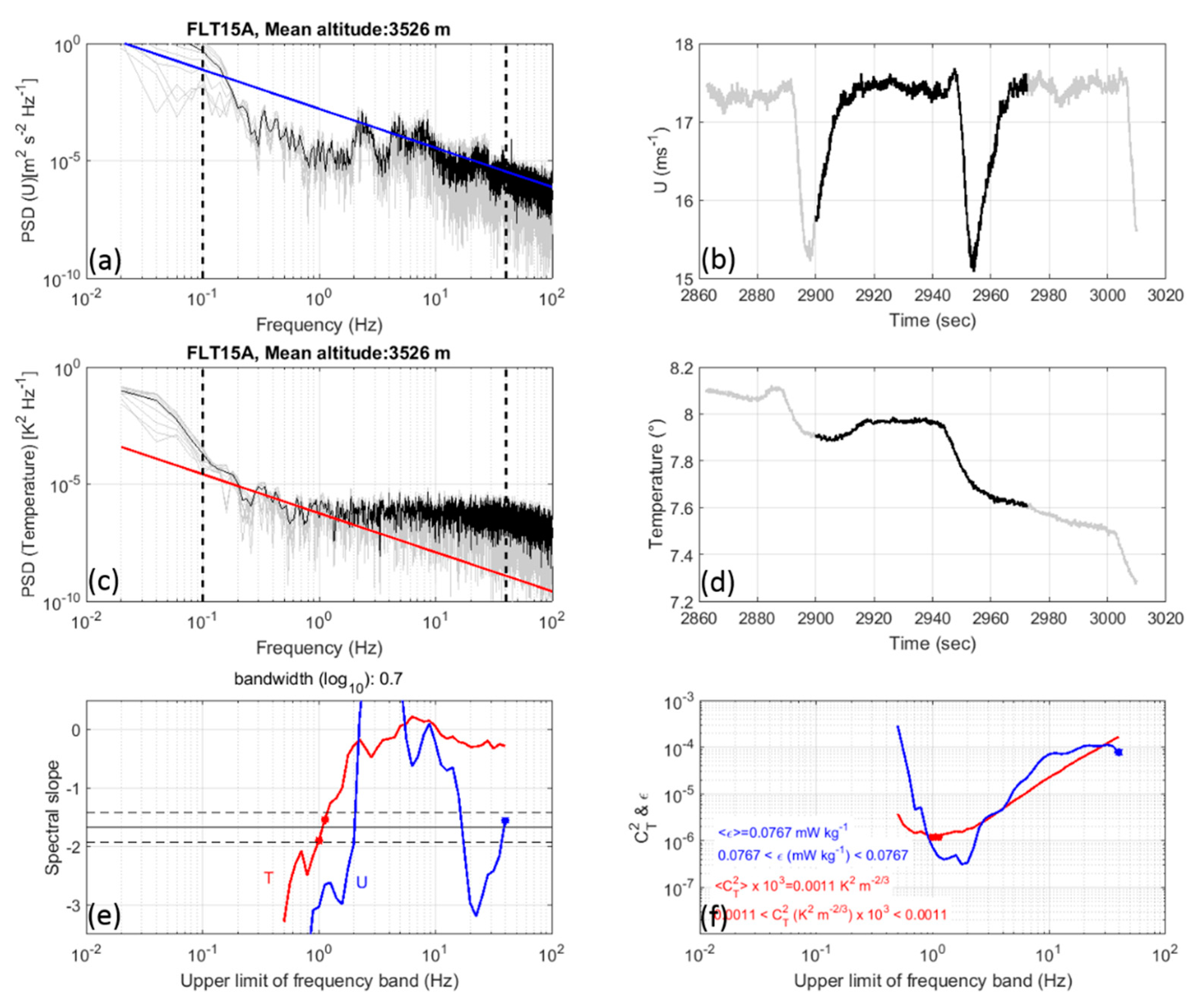
Three examples illustrating the method are shown in Figure 2, Figure 3 and Figure 4. Frequency spectra and the corresponding time series are plotted in panels (a) and (b) for U and (c) and (d) for T, respectively. Panel (e) shows the estimated spectral slope of T and U spectra, as a function of the upper limit f m a x of the frequency band (in l o g 10 scale). For example, f m a x ( 1 ) = 0.5 Hz corresponds to the band 0.1 to 0.5 Hz, f m a x ( 39 ) = 40 Hz corresponds to the band 7.8 to 40 Hz. The values of slopes that meet the selection criterion are indicated by filled circles. Panel (f) shows the corresponding values of ε and C T 2 for each band. The selected values are emphasized by filled circles. The numerical values of the average, minimum and maximum of selected values are also indicated without applying criterion (b) at this stage.
(a) “Strong turbulence”
Figure 2 shows a case from FLT05A for which the −5/3 domain covered a wide frequency range in both T and U spectra. The spectral slopes for f m a x < 2   Hz are rejected because they strongly differ from 5 / 3 , due to a low frequency bump (around 2 Hz ) in U spectra and a corresponding dip in the T spectra. For f m a x > 2   Hz , the T spectral bands show a tendency close to 5 / 3 up to about f m a x = 40   Hz , but they are rejected because the variability of the estimates exceeds ± 0.25 . A less stringent threshold would have enabled us to retain more values, but to the detriment of other cases for which the 5 / 3 tendency is uncertain. Here, spectral bands wider than 0.7 decade would also have provided results that are more satisfying. However, again, it would be to the detriment of cases for which the 5 / 3 domain is much narrower when turbulence is weak. Trade-offs are thus necessary. Here, the non-inclusion of rejected values does not substantially affect the results. For f m a x > 2   Hz , C T 2 estimates do not vary significantly and the average value is close to the value obtained from all values. By using the additional criterion (b), the final C T 2 estimate is made after rejecting the isolated values at f m a x = 0.5, 1.58 and 1.99 Hz and by using the groups of 3, 7 and 9 consecutive values, 19 in total. Here, we find C T 2 ~ 8 × 10 4   K 2 m 2 / 3 after applying (b).
The corresponding U spectral bands show a tendency close to 5 / 3 up to f m a x 30   Hz . The decrease of the slope for f m a x > 30   Hz is due to a narrow and artificial spike just below 40 Hz. The criterion (a) thus permits us to reject the spectral bands corrupted by such contaminations. The average calculated from almost all the values between f m a x = 2.5 and 30   Hz (= 0.49 mWkg 1 ) provides the estimate of ε for the selected time series.
(b) “Weak turbulence”
The spectra shown in Figure 3 and obtained from FLT15A are dominated by instrumental white noise. Both T and U spectra show a slope much steeper than 5 / 3 at low frequencies and close to 0 at high frequencies. For T (U) spectrum, a 5 / 3 domain may be observed for 0.7 < f m a x < 2   Hz ( 2 < f m a x < 6   Hz ). The criterion (b) is met for the U spectrum since there are 5 consecutive values and a very small averaged value of ε = 10 4   mWkg 1 is obtained, but not for T spectrum. This is a typical case for which it is difficult to identify with certainty the presence of an inertial domain, because steeper and gentler slopes are observed at low and high frequencies, respectively.
(c) “Strong instrumental contamination”
The U spectrum shown in Figure 4 and estimated during FLT15A exhibits obvious instrumental contaminations. The T spectrum was free of artificial spikes. The application of criteria (a) and (b) lead to undefined values of ε and C T 2 due to contaminations and instrumental noise, respectively. Figure 4b shows an unusual case, however. The 50 s time series of U and T show dips and steps probably due to a steep bank and sudden loss of altitude. However, these fluctuations are not the cause of the artificial spikes above 10 Hz in the U spectra.

3.4. Attempt at Interpretation of the −5/3 Subranges in Terms of Kolmogorov Turbulence

The consistency of the observed −5/3 domain with the assumptions for Kolmogorov inertial range theory can be inferred from the estimation of the Ozmidov length scale L O . It is defined as:
L O = ε N 3
Its inverse k O defines a wavenumber indicative of the separation between the Kolmogorov inertial and buoyancy subranges. The corresponding Ozmidov frequency f O z can be defined as U ¯ / ( 2 π L O ) . It is expected to be indicative of the lower limit of the inertial subrange in the U frequency spectrum. Its definition differs from that given by Frehlich et al. [13] and Kit et al. [14] for example, by a factor 2 π . Here, this factor is justified by the fact that L O is not a wavelength, but a scale, and that k O = ( 2 π / U ¯ ) f O z = 1 / L O . However, the results discussed here are not strongly dependent on this factor.
f O z is estimated from ε using the method described in Section 3.2 and from N 2 estimated as follows: for an ascent or descent rate of ~2 ms 1 , each temperature data segment corresponds to a vertical segment Δ z of (~2x50 s) = 100 m. The corresponding temperature variation Δ T is estimated after a linear interpolation of the measured temperature profile. Then:
N 2 g T ¯ ( Δ T Δ z + g c p ) ,
where T ¯ is the mean temperature within the segment and c p = 1004   Jkg 1 K 1 . The same procedure is used when assessing the relevance of Equation (1) in Section 4. Equation (10) is relevant if | W / W U A V | 1 where W and W U A V are the vertical air and UAV velocities, respectively (see Appendix A). During the UAV flights, this condition was mostly fulfilled in the free atmosphere according to MU radar measurements of vertical air velocities. However, it must be kept in mind that vertical air motions can be a source of errors on N 2 that should increase the dispersion of the statistical distributions of the turbulence parameters depending on N 2 and shown in Section 4.
The values of f O z are indicated on Figure 2 and Figure 3. For the “Strong turbulence” case (Figure 2), ε 5 × 10 4   m 2 s 3 , N 2 4.5 × 10 4   rad 2 s 2 , L O 7 m, f O z 0.3 Hz. The −5/3 behavior observed for higher frequencies is thus consistent with the hypothesis of a Kolmogorov inertial subrange. For the “Weak turbulence” case (Figure 3), ε 10 7   m 2 s 3 , N 2 1.4 × 10 4   rad 2 s 2 , L O 0.25 m, f O z 10 Hz. The portion of the spectrum exhibiting a −5/3 slope was found at lower frequencies ( 2 < f m a x < 6   Hz ) in the U spectrum and f O z is within a frequency domain dominated by the instrumental noise. Therefore, it is not consistent with Kolmogorov inertial turbulence. This result raises issues about the interpretation of the −5/3 domain in this case. If a −5/3 slope is not a signature of Kolmogorov turbulence (as discussed in 3.3a), ε would be overestimated and f O z would be underestimated, reinforcing the conclusion. If it is relevant, another regime must be considered. Stratified turbulence at low Froude number ( F r = σ U / N L 1 , where σ U is a velocity scale and L the corresponding horizontal velocity scale) consisting of quasi-horizontal turbulent motions may lead to the presence of inertial subranges in horizontal spectra at scales larger than the Ozmidov scale [37,38]. In stable boundary layers, dynamical processes strongly affected by the stable stratification can lead to various regimes producing −5/3 or shallower slopes at scales larger or smaller than the Ozmidov scale [14,38]. The identification of −5/3 domain associated with non-Kolmogorov regime may lead to erroneous estimates of ε and C T 2 , unless there is no spectral gap between the two regimes (as in the case reported by Frehlich et al. [13]).
The statistical results described later on in Section 4 do not seem to indicate a posteriori a noticeable misinterpretation with non-Kolmogorov inertial regimes.

3.5. Additional Evaluation of the Processing Methods

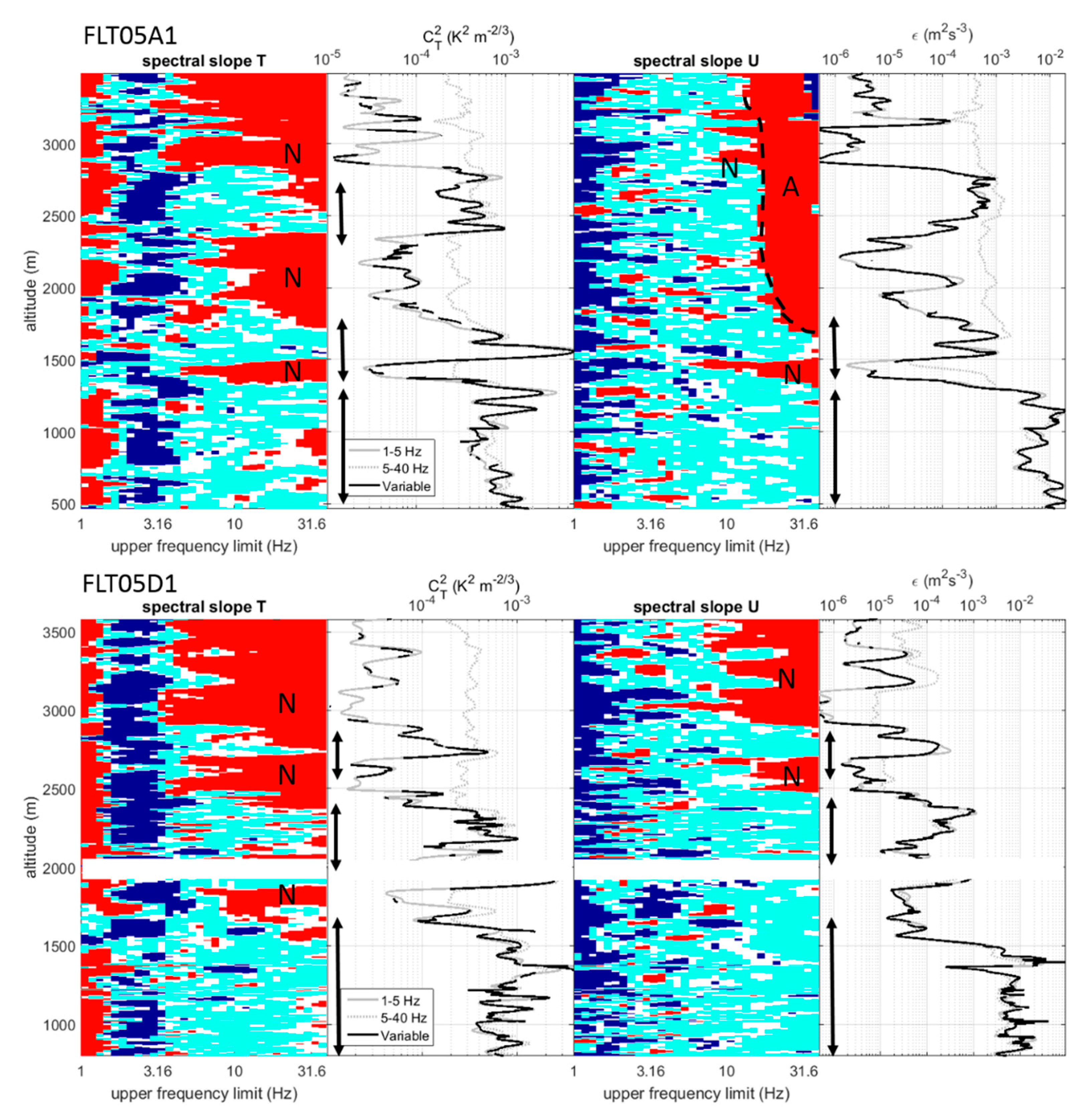
Figure 5 shows two dimensional plots of the T and U spectral slopes for 1 < f m a x < 40   Hz in log 10 scale and for all the spectra during FLT05A and FLT05D. The corresponding profiles of C T 2 and ε estimated, (1) after application of criteria (a) and (b), (2) from the band [1–5 Hz] and (3) from the band [5–40 Hz] are shown at the right side of each plot. For better legibility, only three levels of colors are shown corresponding to three ranges of slopes: p < 5 / 3 0.5 (blue), 5 / 3 0.25 < p < 5 / 3 + 0.25 (cyan) and p > 5 / 3 + 0.5 (red), with a gap of 0.25 between each range for a clear distinction. The steep slopes displayed by the blue levels at low frequencies (for f m a x <   3   H z ) may have an instrumental (unknown) origin and should not be considered. The morphology and intensity of the corresponding spikes strongly depend on the UAV flights (not shown).
As expected, the spectral extent of the inertial domains is large when C T 2 and ε values are high, as emphasized by black vertical double arrows in Figure 5. Most of the red levels at the right side of the 2-D plots, labeled ‘N’, should be understood as the effect of the instrumentation noise. For U spectra and during FLT05A, a spectral contamination by narrow spikes affects the spectra down to 20 Hz. An example was shown in Figure 2 where a spike appears below 40 Hz at the altitude of 1635 m. The contaminations drift toward lower frequencies with time/altitude. The contaminated region is delimited by a thick dashed line and is labeled ‘A’ in Figure 5. In the top-right-hand corner of the 2-D plot, the blue region (steep slopes) indicates that the spectral band was on the right side of the spike. The criteria used permitted us to avoid this contamination when estimating ε . C T 2 and ε values are low or not defined, when the inertial domains are found to be very narrow: the ‘red’ domain is largely extended toward the low frequencies. As the CWT data are relatively noisier than the Pitot data, the C T 2 profiles usually exhibit more undefined values than the ε profiles. The values from the band 5–40 Hz are often strongly overestimated due to instrumentation noise (e.g., around 3000 m during descent for ε and above ~1500 m for C T 2 during ascent and descent) and due to artifacts (above 1700 m during ascent for ε ). FLT05 reveals substantial turbulence at all altitudes. Other flights (as FLT28, see Section 4.3) showed weak turbulence and many more estimates were undetermined after application of the criteria (a) and (b).
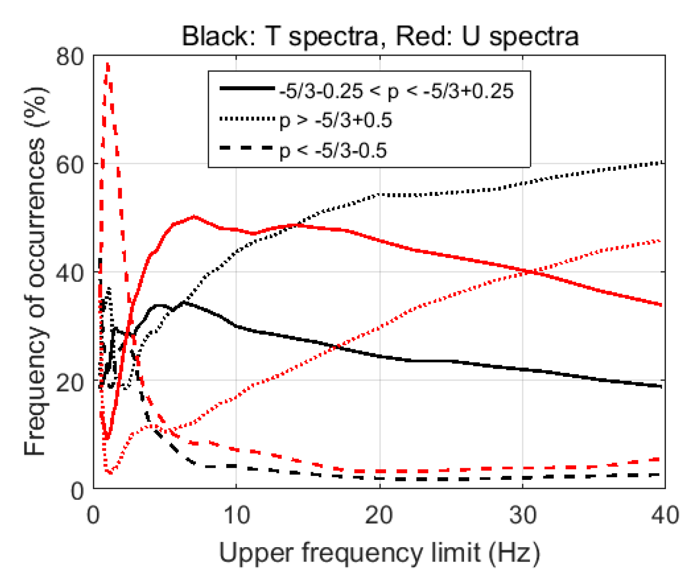
The frequencies of occurrence of ranges of slopes for T (black) and U (red) spectra are shown in Figure 6. The largest occurrences of 5 / 3 0.25 < p < 5 / 3 + 0.25 (a qualified inertial domain) are found for 5 < f m a x < 8   Hz , i.e., for frequency bands of 1-5 Hz to 1.6-8 Hz (~35 % for T spectra, 50 % for U spectra). This frequency range was used by Luce et al. [19] for estimating ε from Pitot data to be compared with MU radar estimates of ε . Above f m a x   8   Hz , the frequencies of occurrence slowly decrease down to 20% and 35% at f m a x = 40   Hz for T and U spectra, respectively, because of instrumentation noise and artifacts. The frequencies of occurrence of p > 5 / 3 + 0.5 (spectra affected by noise and artifacts) monotonically increase with f m a x . They reach 60% and 45% at f m a x = 40   Hz and should still increase for higher frequencies. Even if the frequency of occurrences of p < 5 / 3 0.5 (spectra affected by artifacts apart from the low frequencies) does not exceed ~5% (with a slight increase with as f m a x increases), the quantitative effects can be large because the spikes are generally very energetic (see Figure 5). It is thus important to remove their contribution as much as possible.

4. Results of Analyses

4.1. Estimation of γ

γ Equation (2) can be estimated from Equation (1):
γ = T 2 g 2 N 2 ε 2 / 3 C T 2 ,
where N 2 is estimated using Equation (10). ε and C T 2 values associated with convectively generated turbulence and cloudy air must be, in principle, discarded. This was done when:
(1) Relative humidity measured by the humidity sensor on board the UAV exceeded 85%. This threshold is rather arbitrary and may be affected by inaccurate calibration of the humidity sensors. It may lead to discarded data in clear air conditions under some occasions, without impact on the statistical results. In practice, cloud particles can often be observed even when the relative humidity is below but close to 100%, depending on altitudes, and radiosondes [39].
(2) The data were associated with convective boundary layers (CBL). These often extended up to the altitude of 2000–2500 m at midday during sunny periods. They were easily identified from MU radar observations, when CBL top reached the minimum observable altitude, i.e., 1270 m (for example, Figure 23 of Kantha et al. [18]). From temperature and humidity data, CBL is usually weakly stratified and capped by a sharp temperature inversion associated with a relative humidity decrease. In addition, CBL is generally associated with the largest values of ε and C T 2 . All these features helped us identify the vertical extent of CBL.
(3) Turbulence was caused by convective instabilities underneath mid-level cloud base (MCT) [40]. Very few such cases were probed, because the MCT often occurred at altitudes unreachable by the UAVs.
These criteria disqualified 24.7% of the estimates made from the 39 flights. The remaining data are expected to fit the assumptions underlying Equation (1), because the main sources of convection due to thermodynamic effects were excluded. Among the discarded data, an overwhelming majority comes from the CBL, which was sometimes partly cloudy. In the following, we will attribute all the discarded data to CBL for simplicity. Some of the estimates for CBL data were de facto discarded when N 2 was locally negative so that Equations (1) or (11) cannot be applied. The temperature profiles in CBL sometimes revealed suspicious, successive and almost periodic superadiabatic and stable gradients. Their origin is unclear but, for at least some of the observed cases, they could be produced by the possible presence of strong updrafts or downdrafts in the convective cells (see Appendix A). A possible similar effect reported in a review by Gossard [41] was observed from tower measurements during strong buoyancy wave perturbations.
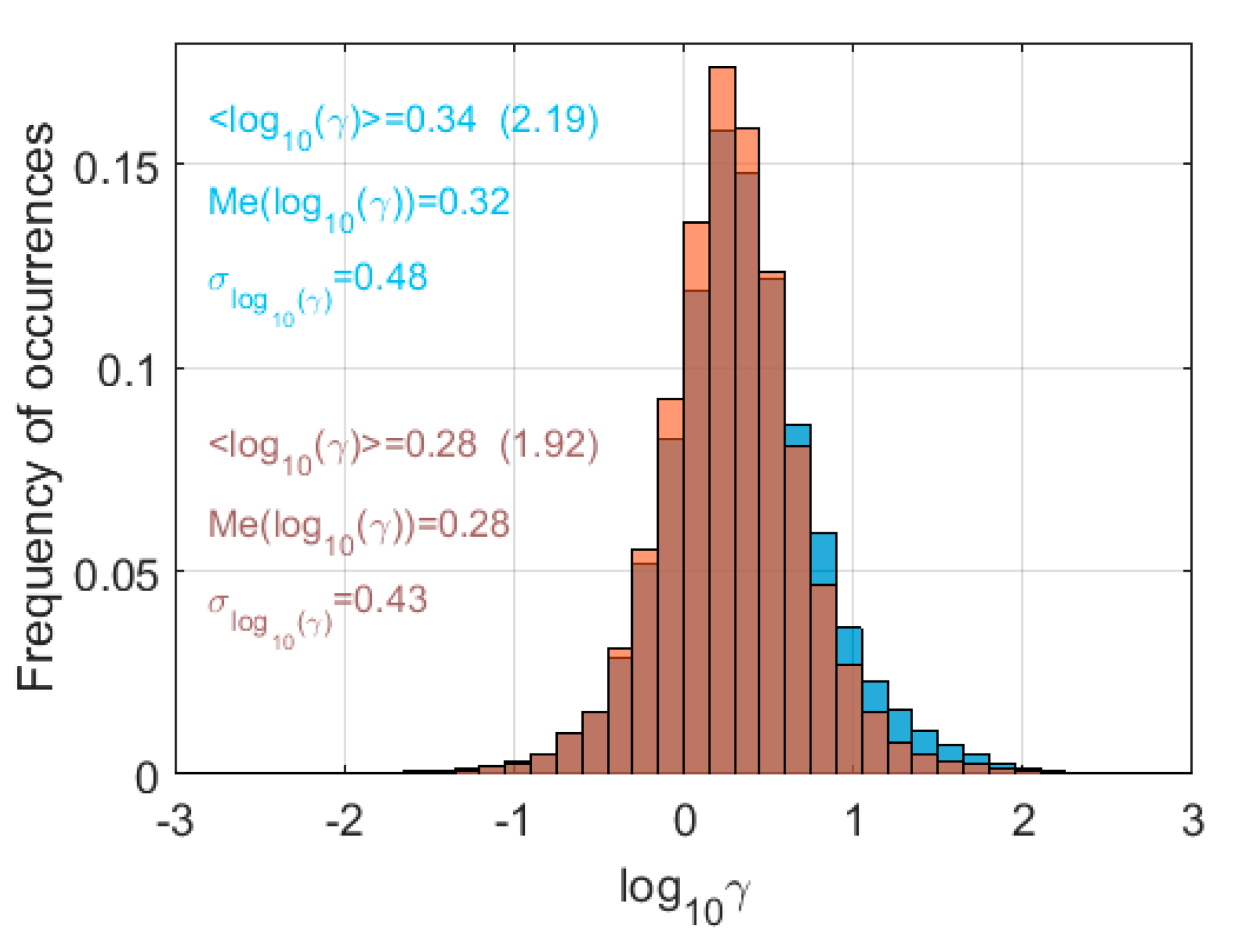
Without CBL data, the distribution of frequency of occurrences of l o g 10 ( γ ) obtained from the 39 flights has a nearly log-normal distribution with identical mean and median values of 0.28 for l o g 10 ( γ ) and 1.92 for γ (Figure 7). This value is close to 1.95 obtained from ShUREX 2016 data only [21]. The standard deviation σ l o g 10 ( γ ) of the distribution is 0.43 and the percentage of values that lie within the band < l o g 10 ( γ ) > ± σ l o g 10 ( γ ) is 75% (68% for a normal distribution). Therefore, the distribution clearly indicates the existence of a preferential value of γ around 1.92. This value significantly differs from typical values sometimes used by default in the literature of atmospheric studies. γ 1.0 was used by Gavrilov et al. [3] based on the assumption of R f = 0.25 . Using slightly different models, γ 0.4 was proposed to be used by Hocking [34]. This is smaller than our estimate by a factor ~5 and would produce a factor ~ 11 between ε and ε C T 2 .
Including CBL data, the distribution is slightly shifted and skewed to the right (Figure 7). The mean and median values of l o g 10 ( γ ) are 0.34 and 0.32, respectively. The distribution is more spread out than the distribution obtained excluding the CBL ( σ l o g 10 ( γ ) = 0.48 ). Therefore, CBL data make a significant contribution to the statistics and can be a source of bias when evaluating γ . In the following, we will focus on the statistics made from data outside the CBL. A detailed analysis of the relationship between ε and C T 2 in convective and cloudy regions remains the subject of future studies.

4.2. Estimations of ε C T 2 , χ m and R f

We compared ε to ε C T 2 by using < l o g 10 ( γ ) > = 0.28 with N 2 estimated from Equation (10), and < N 2 > = 1.47 × 10 4   rad 2 s 2 (Figure 8a). The constant value < N 2 > is the average of N 2 for selected height ranges in stratified and clear air conditions. The scatter plots show ε and ε C T 2 vary between ~ 10 7   m 2 s 3 and ~ 10 2   m 2 s 3 . The regression slope is close to 1 for both measured and averaged N 2 (1.11 and 1.17, respectively). It slightly exceeds 1 partly because of a slight asymmetry of the scatter plot for weak values of ε and ε C T 2 ( 10 6   m 2 s 3 ) . Rather than a different property of turbulence for weak values, this feature may result from imperfections of the rejection/selection procedure described in Section 3 and should probably not be taken into account. The scatter is more important with < N 2 > than with N 2 and the correlation coefficients are 0.74 and 0.81, respectively. An increase of the dispersion and a decrease of the correlation when using < N 2 > suggest that the N 2 estimates from Equation (10) are meaningful and are thus more representative than the average value. The use of an average or standard N 2 value cause significant disagreements for individual cases as shown later on, in Section 5.
The histograms of mixing coefficient χ m and flux Richardson number R f (in l o g 10 scale) cover about two orders of magnitude (Figure 8b,c). Their mean and median values obtained from N 2 and < N 2 > do not differ significantly: 0.16–0.17 and 0.13–0.15, respectively. As mentioned by [21], these values are close to the canonical values of χ m =   0.2 and R f =   0.17 reported in the literature on oceanic turbulence [22] and theorized by Ellison [23]. The fact that the upper tail of the distribution of l o g 10 ( χ m ) exceeds 0 (i.e., χ m exceeds 1) indicates that the distribution is affected by statistical estimation errors, in particular on N 2 , that make it even wider than it should be. Considering that these distributions are also conditioned by the validity of Equation (1), it is not possible to infer the real variability of χ m and R f . Interestingly, the spread of the distribution of R f obtained for oceanic turbulence from different methods and with accurate evaluations of parameters [22] is very similar to that shown in Figure 8c.

4.3. Examples of Profiles

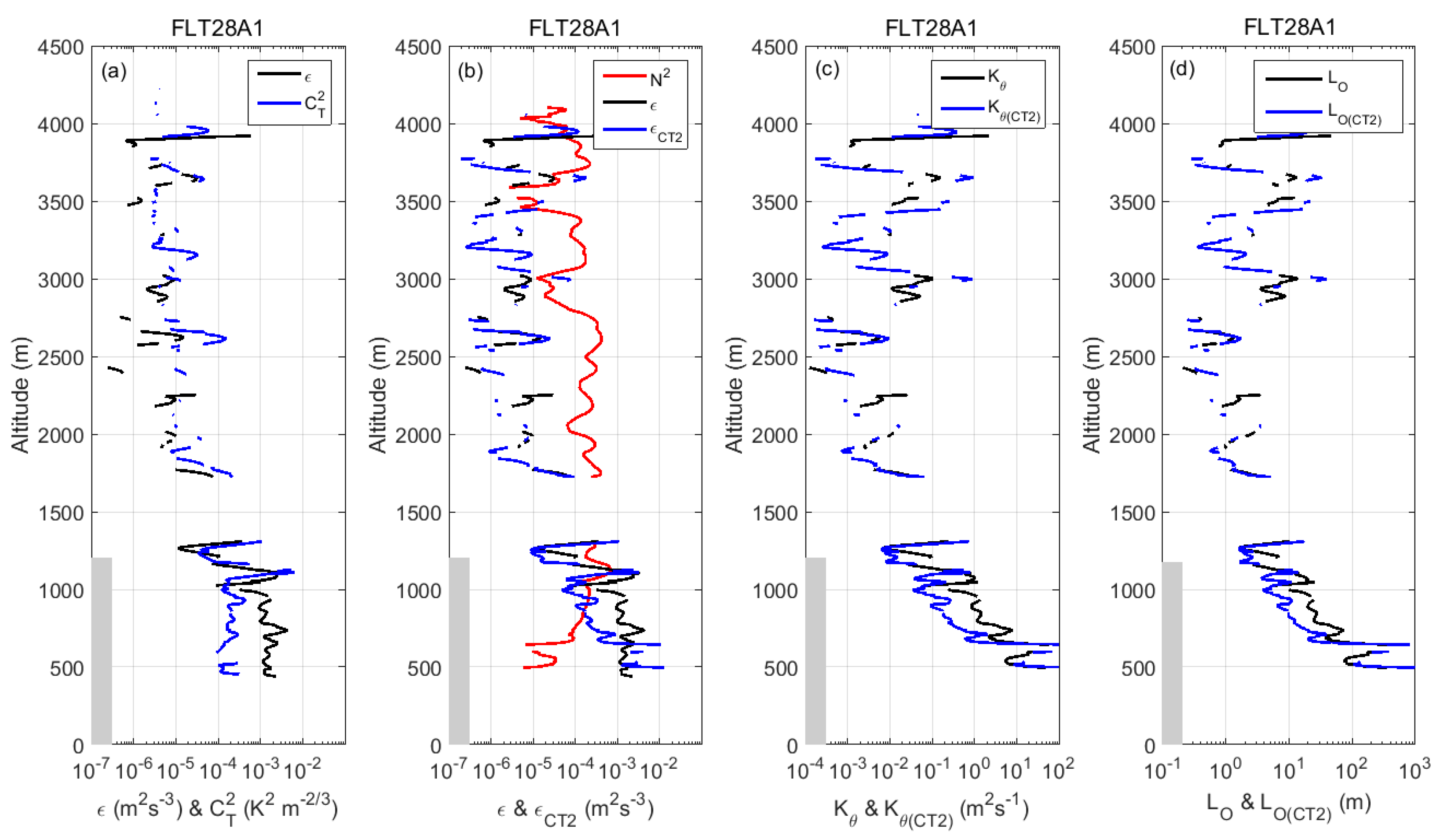
We inferred (pseudo) vertical profiles of turbulence parameters and some examples are shown in Figure 9, Figure 10 and Figure 11 for FLT05A1, FLT28A1 and FLT40A1, respectively. We note the Ozmidov scale L O ,   L O ( C T 2 ) and the eddy diffusivity K θ ,   K θ ( C T 2 ) inferred from ε and ε C T 2 , respectively. K θ   and   K θ ( C T 2 ) were estimated from Equation (3) using < R f / ( 1 R f ) > = < χ m > = 0.16 . This value is smaller by a factor 2 with respect commonly used formulas assuming R f   = 0.25 [2,24] and by a factor 5 with respect to Hocking [42] and a factor 2.5 with respect to Hocking [43].
The altitude ranges associated with CBL in Figure 9 and Figure 10 show the largest discrepancies between the profiles because Equation (1) should not apply. On the day of FLT40, CBL did not form but cloudy air (relative humidity=100%) was observed up to ~1900 m (Figure 11). In the height range 1200–1800 m, ε C T 2 ( K θ ( C T 2 ) ,   L O ( C T 2 ) ) strongly underestimate ε ( K θ ,   L O ) by up to two orders of magnitude, whereas there is a good agreement below 1200 m. This observation might indicate that air saturation is not always a sufficient criterion for faulting the validity of Equation (1). The discrepancy in the height range 1200–1800 m is clearly not due to statistical errors and is one of the rare prominent cases not related to CBL at odds with the model. The hypothesis of vanishing temperature turbulence due to strong mixing [44] for stratospheric heights (their Figure 1 and Figure 2) can be discarded because this hypothesis implies enhancements of C T 2 and N 2 at the edges of the mixing layer and a decrease of N 2 at the center. These characteristics are not observed here (Figure 11b).
Above CBL and outside cloudy regions, Equation (1) with < l o g 10 ( γ ) > = 0.28 is applicable because the profiles are consistent with each other. The largest discrepancies result mainly from differences between the amplitudes of the peaks (e.g., at the altitude of 1700 m in Figure 9 where the ratio is 10 for the 3 parameters).
In Figure 9, the profiles reveal an alternation of peaks of dissipation rates, whose depths vary from 100 m or less (at 3200 m) up to 600 m around 2600 m (hereafter denoted T1). In the latter case, ε and ε C T 2 reached 10 3   m 2 s 3 , K θ and K θ ( C T 2 ) exceeded 1.0 m 2 s 1 and L O and L O ( C T 2 ) exceeded ~20 m. Deep minima (or undetermined values) were observed at 1400, 2200 m and around 3000 m.
In Figure 10, turbulence was weak above the CBL, and only a few isolated and thin layers were probed (data were missing around 1500 m). The depth of the peaks did not exceed ~100 m typically. ε and ε C T 2 values did not always coincide, but there were likely significant peaks at 2000, 2600, 3700 and 4000 m with ε and ε C T 2 ~ 10 5   m 2 s 3 , K θ and K θ ( C T 2 ) ~ 10 2 10 1 m 2 s 1 and L O and L O ( C T 2 ) ~   1   10   m .
In Figure 11, the noticeable feature is the thick layer of enhanced turbulence parameters between 2200 and 3000 m (hereafter denoted T2). ε and ε C T 2 reached 10 3   m 2 s 3 , K θ and K θ ( C T 2 ) exceeded 1.0 m 2 s 1 and L O and L O ( C T 2 ) exceeded 50 m. There were also sharp peaks of ε and ε C T 2 ( ~ 5 × 10 5   m 2 s 3 ), K θ and K θ ( C T 2 ) ( ~ 8 × 10 2   m 2 s 1 ) and L O and L O ( C T 2 ) ( ~   5   m ) at 2000 m embedded within two deep minima.
In T1 and T2, C T 2 and ε are both enhanced. This differs from that reported by Bertin et al. [44] for stratospheric layers because ε was enhanced where C T 2 was minimum. The difference may suggest an earlier stage of turbulence and/or another model of evolution. A careful inspection of the overall profiles did not reveal events similar to those shown by Bertin et al. [44] in stratified conditions.

4.4. Statistics for K θ and L O

< K θ > = 0.03   m 2 s 1 and < L O > ~ 4   m was obtained for both N 2 and < N 2 > (Figure 12). These values are consistent with those reported from balloon data collected at stratospheric heights [29,44]. However, 6.7% of K θ values exceeded 1.0 m 2 s 1 (e.g., T1 and T2 of Figure 9 and Figure 11), indicating that some of the observed turbulent events may have had a much more significant impact in terms of diffusion than those reported in the literature [29,44].
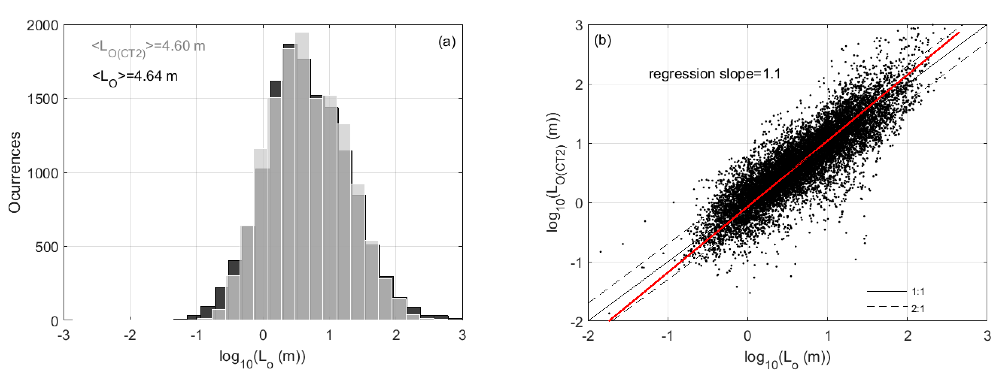
Figure 13 shows distributions of l o g 10 ( L O ) and l o g 10 ( L O ( C T 2 ) ) and a scatter plot of l o g 10 ( L O ) vs. l o g 10 ( L O ( C T 2 ) ) with a regression line. The averaged values differ slightly from those shown in Figure 12, because the average was calculated when L O and L O ( C T 2 ) are both available. Both distributions show very similar shapes and 71% of the Ozmidov scale estimates agree within a factor less than 2.
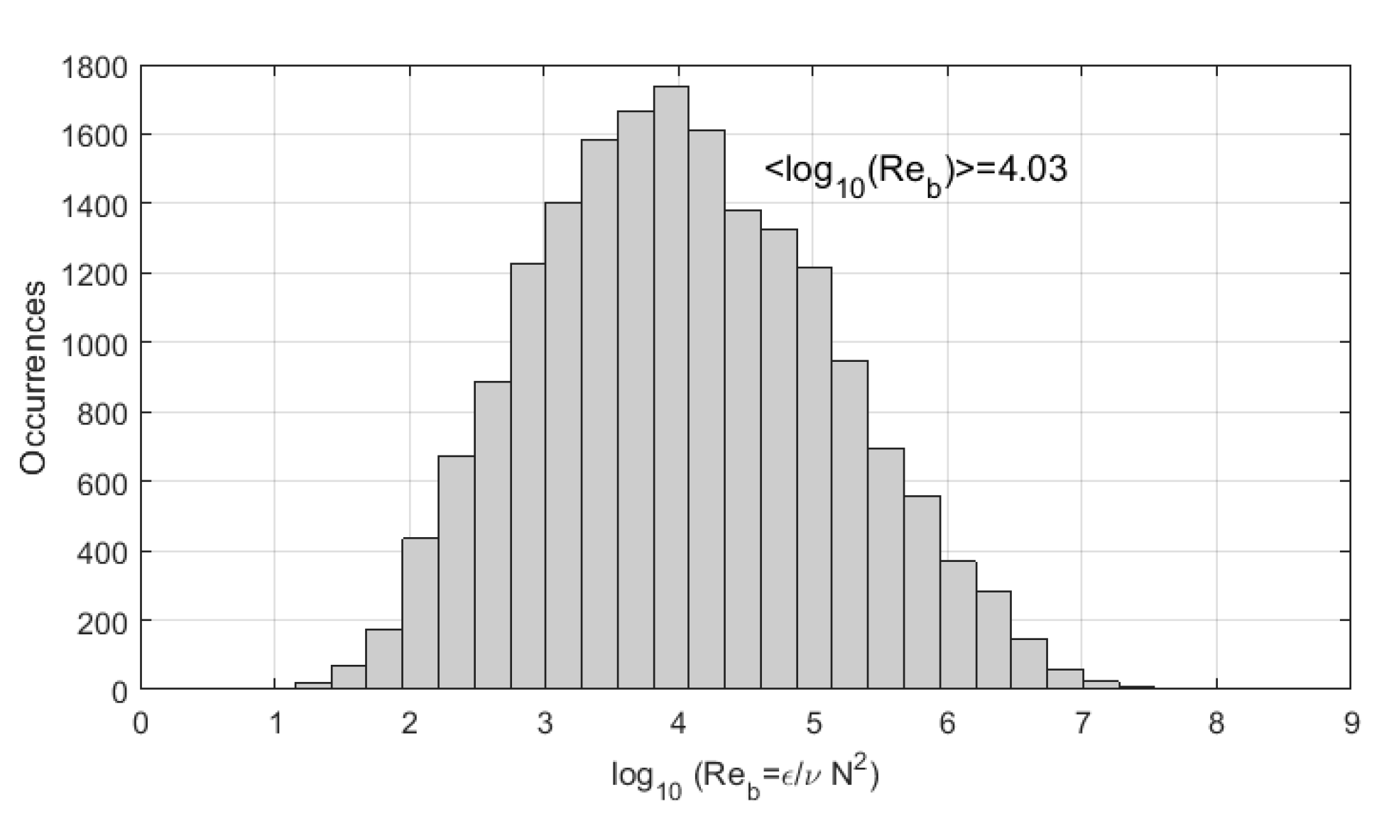
Finally, Figure 14 shows the distribution of the buoyancy Reynolds number R e b = ε / ( ν N 2 ) = ( L O / η ) 4 / 3 ,   in l o g 10 scale, where ν is the molecular kinematic viscosity and η is the Kolmogorov length scale. The average value of l o g 10 ( R e b ) is ~4.0 (i.e., the average value of R e b is ~10,000) and 95% of the estimates fulfill the condition R e b > 200 , consistent with isotropic turbulence according to [45] for oceanic turbulence. It is an additional clue that our qualified estimates of ε are meaningful and related to Kolmogorov turbulence.

4.5. Shear and Richardson Number

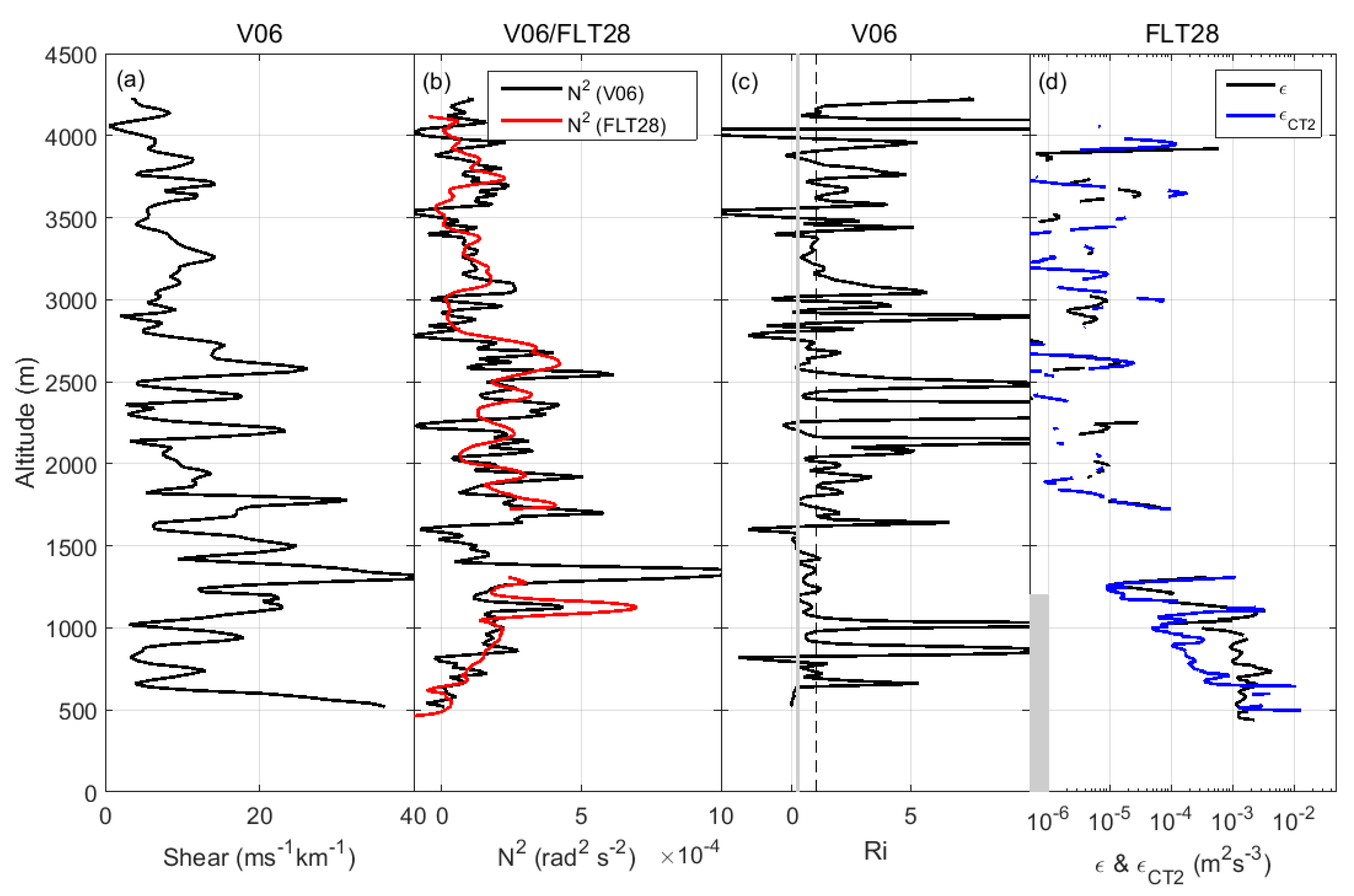
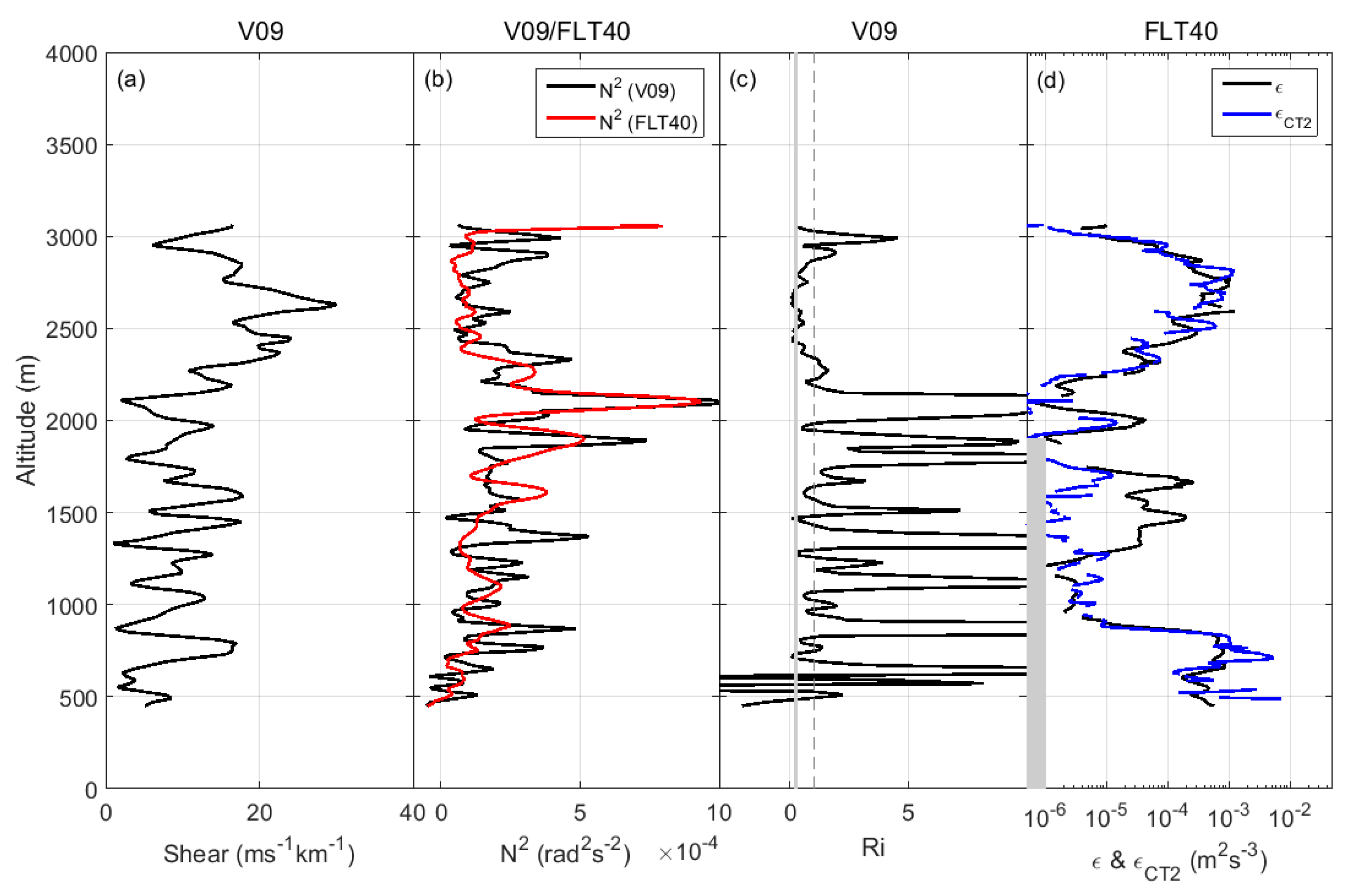
A clear relationship between enhanced turbulence parameters and both enhanced shear S = ( ( d u / d z ) 2 + ( d v / d z ) 2 ) 1 / 2 where u and v are the zonal and meridional wind components and small gradient Richardson number R i = N 2 / S 2 was reported from UAV data up to altitudes of ~500 m [17]. The estimation of wind shear and R i from UAV measurements is still under consideration for ShUREX data. However, these parameters can be obtained from RS92G Vaisala radiosondes launched on some occasions from the observatory concurrently with the UAVs. Two radiosondes (hereafter called V06 and V09) were launched around the flights FLT28 and FLT40 described in Section 4.4. V06 was launched about 30 min before FLT28 and drifted horizontally by 5600 m at the maximum altitude of FLT28. V09 flew almost simultaneously to FLT40. V09 drifted horizontally by about 7700 m at the maximum altitude of FLT40.
We first compared N 2 profiles derived from radiosonde and UAV data, hereafter denoted N 2 ( V ) and N 2 ( F L T ) , respectively, where “**” is the flight number, for checking their consistency (Figure 15 and Figure 16). N 2 ( V 06 ) and N 2 ( F L T 28 ) compare quite well (Figure 15b). Altitudes of V09 data were shifted downward by 130   m in order to correct a vertical offset between the most prominent peak of N 2 ( V 09 ) and N 2 ( F L T 40 ) at ~2150 m. After this correction, N 2 ( V 09 ) and N 2 ( F L T 40 ) profiles also show very similar features (Figure 16b). We thus assume that the shear and R i values estimated from V06 and V09 data are also representative, at least qualitatively, of the dynamical conditions met during FLT28A1 and FLT40A1.
For FLT28A1, the R i profile fluctuates with height with alternating large values ( R i > 10 ) and small values ( R i < 1 ) in the stratified region above the altitude of 1700 m. It is qualitatively consistent with the sporadic peaks of ε and ε C T 2 (Figure 15d). The narrow peak of ε and ε C T 2 around ~2150 m (Figure 15d) is associated with R i < 0.25 (Figure 15c) and a shear maximum of ~ 20   m s 1 k m 1 (Figure 15a). For FLT40A1, the maxima of R i   ( > 10 ) at 1800, 2200 and 3000 m coincide with the minima of ε and ε C T 2 or even undefined values (Figure 16d). The thick turbulent layer (T2 in Figure 11) with enhanced ε and ε C T 2 (Figure 16d) coincides with a deep minimum of R i ~ < 0.25 (Figure 16c) and shear maximum of ~ 20   ms 1 km 1 (Figure 16a). All these observations are consistent with the commonly accepted criteria on gradient Richardson number for turbulence generated by dynamic shear instabilities and confirm results described by Balsley et al. [17]. It is again an additional clue supporting the hypothesis that we truly selected 3-D Kolmogorov turbulence rather than stratified turbulence.

5. Analysis of a Data Segment

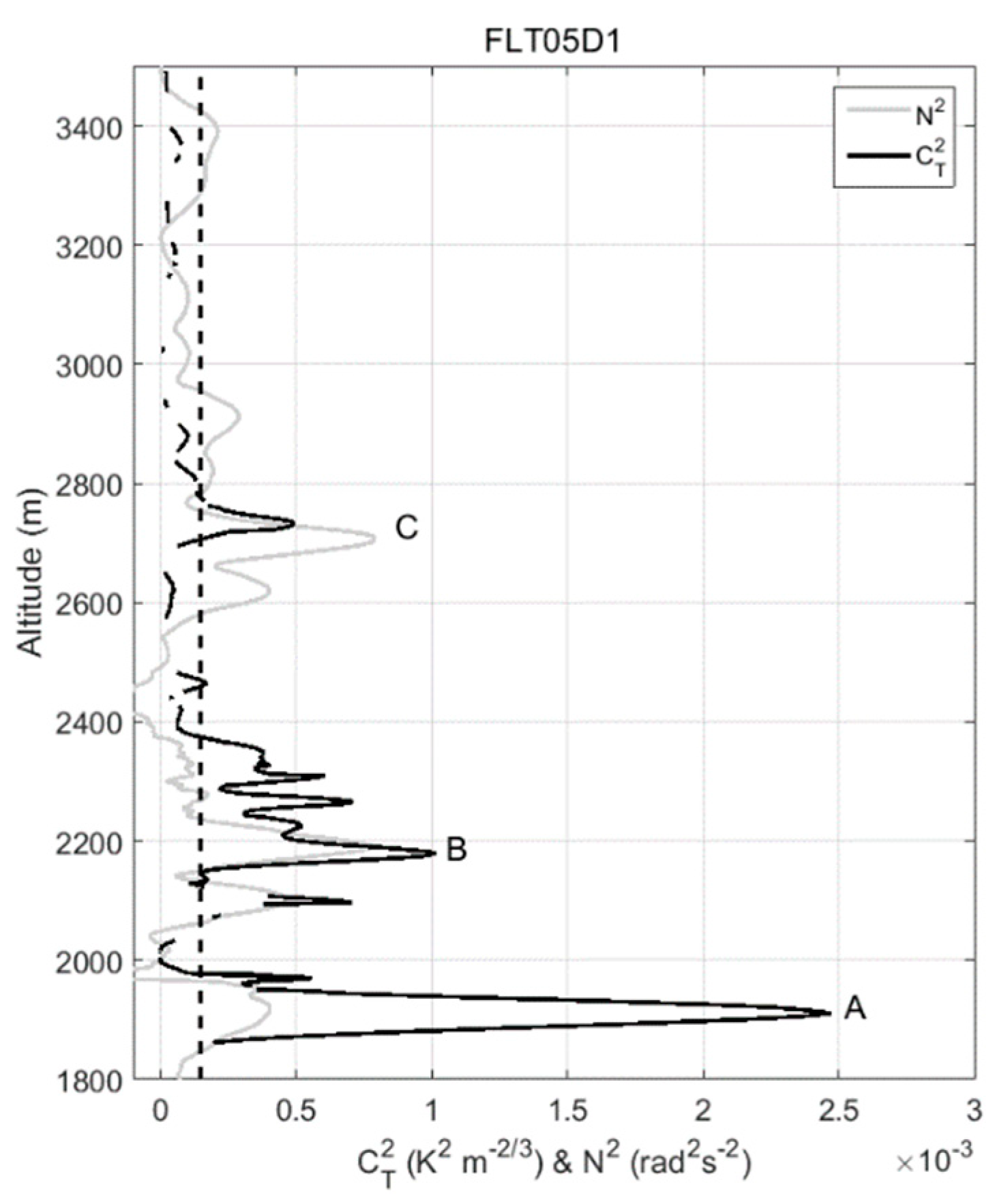
Here, we mainly describe a case-study selected from FLT05D1 (Figure 5). The profiles of C T 2 and N 2 show noticeable similarities and differences in the height range 1800–3500 m (Figure 17). Below the altitude of 2400 m, several peaks of C T 2 exceed 5 × 10 4   K 2 m 2 / 3 and N 2 generally exceeds the mean value of 1.47 × 10 4   rad 2 s 2 with peaks up to 8 × 10 4   rad 2 s 2 . Above 2800 m, where N 2 is smaller but exceeds 10 4   rad 2 s 2 in some altitude ranges, C T 2 is minimum or even undetermined. Such properties in both the troposphere and stratosphere from high-resolution balloon temperature data were reported by Gavrilov et al. [3]. The C T 2 peaks labeled A, B and C are closely associated with N 2 peaks. Note how A, B and C differ from T1 (Figure 9) and T2 (Figure 11). The depths of A, B and C are less than ~100 m whereas T1 and T2 are deep (600–800 m) and not associated with a well-defined N 2 enhancement. A careful inspection of the profiles shows that the altitudes of N 2 and C T 2 peaks do not coincide exactly. The differences of altitude, z C T 2 m a x z N 2 m a x for A, B and C are −10 m, −9 m and + 35 m, respectively. The other peaks in Figure 17 have not been selected, because the peak association may be quite arbitrary due to multiple consecutive peaks. In order to check the significance of these vertical offsets, 134 additional cases have been selected from the 39 flights. Great care has been taken to select isolated peaks such as A, B and C. A large majority of the selected cases show a positive or negative offset between N 2 and C T 2 peaks of the order of ± ( 10 30 )   m (Figure 18). Therefore, the largest temperature fluctuations attributed to Kolmogorov turbulence did not occur at the center of the temperature inversion but at one of its margins, and never at both margins. From the selected cases, it was not possible to associate unambiguously a C T 2 peak at one margin with another one at the other margin to form a pair of layers of enhanced turbulence at the edges of a more weakly turbulent layer.
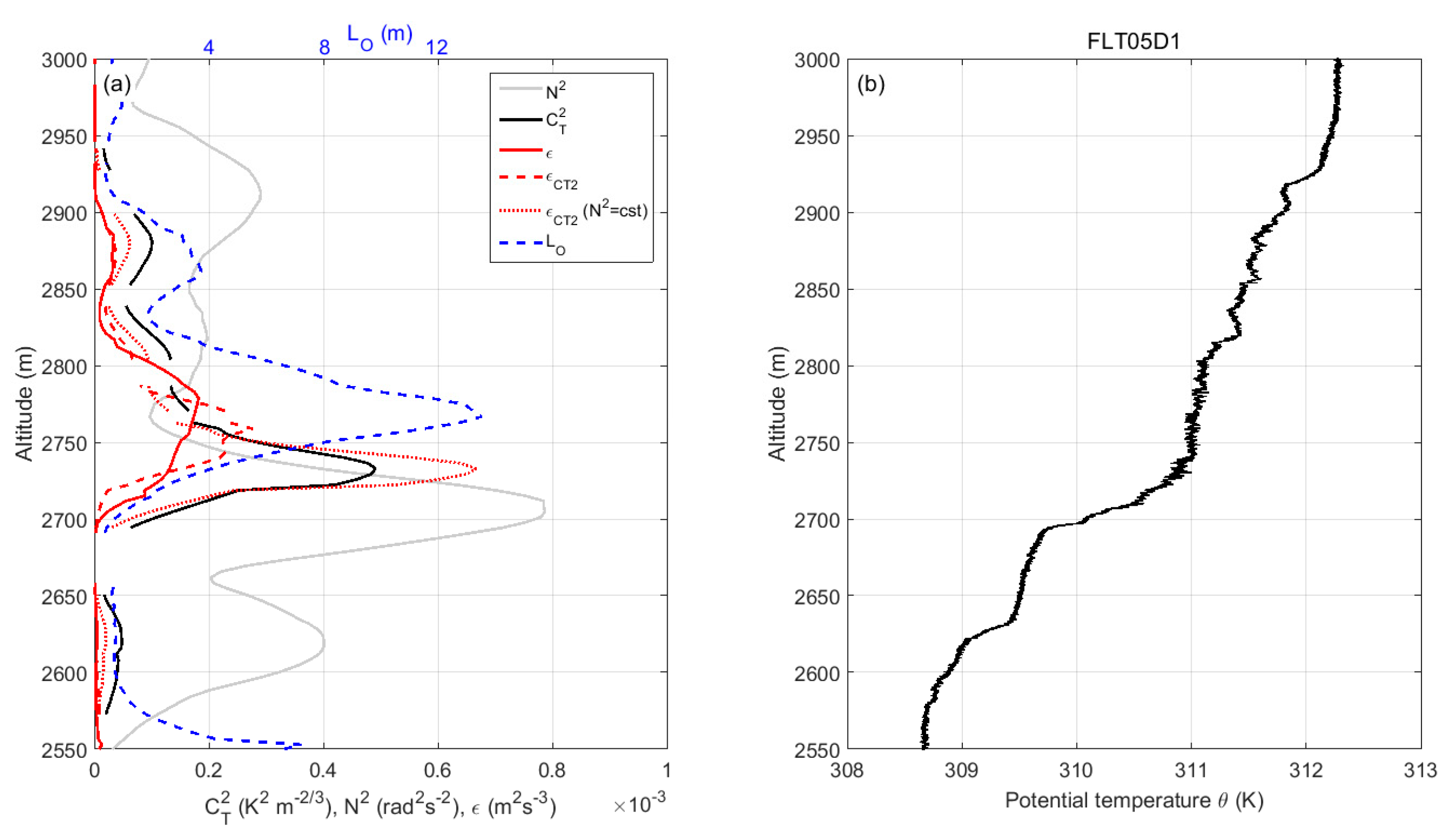
Figure 19 focuses on C, in the height range 2550–3000 m. It shows C T 2 ,   ε , ε C T 2 with N 2 and < N 2 > and L O profiles and the corresponding profile of potential temperature θ . The ε peak is wider than the C T 2 peak and is shifted upward with respect to the C T 2 peak. ε C T 2 and C T 2 obviously coincide when < N 2 > is used and ε C T 2 roughly agrees with ε . However, when using N 2 , the agreement is much better. This particular case illustrates the cause of the statistical improvement when estimating ε C T 2 from N 2 with respect to < N 2 > (Figure 8). The maximum of ε (or ε C T 2 ) above the maximum of N 2 and a maximum of C T 2 between the two is remarkably similar to observations reported by Gossard [41] (Figure 4.5, p. 519), at the bottom of temperature inversions capping the CBL. Thus, mechanisms similar to those observed below capping inversions may occur in the free atmosphere.
The vertical offsets between N 2 ,   C T 2 ,   ε and L O peaks can be interpreted as follows. On the one hand, peak of ε (maximum of Kolmogorov turbulence) is found to be far enough from the center of the stable inversion because the maximum of static stability N 2 inhibits vertical motion (and thus isotropic turbulence). The largest isotropic billows (maximum of L O ) can be observed there. They tend to be smaller when “approaching” the stable inversion, i.e., the Kolmogorov domain tends to be suppressed. On the other hand, large C T 2 requires both enhanced N 2 and ε . When ε ( N 2 ) is maximum, N 2   ( ε ) is reduced so that C T 2 is also reduced. It follows that C T 2 is maximum between ε and N 2 peaks. The level of C T 2 is thus a compromise between the intensity of the dynamic turbulence and the strength of the mean temperature gradient. The potential temperature profile clearly indicates a steep gradient with a laminar appearance at ~2700 m topped by enhanced fluctuations around ~2730 m (Figure 19b).
These observations do not fit into the scheme of a turbulent sheet associated with enhanced C T 2 [16]. A temperature gradient sheet was defined as a temperature inversion of 3–20 m in depth associated with a temperature increase of 0.2–0.8 K corresponding to a gradient of 30–100 K/km [7]. The temperature inversion at ~2700 m (Figure 19b) falls within this definition because the temperature increase is ~0.7 K over ~14 m (gradient ~50 K/km). According to Dalaudier et al. [7], only 29% of the observed temperature gradient sheets in the troposphere and stratosphere were associated with overturning, and thus, potentially enhanced C T 2 . Temperature fluctuations were observed just above or below some sheets but the authors did not explicitly convey turbulence because velocity data were not available at that time. Using identical observation techniques, similar statistics were obtained from data described by Gavrilov et al. [3] (results not published). Our observations are consistent with this type of sheets. They confirm that ongoing mixing (enhanced ε and C T 2 ) is likely not fortuitous at the margins of some temperature sheets and that these sheets may be the result of, or may be reinforced by, turbulent mixing occurring at one of their margins.
This finding can contribute to a longstanding debate about the mechanisms of ground-based clear air radar backscattering. For ST radars operated in the Very High Frequency (VHF) band, echo power is often enhanced in the vertical direction, mainly above the tropopause, but also in the troposphere on some occasions [9]. Partial reflection from thin and horizontally stratified temperature and humidity gradient sheets is often proposed as the primary cause of this phenomenon [9,46]. For radars operated in the UHF band or higher frequencies, the clear air contribution to radar echo power is generally attributed to Bragg backscattering from isotropic turbulence [41]. In stratified conditions, UHF radar echoes also coincide with vertical gradients of temperature and humidity [41]. As a result, time-height cross-sections of VHF and UHF radar echo power do not qualitatively differ at similar range resolutions and both reveal the location of temperature and humidity gradients, when echoes are enhanced. Therefore, a given temperature gradient can be assumed to be either a laminar entity for explaining enhanced VHF radar echoes or a fully turbulent entity for explaining isotropic UHF echoes. Conditions such as those reported in Figure 19 may overcome this paradox. Due to the vertical offset between the temperature sheet and the maximum of C T 2 , the VHF and UHF radar echoes would mainly result from partial reflection from the temperature (and humidity) gradient and scattering from isotropic turbulence at one of its margins, respectively. In practice, the small offset (a few tens of meters or less) would not be enough for distinguishing the difference in altitudes between the VHF and UHF echoes, giving the impression that the same structures are detected. The existence of a small vertical offset between the structures responsible for VHF and UHF radar echoes is an appealing explanation of the paradox, but this explanation requires more thorough investigations, including radar data, for evaluating its relevance and significance.

6. Summary and Conclusions

In the present study, turbulence parameters in the lower troposphere have been estimated using data from high-resolution Pitot velocity and cold wire temperature sensors on board DataHawk UAVs, collected during ShUREX 2016 and 2017 campaigns at Shigaraki MU observatory. The data processing methods used for these estimations have been described in detail. These methods were designed to retrieve reliable estimates of TKE dissipation rate ε and temperature structure function parameter C T 2 from U and T measurements in the presence of measurement artifacts and instrumentation noise. These methods were based on the identification of the inertial −5/3 subranges in 1-D U and T spectra and on the estimation of their levels. Because a slope of −5/3 in (nearly) horizontal spectra can also be a signature of 2-D stratified turbulence for low Froude numbers or high gradient Richardson numbers [13,32], we considered this possibility by comparing the results with properties expected for Kolmogorov turbulence.
(1) The relationship between ε and C T 2 given by Equation (1), valid for Kolmogorov turbulence generated by shear flow instabilities in stratified conditions, was verified after excluding spurious data, confirming the result described by Kantha and Luce [21]. Equation (1) does not work for turbulence in convective boundary layers (e.g., Figure 9 and Figure 10), and leads to puzzling results in saturated conditions with very good agreements or large discrepancies according to altitude ranges (Figure 11). The traditional scheme of local diffusion (K-theory) does not work for convective boundary layers [47] and it can be expected that local stability ( N 2 ) does not contribute in the relationship between ε and C T 2 . Further investigations are needed for these conditions.
The best agreement was obtained with a flux Richardson number R f ~ 0.13 0.15 and a mixing coefficient χ m ~ 0.16–0.17. These values are very close to the canonical values R f = 0.17 and χ m = 0.2 found for oceanic turbulence [25] and expected from theory [23]. The relatively large dispersion of the distribution of R f and χ m around these values can be partly due to uncertainties on N 2 (Figure 8) but similar dispersion of R f was reported for oceanic turbulence [22].
(2) Large values of ε are associated with small values of Ozmidov frequency, in agreement with the apparent extent of the −5/3 domain down to low frequencies (Figure 2). Small values of ε , often rejected according to our criteria, were indeed found to be inconsistent with large values of Ozmidov frequency (Figure 3).
(3) The distribution of turbulent eddy diffusivity K θ values based on ε estimates (Equation 3) fits very well the ranges of values reported from high-resolution radiosonde measurements at stratospheric heights (Figure 12a) [29,44]. This result seems also to indicate that typical ε values at stratospheric heights do not statistically differ from those observed at tropospheric heights.
(4) The range of values of the buoyancy Reynolds number R e b (95% of the values exceed R e b =   200) is found to be consistent with the existence of isotropic turbulence according to the criteria for oceanic turbulence [45].
(5) Based on concurrent measurements of gradient Richardson numbers R i from balloon data for a few flights, maxima and minima (or even undefined values) of ε are associated with minima and maxima of R i , respectively, consistent with the classical scheme of turbulence generated by dynamic shear instabilities, as reported from similar UAV data [17].
All these observations are thus consistent with the Kolmogorov interpretation of the selected −5/3 subranges confirming the relevance of using Equation (1). Finally, we focused on the relationship between turbulence and sheets from a case-study. Turbulence is sometimes observed in close relationship with temperature inversions (consistent with earlier observations [41]). But, on some occasions, peaks of ε , C T 2 and N 2 show vertical offsets, the maximum of C T 2 being confined between the maxima of ε and N 2 (Figure 17 and Figure 18). This characteristic is consistent with the enhancement of inertial temperature turbulence between a region of both enhanced stirring and reduced static stability and a region of both reduced stirring and enhanced static stability associated with a temperature gradient sheet (Figure 19). This feature was suggested from measurements of temperature only [7] and is confirmed here from additional ε measurements. Therefore, some of the temperature gradient sheets can be the result of, or can be reinforced by, turbulent mixing occurring at one of their margins. We speculated the possible impact of this sheet and layer structure on the interpretation of clear air radar echoes by suggesting that VHF radars would be sensitive to mainly the temperature (and humidity) sheet, when echoes are enhanced in the vertical direction and UHF radars to isotropic turbulence at one of the sheet margins. More investigations, including radar observations, will be performed for studying the relevance of this interpretation.

Author Contributions

Conceptualization, H.L., D.L., H.H. and L.K.; methodology, H.L.; software, H.L.; validation, H.L. and D.L.; formal analysis, H.L.; investigation H.L., D.L., H.H. and L.K.; resources, D.L.; data curation, H.L., D.L., and H.H.; writing—original draft preparation, H.L., writing—review and editing, D.L., H.H. and L.K.; visualization, H.L.; supervision, L.K.; project administration, H.H. and L.K.; funding acquisition, D.L., H.H. and L.K.

Funding

This study was supported by JSPS KAKENHI Grant Number JP15K13568 and the research grant for Mission Research on Sustainable Humanosphere from Research Institute for Sustainable Humanosphere (RISH), Kyoto University. Partial support for DL was provided by the US National Science Foundation (AGS 1632829).

Acknowledgments

The authors thank T. Mixa, A. Doddi, M. Yabuki, R. Wilson and T. Tsuda for their cooperation during the campaigns.

Conflicts of Interest

The authors declare no conflict of interest. The funders had no role in the design of the study; in the collection, analyses, or interpretation of data; in the writing of the manuscript, or in the decision to publish the results.

Appendix A

Estimating the static stability (squared Brunt-Vaïsälä angular frequency)   N 2 from time series of temperature data collected by a sensor enabling vertical profiling assumes that the vertical air velocity W a i r , in absolute terms, is small compared to vertical velocity of the sensor. If this is not the case, the estimates of N 2 are biased because of the temperature variations due to adiabatic compression/expansion of the air parcels during the measurements. Here, we do not consider additional changes due to horizontal advection and diabatic effects such as radiative heating or latent heat release.
For a temperature sensor onboard UAVs, the sensor moves up or down at the vertical velocity W U A V , controlled by the operator and is independent of W a i r . For a sounding meteorological balloon, the vertical velocity is W B a l l o o n + W a i r where W B a l l o o n is the ascent rate of the balloon in still air. In practice, N 2 is estimated from time series of duration Δ t . Within this period, the UAV intersected a layer of depth:
Δ z = z B z A = W U A V Δ t
where z A is the altitude of the bottom of the layer sampled by the UAV at time t and z B is the altitude of the top of the layer sampled by the UAV at time t + Δ t . The top of the layer was located at z B at time t. It moved up or down at z B due to W a i r . We have:
z B z B = W a i r Δ t
The temperature T B of the air parcel at z B due to adiabatic expansion/compression is:
T B = T B + Γ a ( z B z B )
where T B is the temperature of the air parcel when at the altitude z B and Γ a is the adiabatic lapse rate for dry air.
Therefore, during Δ t , the sensor measures a temperature variation Δ T = T B T A . A bulk estimate of N 2 from UAV measurements is:
N U A V 2 = g ( T B + T A ) / 2 ( T B T A z B z A Γ a ) = g ( T B + T A ) / 2 ( Δ T Δ z Γ a )
However, the effective value is:
N 2 = g ( T B + T A ) / 2 ( T B T A z B z A Γ a )
i.e., the value for W a i r = 0 . Using (A1), (A2) and (A3), we get:
N 2 = g ( T B + T A ) 2 + Γ a 2 W W U A V Δ z ( Δ T Δ z Γ a 1 W W U A V )        
Neglecting the term Γ a 2 W W U A V Δ z :
N 2 = N U A V 2 / ( 1 W W U A V )
Or
N U A V 2 = N 2 ( 1 W W U A V )
Expression (A5) shows that a fair estimate of N 2 is obtained only if | W | << | W U A V | . For, W W U A V = 1 , N U A V 2 = 0 whatever N2 may be because the UAV is moving vertically with the air parcel that warms or cools at the adiabatic lapse rate. A more detailed analysis is beyond the scope of the paper but the interested reader can easily make quantitative estimates from (A5).

References

  1. Dewan, E.M. Turbulent vertical transport due to thin intermittent mixing layers in the atmosphere and other stable fluids. Science 1981, 211, 1041–1042. [Google Scholar] [CrossRef] [PubMed]
  2. Fukao, S.; Yamanaka, M.D.; Ao, N.; Hocking, W.K.; Sato, T.; Yamamoto, M.; Nakamura, T.; Tsuda, T.; Kato, S. Seasonal variability of vertical eddy diffusivity in the middle atmosphere. 1. Three-year observations by the Middle and Upper atmosphere radar. J. Geophys. Res. Atmos. 1994, 99, 18973–18987. [Google Scholar] [CrossRef]
  3. Gavrilov, N.; Luce, H.; Crochet, M.; Dalaudier, F.; Fukao, S. Turbulence parameter estimations from high-resolution balloon temperature measurements of the MUTSI-2000 campaign. Ann. Geophys. 2005, 23, 2401–2413. [Google Scholar] [CrossRef] [Green Version]
  4. Clayson, C.A.; Kantha, L. On turbulence and mixing in the free atmosphere inferred from high-resolution soundings. J. Atmos. Ocean. Technol. 2008, 25, 833–852. [Google Scholar] [CrossRef]
  5. Schneider, A.; Gerding, M.; Lübken, F.J. Comparing turbulent parameters obtained from LITOS and radiosonde measurements. Atmos. Chem. Phys. 2015, 15, 2159–2166. [Google Scholar] [CrossRef] [Green Version]
  6. Fritts, D.C.; Wang, L.; Geller, M.A.; Lawrence, D.A.; Werne, J.; Balsley, B.B. Numerical modeling of multiscale dynamics at high Reynodls numbers: Instabilities, turbulence, and an assessment of Ozmidov and Thorpe scales. J. Atmos. Sci. 2016, 73, 555–578. [Google Scholar] [CrossRef]
  7. Dalaudier, F.; Sidi, C.; Crochet, M.; Vernin, J. Direct evidence of sheets in the atmospheric temperature field. J. Atmos. Sci. 1994, 51, 237–248. [Google Scholar] [CrossRef]
  8. Wilson, R. Turbulent diffusivity in the free atmosphere inferred by MST radar measurements: A review. Ann. Geophys. 2004, 22, 3869–3887. [Google Scholar] [CrossRef]
  9. Röttger, J.; Larsen, M.F. UHF/VHF radar techniques for atmospheric research and wind profiler applications. In Radar in Meteorology; Atlas, D., Ed.; American Meteorological Society: Boston, MA, USA, 1990; Chapter 21a. [Google Scholar]
  10. Theuerkauf, A.; Gerding, M.; Lübken, F.J. LITOS—A new balloon-borne instrument for fine-scale turbulence soundings in the stratosphere. Atmos. Meas. Tech. 2011, 4, 55–66. [Google Scholar] [CrossRef]
  11. Haack, A.; Gerding, M.; Lübken, F.J. Characteristics of stratospheric turbulent layers measured by LITOS and their relation to the Richardson number. J. Geophys. Res. 2014, 119, 10605–10618. [Google Scholar] [CrossRef]
  12. Lübken, F.J. On the extraction of turbulent parameters from atmospheric density fluctuations. J. Geophys. Res. 1992, 97, 20385–20395. [Google Scholar] [CrossRef]
  13. Frehlich, R.; Meillier, Y.; Jensen, M.L. Measurements of boundary layer profiles with in situ sensors and Doppler lidar. J. Amos. Ocean. Tech. 2008, 25, 1328–1340. [Google Scholar] [CrossRef]
  14. Kit, E.; Hocut, C.M.; Liberzon, D.; Fernando, H.J.S. Fine-scale turbulent bursts in stable atmospheric boundary layer in complex terrain. J. Fluid Mech. 2017, 833, 745–772. [Google Scholar] [CrossRef]
  15. Lawrence, D.A.; Balsley, B.B. High-resolution atmospheric sensing of multiple atmospheric variables using the DataHawk small airborne measurement system. J. Atmos. Ocean. Technol. 2013, 30, 2352–2366. [Google Scholar] [CrossRef]
  16. Balsley, B.B.; Lawrence, D.A.; Woodman, R.F.; Fritts, D.C. Fine-scale characteristics of temperature, wind and turbulence in the lower atmosphere (0–1,300 m) over the South Peruvian coast. Bound. Layer Meteorol. 2013, 147, 165–178. [Google Scholar] [CrossRef]
  17. Balsley, B.B.; Lawrence, D.A.; Fritts, D.C.; Wang, L.; Wan, K.; Werne, J. Fine structure, instabilities, and turbulence in the lower atmosphere: High-resolution in situ slant-path measurements with the DataHawk UAV and comparisons with numerical modeling. J. Atmos. Ocean. Tech. 2018, 35, 619–642. [Google Scholar] [CrossRef]
  18. Kantha, L.; Lawrence, D.A.; Luce, H.; Hashiguchi, H.; Tsuda, T.; Wilson, R.; Yabuki, M. Shigaraki UAV-Radar Experiment (ShUREX): Overview of the campaign with some preliminary results. Prog. Earth Planet. Sci. 2017, 4, 19. [Google Scholar] [CrossRef]
  19. Luce, H.; Kantha, L.; Hashiguchi, H.; Lawrence, D.A. Turbulence kinetic energy dissipation rates estimated from concurrent UAV and MU radar measurements. Earth Planets Space 2018, 70, 207. [Google Scholar] [CrossRef]
  20. Ottersten, H. Atmospheric structure and radar backscattering in clear air. Radio Sci. 1969, 4, 1179–1193. [Google Scholar] [CrossRef]
  21. Kantha, L.; Luce, H. Mixing coefficient in stably stratified flow. J. Phys. Ocean. 2018, 48, 2649–2665. [Google Scholar] [CrossRef]
  22. Bluteau, C.E.; Lueck, R.G.; Ivey, G.N.; Jones, N.L.; Book, J.W.; Rice, A.E. Determining mixing rates from concurrent temperature and velocity measurements. J. Atmos. Ocean. Technol. 2017, 34, 2283–2293. [Google Scholar] [CrossRef]
  23. Ellison, T.H. Turbulent transport of heat and momentum from an infinite rough plane. J. Fluid Mech. 1957, 2, 456–466. [Google Scholar] [CrossRef]
  24. Lilly, D.K.; Waco, D.E.; Adelfang, S.I. Stratospheric mixing estimated from high-altitude turbulence measurements. J. Appl. Meteorol. 1974, 13, 488–493. [Google Scholar] [CrossRef]
  25. Gregg, M.C.; D’Asaro, E.A.; Riley, J.J.; Kunze, E. Mixing efficiency on the ocean. Ann. Rev. Mar. Sci. 2018, 10, 443–473. [Google Scholar] [CrossRef] [PubMed]
  26. Peltier, W.; Caulfield, C. Mixing efficiency in stratified shear flows. Annu. Rev. Fluid Mech. 2003, 35, 135–167. [Google Scholar] [CrossRef]
  27. Osborn, T.R. Estimates of the local rate of vertical diffusion from dissipation measurements. J. Phys. Ocean. 1980, 10, 83–89. [Google Scholar] [CrossRef]
  28. Wilson, R.; Dalaudier, F.; Bertin, F. Estimation of the turbulent fraction in the free atmosphere from MST radar measurements. J. Atmos. Ocean. Technol. 2005, 22, 1326–1339. [Google Scholar] [CrossRef]
  29. Alisse, J.R.; Sidi, C. Experimental probability density functions of small-scale fluctuations in the stably stratified atmosphere. J. Fluid Mech. 2000, 402, 137–162. [Google Scholar] [CrossRef]
  30. Dole, J.; Wilson, R. Turbulence dissipation rates and vertical diffusivity in the stratosphere from radar observations. Phys. Chem. Earth Part B 2001, 26, 225–229. [Google Scholar] [CrossRef]
  31. Gargett, A.E. Evolution of scalar spectra with the decay of turbulence in a stratified fluid. J. Fluid Mech. 1985, 159, 379–407. [Google Scholar] [CrossRef]
  32. Riley, J.J.; Lindborg, E. Stratified turbulence: A possible interpretation of some geophysical turbulence measurements. J. Atmos. Sci. 2008, 65, 2416–2424. [Google Scholar] [CrossRef]
  33. Tatarskii, V.I. Wave Propagation in a Turbulent Medium; McGraw-Hill: New York, NY, USA, 1961; 285 p. [Google Scholar]
  34. Hocking, W.K. On the extraction of atmospheric turbulence parameter from radar backscatter Doppler spectra–I. Theory. J. Atmos. Terr. Phys. 1983, 45, 89–102. [Google Scholar] [CrossRef]
  35. Frehlich, R.; Meillier, Y.; Jensen, M.A.; Balsley, B.B. Turbulence measurements with the CIRES tethered lifting system during CASES-99: Calibration and spectral analysis of temperature and velocity. J. Atmos. Sci. 2003, 60, 2487–2495. [Google Scholar] [CrossRef]
  36. Siebert, H.; Lehmann, K.; Wendisch, M. Observations of small-scale turbulence and energy dissipation rates in the cloudy boundary layer. J. Atmos. Sci. 2006, 63, 1451–1466. [Google Scholar] [CrossRef]
  37. Lindborg, E. The energy cascade in a strongly stratified fluid. J. Fluid Mech. 2006, 550, 207–242. [Google Scholar] [CrossRef]
  38. Chen, Y.; Li, Q.; Argentini, S.; Sayde, C.; Gentine, P. Turbulence spectra in the stable atmospheric boundary layer. J. Fluid. Mech. 2018. under revision. [Google Scholar]
  39. Zhang, J.; Chen, H.; Li, Z.; Fan, X.; Peng, L.; Yu, Y.; Cribb, M. Analysis of cloud layer structure in Shouxian, China using RS92 radiosonde aided by 95 GHz cloud radar. J. Geophys. Res. 2010, 115, D00K30. [Google Scholar] [CrossRef]
  40. Kudo, A.; Luce, H.; Hashiguchi, H.; Wilson, R. Convective instability underneath midlevel clouds: Comparisons between numerical simulations and VHF radar observations. J. Appl. Meteorol. Climatol. 2015, 54, 2217–2227. [Google Scholar] [CrossRef]
  41. Gossard, E.E. Radar observations of the free atmosphere: Structure and dynamics. In Radar in Meteorology; Atlas, D., Ed.; American Meteorological Society: Boston, MA, USA, 1990; Chapter 27a. [Google Scholar]
  42. Hocking, W.K. Measurement of turbulent energy dissipation rates in the middle atmosphere by radar techniques: A review. Radio Sci. 1985, 20, 1403–1422. [Google Scholar] [CrossRef]
  43. Hocking, W.K.; Röttger, J.; Palmer, R.D.; Sato, T.; Chilson, P.B. Atmospheric Radar; Cambridge University Press: Cambridge, UK, 2016. [Google Scholar]
  44. Bertin, F.; Barat, J.; Wilson, R. Energy dissipation rates, eddy diffusivity, and the Prantl number: An in situ experimental approach and its consequences on radar estimate of turbulent parameters. Radio Sci. 1997, 32, 791–804. [Google Scholar] [CrossRef]
  45. Gregg, M.C. Diapycnal mixing in the thermocline: A review. J. Geophys. Res. Ocean. 1987, 92, 5249–5286. [Google Scholar] [CrossRef]
  46. Luce, H.; Crochet, M.; Dalaudier, F.; Sidi, C. Interpretation of VHF ST radar vertical echoes from in situ temperature sheet observations. Radio Sci. 1995, 30, 1003–1025. [Google Scholar] [CrossRef]
  47. Ghannam, K.; Duman, T.; Salesky, T.S.; Chamecki, M.; Katul, G. The non-local character of turbulence asymmetry in the convective atmospheric boundary layer. Quaterly J. R. Meteorol. Soc. 2017, 143, 494–507. [Google Scholar] [CrossRef]
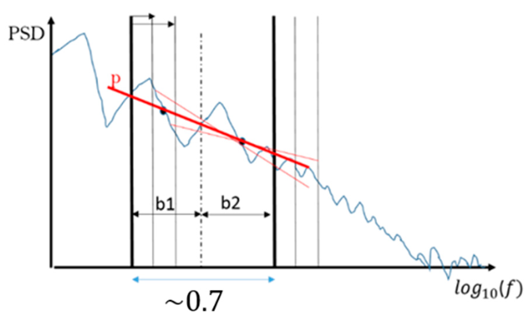
Figure 1. Schematic of the procedure used for estimating the spectral slopes in 39 frequency bands of constant width (~0.7 decade in l o g 10 scale) between 0.1 and 40 Hz. p is the slope of the thick red line obtained from a linear fit of the spectral domain delimited by the two thick vertical lines. The thin red lines show the linear fits for two spectral domains after shifting by 0.05 and 0.1 decade as indicated by the 2 horizontal arrows and the thin vertical lines (see text for more details).
Atmosphere 10 00384 g001
Figure 2. A “strong turbulence” case during FLT05A around 1635 m altitude. (a) A 1–D streamwise frequency spectra of U time series. Mean spectrum averaged over 10 consecutive (overlapping) time intervals (black). The corresponding non averaged spectra (gray). The blue line shows the −5/3 slope. The vertical thick dashed lines show the 0.1−40 Hz frequency range used for the analysis. (b) The corresponding time series of U highlighted in black. (c) Same as (a) for T. (d) Same as (b) for T. (e) Slopes of U (blue) and T (red) spectra vs. f m a x . The horizontal solid and dashed lines show −5/3 and −5/3 ± 0.25 slopes, respectively. (f) The corresponding estimates of ε   (blue) and C T 2 (red) vs. f m a x .
Atmosphere 10 00384 g002
Figure 3. The same as Figure 2 for a “Weak turbulence” case during FLT15D around 3321 m altitude.
Atmosphere 10 00384 g003
Figure 4. The same as Figure 2 for a case with strong disturbances in U spectra during FLT15A around 3526 m altitude.
Atmosphere 10 00384 g004
Figure 5. Spectral slopes of T and U spectra vs. altitude for the various frequency bands (FLT05A1). (Red): p > 5 / 3 + 0.5 (cyan), 5 / 3 0.25 < p < 5 / 3 + 0.25 , (blue): p < 5 / 3 0.5 , and the corresponding C T 2 and ε profiles after the selection criteria in black lines, when selecting 1−5 Hz (gray lines) and 5−40 Hz (gray dotted lines). The labels “N” and “A” refer to spectral bands affected by noise and artifacts, respectively (see text for more details).
Atmosphere 10 00384 g005
Figure 6. Frequency of occurrences of ranges of slopes vs. f m a x for T spectra (black) and U spectra (red).
Atmosphere 10 00384 g006
Figure 7. Histograms of l o g 10 ( γ ) for data collected during ShUREX 2016 and ShUREX 2017 without convective boundary layers (CBL), mid-level cloud base (MCT) and clouds (brown) and with all data (cyan). The symbol < > refers to the mean value, “Me” to the median value and σ to the standard deviation.
Atmosphere 10 00384 g007
Figure 8. (a) Scatter plot of l o g 10 ( ε ) vs. l o g 10 ( ε C T 2 ) estimated from C T 2 using Equation (6) and < l o g 10 ( γ ) > = 0.28   with measured N 2 (brown) and with N 2 = 1.47   10 4   rad 2 s 2 (blue). Thick dashed and solid lines show the corresponding regression lines. (b) Histogram of mixing efficient coefficient χ m . The vertical dashed line shows χ m = 0.2 (c) Histogram of flux Richardson number R f . The vertical dashed line shows R f = 0.17 .
Atmosphere 10 00384 g008
Figure 9. Vertical profiles of (a) C T 2 (blue) and ε (black), (b) ε (black), ε C T 2 (blue) and N 2 (red), (c) K θ (black) and K θ ( C T 2 ) (blue), (d) L O (black) and L O ( C T 2 ) (blue), for FLT05A1. The gray shaded areas show the CBL depth. “T1” refers to a turbulent layer discussed in the text.
Atmosphere 10 00384 g009
Figure 10. The same as Figure 9 for FLT28A1. The gray shaded areas show the CBL depth.
Atmosphere 10 00384 g010
Figure 11. The same as Figure 9 for FLT40A1. Here, the gray shaded areas does not show CBL range but the height range where air was cloudy (saturated). “T2” refers to a turbulent layer discussed in the text.
Atmosphere 10 00384 g011
Figure 12. (a) Histogram of eddy diffusivity l o g 10 ( K θ   ( m 2 s 1 ) ) with measured N 2 (gray) and with N 2 = 1.47   10 4   rad 2 s 2 (black). The solid and dashed horizontal segments are the observed ranges of values after Alisse and Sidi [29] and Bertin et al. [44] from high resolution balloon measurements for stratospheric heights. (b) Same as (a) for l o g 10 ( L O   ( m ) ) .
Atmosphere 10 00384 g012
Figure 13. (a) Histograms of l o g 10 ( L O ) (black) and l o g 10 ( L O ( C T 2 ) ) (gray). (b) Scatter plot of l o g 10 ( L O ) vs. l o g 10 ( L O ( C T 2 ) ) . The red line is a regression line.
Atmosphere 10 00384 g013
Figure 14. Histogram of l o g 10 ( R e b ) .
Atmosphere 10 00384 g014
Figure 15. (a) Vertical profile of horizontal wind shear S = ( ( d u / d z ) 2 + ( d v / d z ) 2 ) 1 / 2 where u and v are the zonal and meridional wind components measured by V06. (b) Vertical profiles of N 2 derived from V06 (black) and FLT28A1 (red). (c) Vertical profiles of dry Ri derived from V06. The vertical gray and dashed black lines show the values of 0.25 and 1, respectively. (d) Vertical profiles of ε (black) and ε C T 2 (blue). The balloon-derived profiles were calculated at a vertical resolution of 20 m.
Atmosphere 10 00384 g015
Figure 16. The same as Figure 15 for V09 and FLT40A1.
Atmosphere 10 00384 g016
Figure 17. Vertical profiles of C T 2   (black) and N 2   (gray) obtained from FLT05D1 in the height range 1800–3500 m. The labels A, B and C refer to C T 2   and N 2 peaks discussed in the text. < N 2 > = 1.47 × 10 4   rad 2 s 2 ) is shown by the vertical dashed line.
Atmosphere 10 00384 g017
Figure 18. Histogram of difference of altitudes between selected peaks of N 2 and C T 2 .
Atmosphere 10 00384 g018
Figure 19. (a) Expanded view of Figure 15, including ε and ε C T 2 with measured and constant N 2 and L O . (b) The corresponding potential temperature profile.
Atmosphere 10 00384 g019