Weather Based Strawberry Yield Forecasts at Field Scale Using Statistical and Machine Learning Models

Abstract

Strawberry is a high value and labor-intensive specialty crop in California. The three major fruit production areas on the Central Coast complement each other in producing fruits almost throughout the year. Forecasting strawberry yield with some lead time can help growers plan for required and often limited human resources and aid in making strategic business decisions. The objectives of this paper were to investigate the correlation among various weather parameters related with strawberry yield at the field level and to evaluate yield forecasts using the predictive principal component regression (PPCR) and two machine-learning techniques: (a) a single layer neural network (NN) and (b) generic random forest (RF). The meteorological parameters were a combination of the sensor data measured in the strawberry field, meteorological data obtained from the nearest weather station, and calculated agroclimatic indices such as chill hours. The correlation analysis showed that all of the parameters were significantly correlated with strawberry yield and provided the potential to develop weekly yield forecast models. In general, the machine learning technique showed better skills in predicting strawberry yields when compared to the principal component regression. More specifically, the NN provided the most skills in forecasting strawberry yield. While observations of one growing season are capable of forecasting crop yield with reasonable skills, more efforts are needed to validate this approach in various fields in the region.

1. Introduction

Strawberries (Fragaria x ananassa) are a small fruit crop and a very high cash value crop that is grown worldwide throughout the year [1]. California is a leading agricultural producer of the United States with more than 80% of the fresh market and processed strawberries produced in the state on about half of the strawberry acreage of the nation [2,3]. Currently, fresh market and processed strawberries are worth $3.1 billion and one of the top ten most valued commodities for the state and nation’s economy [4]. Since 1990, strawberry acreage has approximately doubled [5], with 33,838 acres of strawberries planted in 2018 [6] and is projected to increase due to high value and favorable conditions. The unique coastal environment of the state offers optimum growing conditions for strawberries as western ocean exposure provides moderate temperatures year-round with warm sunny days and cool foggy nights [7].

Although the highly variable and changing climate in California can greatly influence agricultural production [8], strawberries have adapted to extremely different environmental conditions [9] and the Mediterranean climate on California’s central coast provides ideal weather conditions for strawberry fruit production. However, variability in weather patterns can influence the variability in strawberry fruit production, which can ultimately impact the market value [3,10]. Among the several studies that have been conducted to elucidate the influence of weather on strawberries, some studies have revealed how strawberry yield was significantly correlated with solar radiation [1,11,12]. While these studies also investigated the importance of solar radiation in strawberry growth and development overall, wind is also reported to be a crucial parameter that impacts the growth and yield of crops [13,14,15].

It is evident from published studies that weather exhibits significant correlations with a strawberry yield that allows us to forecast crop yields prior to harvest [16]. Along with the advancement of computational capability, the current practice has incredibly evolved with model-based discussion support systems that substantially contribute to increasing the usability of research at the field scale [17]. Moreover, integrated weather–crop modeling supports risk management in agriculture [18]. These studies suggest that the accurate collection and analysis of weather data from the nearest weather station could provide an avenue for the accurate forecast of seasonal yield and provide useful information for growers’ strategic decisions.

Under situations of high data sparsity and environmental variability, data from different measurement platforms are essential to integrate in order to translate weather and climate forecasts into forecasts of production impacts and underlying environmental and genetic factors introduce crop yield as a complex attribute prior to actual harvest [17,19,20,21]. Together with the advancement of computational power, various forms of crop simulation models have been proposed to represent crop growth, development, and yield as simulations through mathematical equations as functions of soil conditions, weather, and management practices [22].

In the past, regression methods and correlation analysis were often employed to predict strawberry yield using weather information [23]. Instead of employing environmental parameters, a different combination of energy input was successfully employed in the adaptive neuro-fuzzy inference system to forecast greenhouse strawberry yield [24]. Among the various statistical models [20], simpler versions are based on statistical information related to weather and historical yield data. Most of the previous attempts have made use of meteorological parameters to predict strawberry yield for a longer period and many sites building principal components [3,16,25].

Together with “big data” technologies and high-performance computing, machine learning techniques offer new opportunities to unravel, quantify, and understand data-intensive processes in agricultural operational environments [26,27]. For that matter, machine learning is becoming a popular tool for developing a decision support system in agriculture [28]. For instance, the artificial neural network has been applied as a non-linear modeling technique in order to quantify yield response to soil variables [29,30,31,32,33]. The literature shows that random forest has been widely used as a classification tool for predicting ecosystem or crop productivity [34,35,36]. Moreover, limited studies have explored the prediction capabilities using random forest. With regard to strawberries, very few machine-learning models have been developed to predict strawberry yield [32,37]. There is a lack of robust and integrated models that couple both field measurements and environmental parameters to make short-term predictions at the field scale using a lower amount of information.

Most of the past studies have concentrated on strawberry yield forecasts using meteorological information at the regional scale. To the best of our knowledge, there is a lack of evaluation of the various forecasting methods including machine-learning approaches for strawberries at the field scale that can benefit growers in making decisions in the peer-reviewed literature. The objectives of this paper were to investigate the correlation among various weather parameters related with strawberry yield at the field level and to evaluate yield forecasts using the predictive principal component regression (PPCR) and two machine-learning techniques: (a) a single layer neural network (NN) and (b) generic random forest (RF).

The structure of the rest of the paper is as follows. Section 2 describes the study area, data collection in the field, and the dataset obtained from the weather station. This section also describes in detail three predictive modeling approaches used in this study as well as the statistics used to assess the performance of those models. Section 3 presents the key results and relevant discussions on the interactions of input variables with strawberry yield as well as the performance of the models in predicting strawberry yield. Section 4 shows the main conclusions of this study and potential future research directions.

2. Materials and Methods

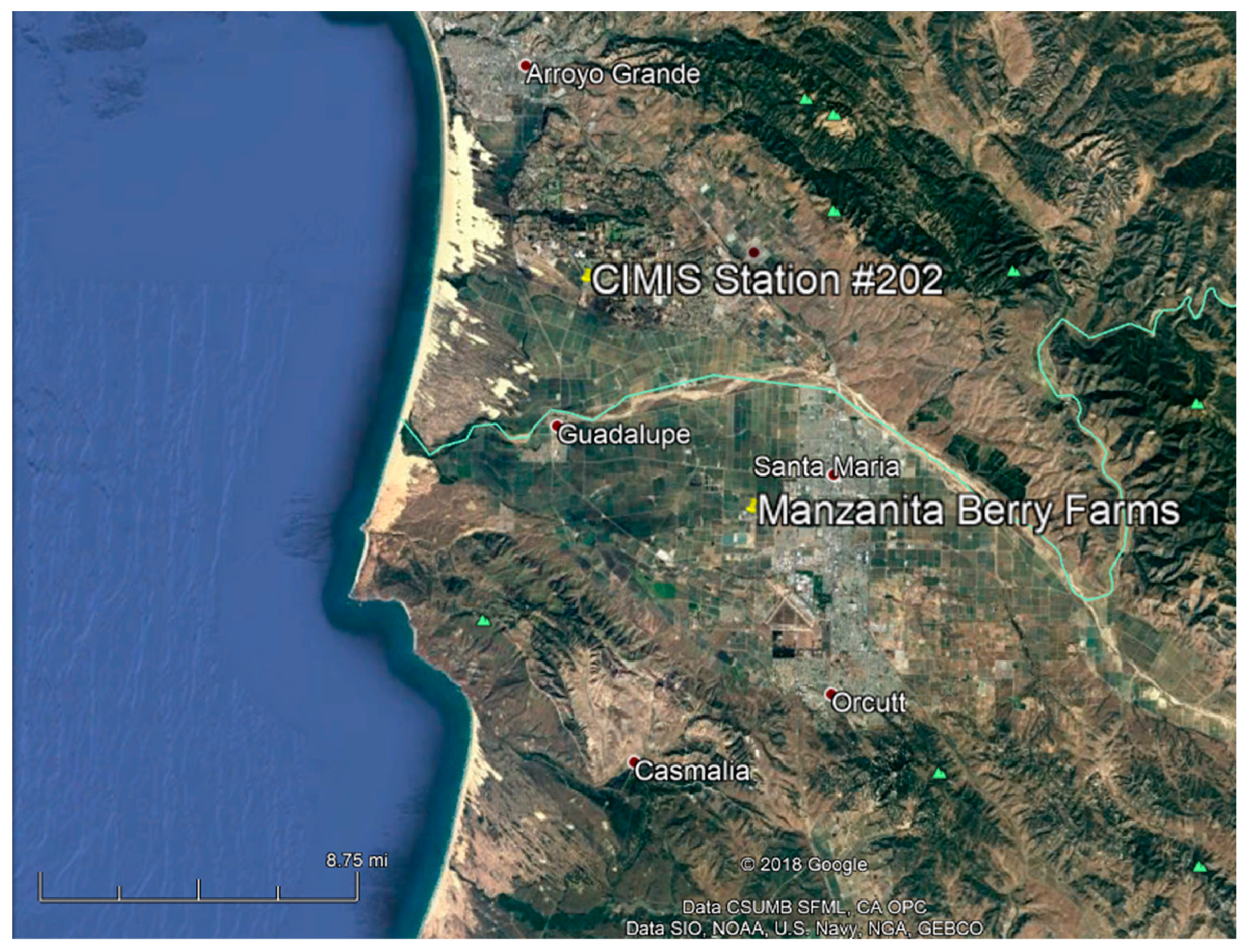
2.1. Study Area

This study was conducted on a conventional strawberry field at Manzanita Berry Farms (Figure 1) in Santa Maria (34.94, −120.48). Strawberries were transplanted into the grower’s fields in October 2018 in raised beds covered with plastic mulch. The plastic mulch protects berries from being in contact with soil, conserves water, and reduces weed infestation. Each bed was 330’ long and 5.7’ wide. A 15’-long area was marked as a sampling plot in the middle of each half of the bed. Strawberries were harvested manually from 2 February to 22 June 2018 on 36 dates.

2.2. Field Measurement Sensors

At the beginning of 2018, a leaf wetness sensor (LWS), PHYTOS 31, manufactured by Decagon Devices [38] was installed in the strawberry field. The PHYTOS 31 measures both the onset and duration of wetness on a simulated leaf, which in turn predicts the occurrence of diseases or infections, which indirectly relates to yield. The PHYTOS 31 uses capacitance technology and can sense sub-milligram levels of water condensing on the surface including frost and ice formation, thus giving a precise indication of when the sensor is wet as well as how much water is present. The sensor’s operating temperature range is between −40 °C to +60 °C. According to [39], the PHYTOS 31 does not need to be painted before use, thus eliminating the need for individual sensor calibration. Following the work of Kim et al. [40], site-specific leaf wetness duration (LWD) was computed when the LWM (leaf wetness minutes) was detected for ≥30 min in an hour. While leaf wetness minutes refers to how long free water is available on the crop surface, leaf wetness duration refers to the duration of periods when free water is present on the crop surface [41]. These indices are useful to investigate the risk of epidemics of many foliar diseases and are crucial input to many disease-warning systems.

Soil moisture and soil temperature were measured by the meter group sensor 5TM. According to Meter Environment [42], the 5TM determines volumetric water content by measuring the dielectric constant of the soil using capacitance/frequency domain technology. The soil temperature is measured by an onboard thermistor. The sensor uses a 70 MHz frequency, which minimizes salinity and textural effects, thus making the 5TM accurate in most soils and soilless media.

Ambient temperature was measured by the ECT air temperature sensor placed in a radiation shield and stacked in the field at roughly three feet in height. The ECT temperature sensor was also attached to the leaf under the canopy to measure the canopy air temperature. The chill component was introduced as it directly relates to strawberry growth and vigor. The daily and cumulative chill hours were computed by employing ambient temperature as described in [43].

All sensors were was connected to an EM50G datalogger [44] to collect hourly data for eight attributes: (a) two wetness count s(LWC1 and LWC2), (b) two wetness minutes (LWM1 and LWM2), (c) one ambient temperature (ECT1), (d) one canopy temperature (ECT2), (e) soil temperature (SMTa), and (f) volumetric moisture (SM). The actual data collection was started from February 18, 2018 until June 26, 2018 [45].

2.3. Strawberry Yield Data

Strawberry yield data from the Manzanita Berry Farms, Santa Maria Valley, California was obtained every three to four days starting from February 2, 2018 to June 22, 2018 and contained a total of 36 data points, entailing information about the total weight and aggregated weight in grams. Fruits were harvested from the sampling plots following the grower’s harvest schedule, and marketable and unmarketable berries were counted and weighed separately. Based on the daily yield data, the weekly yield information was obtained by the interpolation method used in the literature [46,47]. The aggregated seven days yield data were used for this study.

2.4. Meteorological Data

Meteorological data not collected in the field were obtained from the nearest weather station (Station 202, see Figure 1) through the network of the California Irrigation Management Information System [48]. Specifically, the parameters of net radiation (${\mathrm{R}}_{\mathrm{n}}$), solar radiation (${\mathrm{R}}_{\mathrm{s}}$), average relative humidity (${\mathrm{RH}}_{\mathrm{m}}$), dew point temperature ($\mathrm{dP}$), average vapor pressure (${\mathrm{e}}_{\mathrm{m}}$), reference evapotranspiration (${\mathrm{ET}}_{\mathrm{o}}$), the Penman-Montieth evapotranspiration (${\mathrm{PMET}}_{\mathrm{o}}$), and average wind speed ($\mathrm{ubar}$) were used in this study.

Strawberries are transplanted in the fall season, and plants start producing fruits from late spring to the end of summer. Although fruits start coming from late spring, weather influence during the fall has a carryover effect on yield. To evaluate these lagged effects of weather, the meteorological parameters from the previous fall season were gathered from the CIMIS station and converted into a weekly scale as described above. All lagged parameters with the subscript “.F” refer to the last fall and this lagged relationship was also evaluated.

2.5. Statistical Analysis

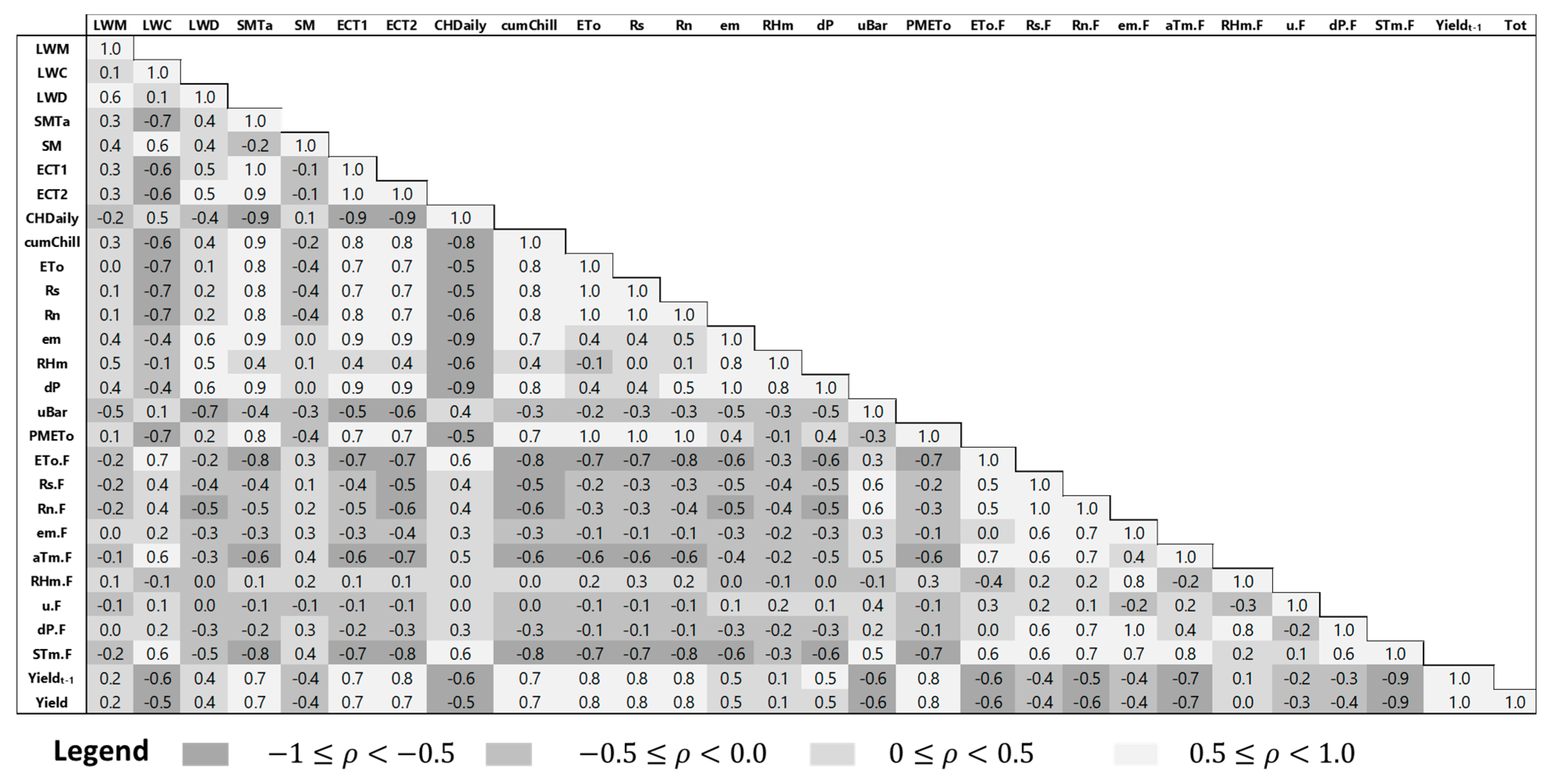
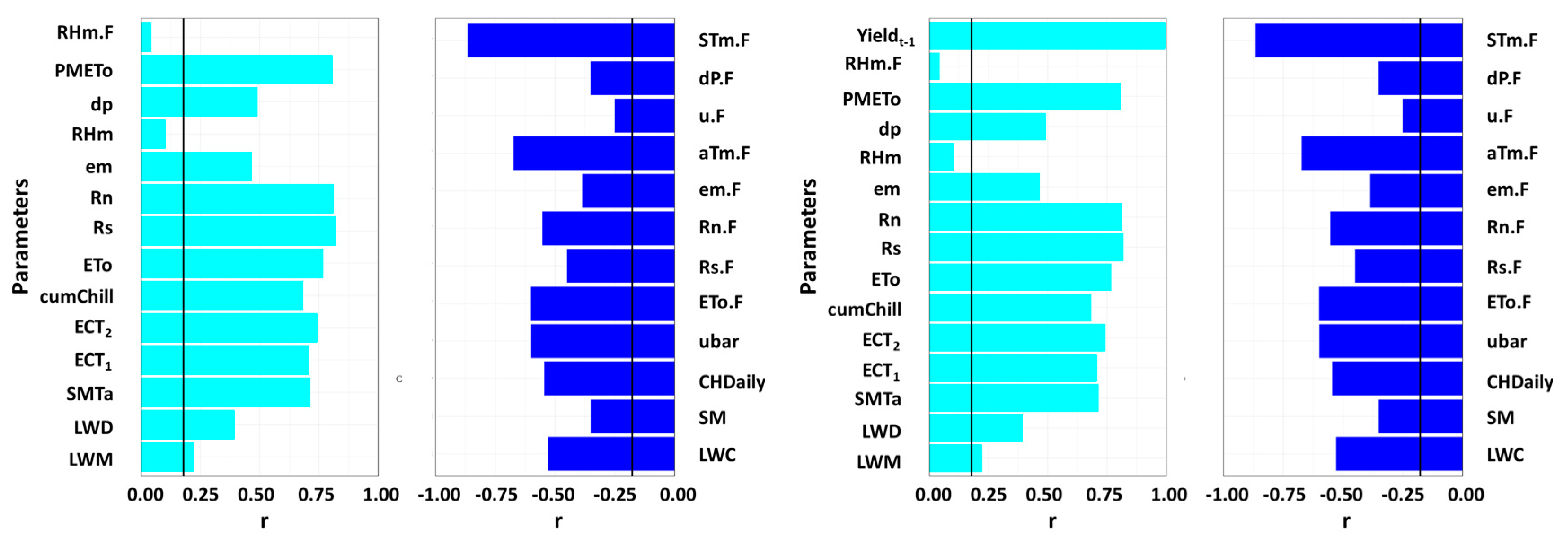
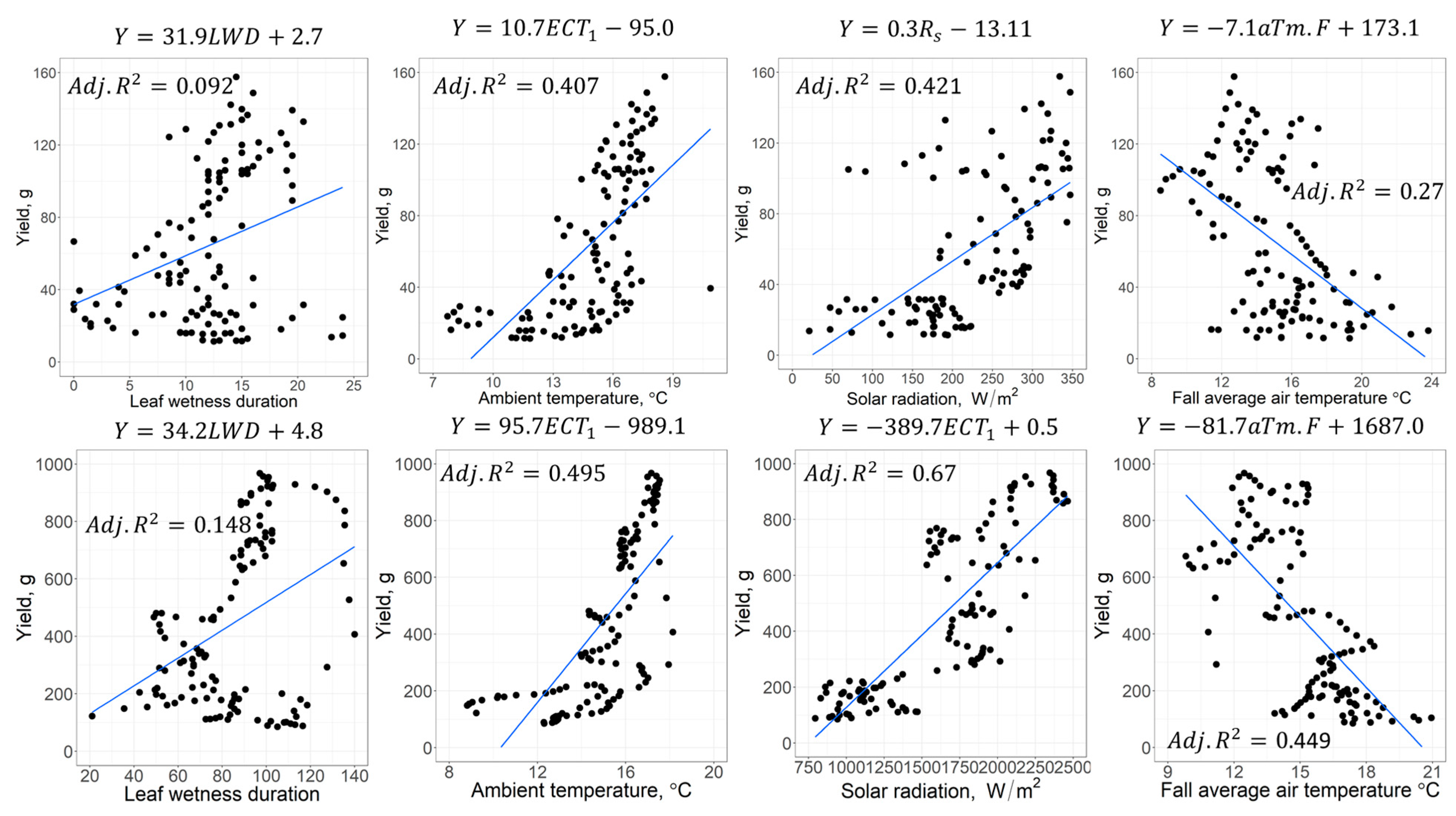
2.5.1. Correlation and Regression Analysis

Linear independence between the weather parameters and strawberry yield was tested using the Pearson product-moment correlation [49] for all parameters measured in the field and derived from the weather station. In this study, a correlation test was performed not only with yield, but also among the parameters in all time scales (hourly, daily, and weekly aggregated scale) in order to understand the influence of each variable among themselves. The significance level of each correlation test, both positive and negative, were assessed through the Student’s t-test. Furthermore, independent linear models for each variable were developed to see how each variable linearly related to the strawberry yield. The goodness of each model was reported as adjusted $R^2$.

2.5.2. Principal Component Analysis

Regression analysis is often used for predictive modeling and problem-solving purposes [27,50]. However, when the variables used in the regression are highly correlated, the issue of multicollinearity arises and violates the rule of variable independency [51]. To avoid this issue, principal component analysis was performed on all 27 parameters and used principal components to build a predictive regression model. By doing so, we could avoid the multicollinearity issue without compromising the information of the independent variables used in this study. The selection of principal components for predictive regression is a subjective choice. The idea is to retain the least principal components without compromising the information of the input variables. A wide range of the literature suggests using an arbitrary threshold value of the cumulative proportion of variance explained by the principal components to make the selection of principal components for the regression. It is a subjective tradeoff between reducing the number of principal components and the amount of variance explained by the selected principal components. In this study, we selected the principal components that explained the cumulative proportion of 90%. The resulting principal component regression equation accounting for 90% variance can be described by:

$$Y_t={\displaystyle \sum }_{i=1}^n{\alpha }_i{X}_t^i+\beta$$

(1)

where subscript $t$ refers to time and the superscript refers to the individual parameter; $Y_t$ is the crop yield at time $t$; $n$ is the number of parameters; ${\alpha }^i$ is regression coefficient or slope related to parameter $i$; $X_t^i$ is the $i^{th}$ principal component of 27 predictors at time $t$; and $\beta$ is an intercept. The principal component regression was performed in R [52]. The performance of the principal component-based regression model was evaluated in terms of the adjusted $R^2$ value.

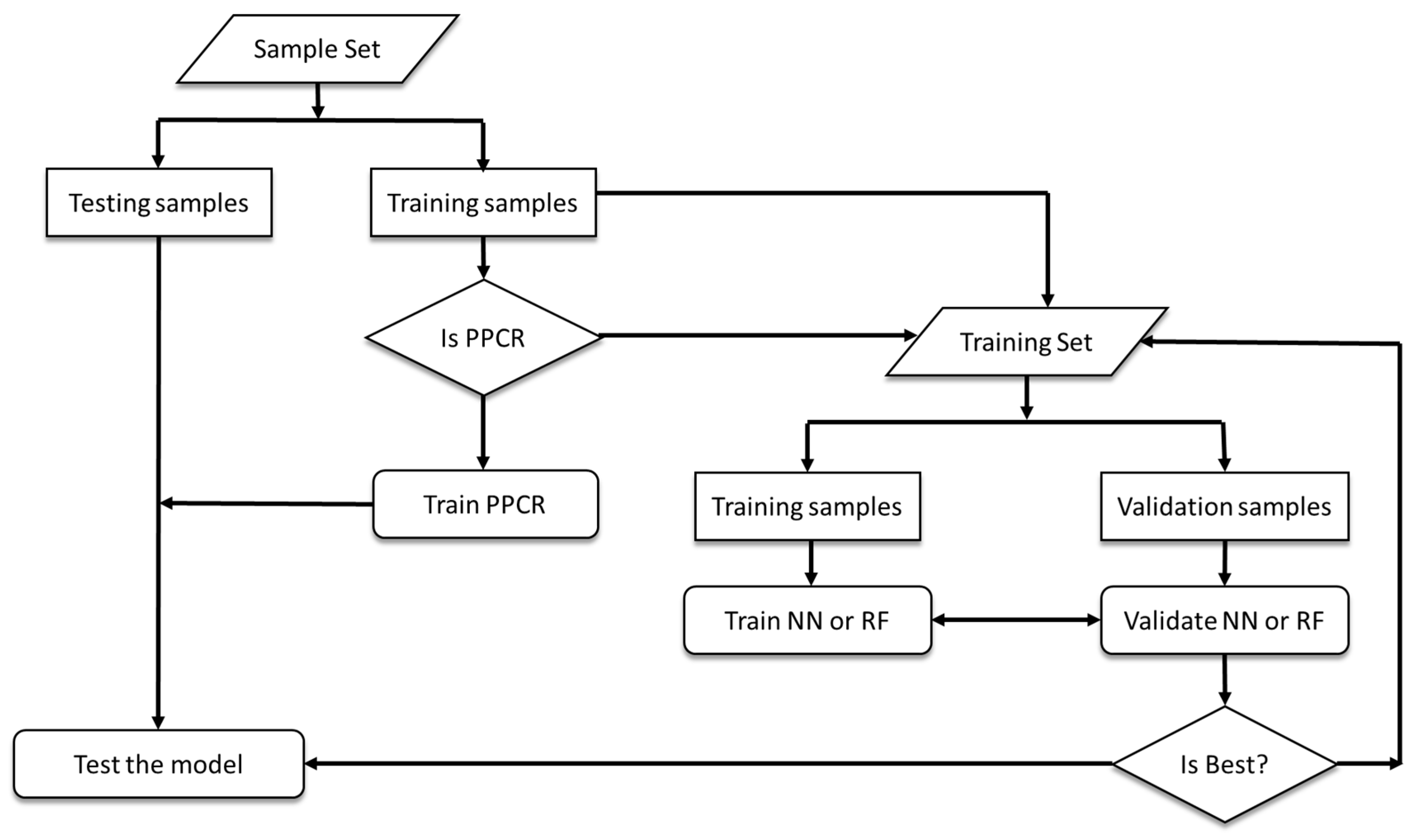
2.6. Predictive Models

This subsection primarily overviews the three kinds of predictive models and their inherent parameters. These models included the predictive principal component regression (PPCR) model, the single layer neural network (NN), and random forest (RF). Treating both the measured and weather (current and lagged) parameters as independent variables, the predictive models listed above were developed to issue weekly forecasts of strawberry yields as shown in Figure 2. Furthermore, the strategies for evaluating their performance were also explored. While the goal of this paper was to forecast strawberry yields one week ahead, all of these three predictive models were developed for a 7-day aggregated scale with the yield as a response variable accounting for all 27 input variables.

2.6.1. Predictive Principal Component Regression (PPCR)

As explained above, principal components that explained more than 90% of variability among the parameters were used to regress against the strawberry yield through the following equation:

$${\widehat{Y}}_{t+1}={\displaystyle \sum }_{i=1}^n{\alpha }_i{X}_t^i+\beta$$

(2)

where all the notations were the same as in Equation (1), except that $Y$ becomes $\widehat{Y}$ and subscript $t$ on the left side becomes $t+1$, implying that crop yield is predicted one-time step (week) ahead. The PPCR was built on 114 data points and tested on seven test points employing Equation (2).

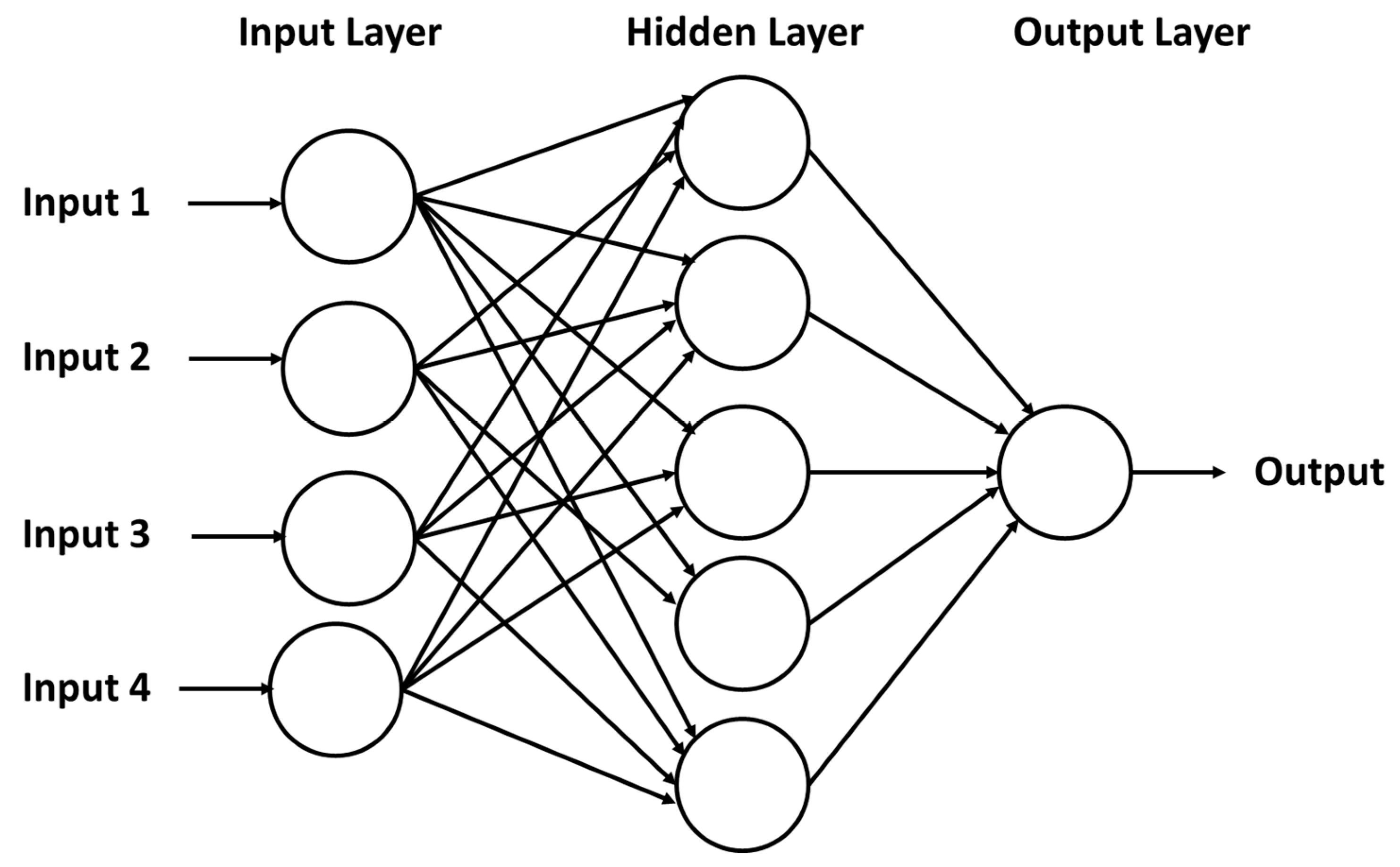
2.6.2. Neural Network (NN)

Often, the relationship between the predictor and input variables is non-linear. The neural network offers solutions to these complex non-linear relationships to explain the variability of crop productions [53]. Several successful applications of the NN for yield prediction have been reported in the literature [32,51,52].

In this study, a neural network was developed by using the input variables discussed in the previous section and employing resilient backpropagation. This approach allows for flexible settings through the custom-choice of error and the activation function to train feed-forward neural networks [54]. For example, this function provides the opportunity to define the required number of hidden layers and hidden neurons according to the needed complexity [55]. As illustrated in Figure 3, a feed-forward multi-layer perceptron neural network (NN) comprises generically three layers: (a) the input, (b) hidden, and (c) output layer and can mathematically be expressed as:

$$Y=f\left({\mathit{W}}^T\mathit{X}+b\right)$$

(3)

where $Y$ denotes the response variable; $\mathit{X}$ is the vector of input variables; $\mathit{W}$ is the set of synaptic weights; and $b$ is the bias [56].

The NN parameters included a number of hidden nodes, learning rate, activation function, and initialization of synaptic weights. These parameters were systematically chosen in this study in order to obtain the optimum NN model. The number of neurons (nodes) in the hidden layer was kept at half of the total input variables plus a response variable. This has been a widely utilized approach in the NN [58]. Due to the number of input parameters, the hidden layer was kept to one as suggested by the literature [59]. By keeping only one hidden layer, we could avoid accumulating errors and have direct connections between the input and output layers [59]. The learning rate was varied between 0.001 and 0.2 and selected the one that resulted in the least error. As suggested by Glorot and Bengio [60], Xavier’s random weight initialization scheme was selected for synaptic weights and varied randomly between $-1/\surd n$ and $1/\surd n$, where $n$ is the number of the input parameters, i.e., $n=27$ in this study. Three types of activation functions: (a) logistic, (b) hyperbolic tangent, and (c) softmax [61] were used to obtain the optimum one. While training the neural network, the entire process involves an optimization process to determine the optimal synaptic weights $\mathit{W}$ to minimize the error function [53].

In most machine learning approaches, one needs to guarantee the stable convergence of the weight and biases. Normalizing all of the variables or having the same range of values for each of the inputs solves the problem of the network being ill-conditioned. In fact, normalization of the data allows us to easily deal with the attributes of different units and scales in order to converge to better results. In this study, the max–min procedure was used to normalize the data so that all of the input and output variables ranged from 0–1. To do this, each attribute was multiplied by the difference of the maximum and minimum and then adding the minimum values to it.

The 114 data points were partitioned into a training set with 70% and a validation set with 30% of the set. The training and validation datasets were randomly selected as in leave-one-out cross-validation. The goal of the cross-validation was to obtain the optimum model to be used to train the model [19]. In this study, the training and cross-validation sets were randomly sampled, with 500 set as the maximum seeds. Among them, the best neural network with the least deviation ratio, defined in Section 2.6.4 on the cross-validation set, was selected to test the unused data points.

2.6.3. Random Forest (RF)

The random forest is an ensemble of multiple decision trees, each of which depends on the values of a random vector sampled independently and with the same distribution for all trees in the forest [62]. The use of random forests has been popular in predicting a continuous response variable like a regression that fits an ensemble of decision tree models to a set of data [63]. The use of random forest (RF) has been widely recognized in the literature for crop prediction applications [34,63,64,65].

The random forest model was developed using the same set of input variables and with the inherent parameters listed in

Table 1. Inherent parameters set for the neural network (NN) and random forest (RF).

Neural Network (NN)	Random Forest (RF)
layers: 3 (input, hidden, & neurons)	mtry: varied from $9$ to 27
hidden neurons: half of the total parameters	where $n_p$ is a number of available predictors
activation function: logistic, hyperbolic tangent and softmax function error function: logistic function
algorithm: resilient backpropagation	ntree: 100 to 500 with increment in 25 trees
learning rate: 0.01	giving 17 scenarios
thresholds: 0.05
stepmax: 106
maximum seed = 500	seed: 100

. To have a good balance between area under the receiver operating characteristic curve and processing time, a random forest should have a number of trees between 64 and 128 [66]. This study initialized the RF regression models for 100 trees, which are the number of branches that will grow after each time split, and was increased by 25 up to 500. Split points were chosen from a random subset of all available predictor variables. By default, one-third of all available predictor variables are randomly collected to sample at each split time for the regression models [67,68,69]. In order to ensure the best performance, such parameters were increased up to total predictors. The process was repeated from 1 to 100 seeds in order to reflect a “random search”, which ensures proper combinations of a range of hyper-parameters as it reaches a very good combination very quickly [70]. In this way, each parameter set produced $1700\times 19$ RF models for the present set of input variables.

Similar to the NN, cross-validation was performed following the 70–30 thumb rule for 100 seeds prior to the selection of the best model as explained in Section 2.6.2 and shown in Figure 2 for 100 seeds. Random forest, being invariant to monotonic transformations of individual feature, does not show any improvement during the translation of features. Moreover, the prediction accuracy of decision tree models is invariant under any strictly monotone transformation of the individual predictor variables [71]. Therefore, all predictors were used without any normalization in contrast to the NN.

2.6.4. Performance Strategies

To compare the observed and modeled results, the adjusted $R^2$ and root means square error (RMSE) were calculated. The RMSE gives a measure of the average error between the model outputs and observations in appropriate units and a lower RMSE is always looked for in modeling purposes. In addition, simpler statistics, named the deviation (error) and EF ratio, were defined to validate the performance of each model in percentage as:

$$F_i=\frac{\left|Y_i-{\widehat{Y}}_i\right|}{Y_i}\times 100$$

(4)

where $Y_i$ is the observed data point; ${\hat{Y}}_i$ is the (modeled) predicted value; and $i$ is the index of data points, 1,2…, $\mathrm{N}$, for $\mathrm{N}$ being the sample size. While selecting the best-trained model, a cross-validated model with the least EF values were chosen to test the unused dataset. In addition, the performance of the models was visualized by plotting the predicted versus observed during all stages of modeling.

3. Results and Discussion

Table 2. Statistics of the measured attributes in the field.

Statistics	Sensor 1		Sensor 2		Temperature			Soil Moisture Content
	Count	Minutes	Count	Minutes	Ambient	Canopy	Soil
					$°\mathbf{C}$	$°\mathbf{C}$	$°\mathbf{C}$	${\mathbf{m}}^3/{\mathbf{m}}^3$
Minimum	360	0	436	0	−2	−1	6	0.11
Average	450	26	463	55	15	14	17	0.13
Maximum	961	1960	863	1998	33	30	32	0.32

includes the statistics of all of the parameters collected by the aforementioned sensors showing the range of each variable that includes the leaf wetness count and leaf wetness minutes from two sensors, the ambient, canopy, and soil temperature as well as the volumetric soil moisture in the strawberry leaf.

3.1. Statistical Analysis

Figure 4 portrays the correlations among the input parameters on a weekly scale. The input variables are highly correlated with variable patterns. Figure 5 shows that most of the parameters were significantly correlated with the hourly and weekly strawberry yield. The leaf wetness minutes (LWM) were insignificantly correlated with the yield on a daily scale, but showed significant correlation on a weekly scale. The leaf wetness duration (LWD) exhibited a higher positive correlation than the LWM, implying that the integrated version of leaf wetness may have more influence on yield. Wind speed during the current and previous fall ($ubar$ and $u.F)$ exhibited significant negative correlations, consistent with previous findings [3]. The strawberry yield showed that the strongest correlations with temperature related parameters, i.e., ambient temperature (ECT1), canopy temperature (ECT2), soil temperature (SMTa), solar radiation, and net radiation. The correlation pattern was variable with the temperature related parameters. The spring season air and soil temperature were positively correlated with yield, as opposed to the negative correlations during the last fall season.

The yield aggregated on the weekly scale showed higher correlation values for all parameters. For instance, the correlation between strawberry yield and ambient temperature (ECT1) was 0.64 on a daily scale, whereas it was 0.71 on a weekly scale. The LWM and SM had weaker and insignificant correlations on a daily scale, but on a weekly scale, they showed a significant correlation. Several variables from the previous fall and winter season showed significant correlations with strawberry yield, meaning that the weather during the early stages of strawberry growth had a significant influence on fruit production. The significant lagged parameters included net radiation, solar radiation, evapotranspiration, air temperature, and soil temperature. These results were consistent with the previous findings of strawberries and other crops in California [16,25].

The relationships between strawberry yield and weather parameters were investigated by developing 27 linear models individually for both time scales except yield at a daily scale. While Figure 6 displays four linear models of strawberry yield with dependent variables LWD, ECT1, Rs, and STm.F on the daily and weekly scales, respectively, as an example,

Table 3. The measured parameters, current, and lagged weather parameters including the adjusted $R^2$ for respective linear models.

Id	Parameters	Units	Notation	Daily	Moving Weekly
1	Average leaf wetness minutes	minutes	LWM	0.004	0.041
2	Average leaf wetness count		LWC	0.120	0.274
3	Average leaf wetness duration		LWD	0.092	0.148
4	Ambient temperature	°C	ECT1	0.460	0.505
5	Canopy temperature	°C	ECT2	0.030	0.116
6	Soil temperature	°C	SMTa	0.407	0.495
7	Volumetric soil moisture	m3/m3	SM	0.417	0.547
8	Daily chill hours	hours	CHDaily	0.189	0.292
9	Cumulated chill hours	hours	cumChill	0.431	0.462
10	Reference evapotranspiration	mm	ETo	0.338	0.585
11	Solar Radiation	Wm-2	Rs	0.421	0.667
12	Net Radiation	Wm-2	Rn	0.439	0.656
13	Average vapor pressure	kPa	em	0.134	0.210
14	Average relative humidity	%	RHm	0.000	0.002
15	Dew point	°C	dP	0.157	0.234
16	Average wind speed	ms-1	uBar	0.261	0.354
17	Penmann-Montieth Evapotranspiration	mm	PMETo	0.384	0.648
18	Fall reference evapotranspiration	mm	ETo.F	0.244	0.356
19	Fall solar radiation	Wm-2	Rs.F	0.129	0.196
20	Fall net radiation	Wm-2	Rn.F	0.242	0.300
21	Fall average vapor pressure	kPa	em.F	0.084	0.143
22	Fall average air temperature	°C	aTm.F	0.270	0.449
23	Fall average relative humidity	%	RHm.F	–0.005	–0.006
24	Fall average wind speed	ms-1	u.F	0.020	0.055
25	Fall dew point	°C	dP.F	0.071	0.116
26	Fall average soil temperature	°C	STm.F	0.739	0.748

presents the adjusted $R^2$ values of all linear models reported in Table 3.

In order to overcome multi-collinearity issues among the various parameters, all 27 parameters were utilized for the principal component analysis. The top six principal components explained more than 90% variability and were used to build a multivariate regression model to fit the observed yield data. The model fitted set had an adjusted $R^2$ value of 0.88 (Figure 7). As seen in Figure 7, the principal component-based regression model showed a modest fitting of the observed vs. predicted yield with more points scattered around the 45° lines.

3.2. Weekly Prediction of Strawberry Yield

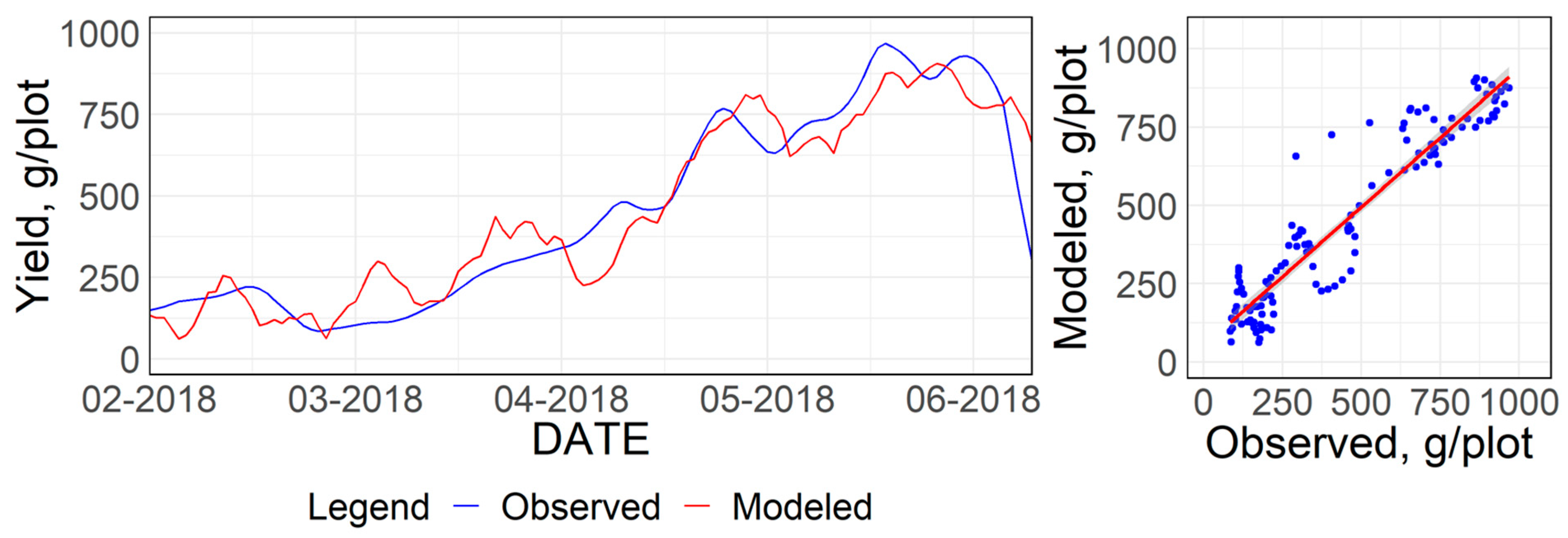
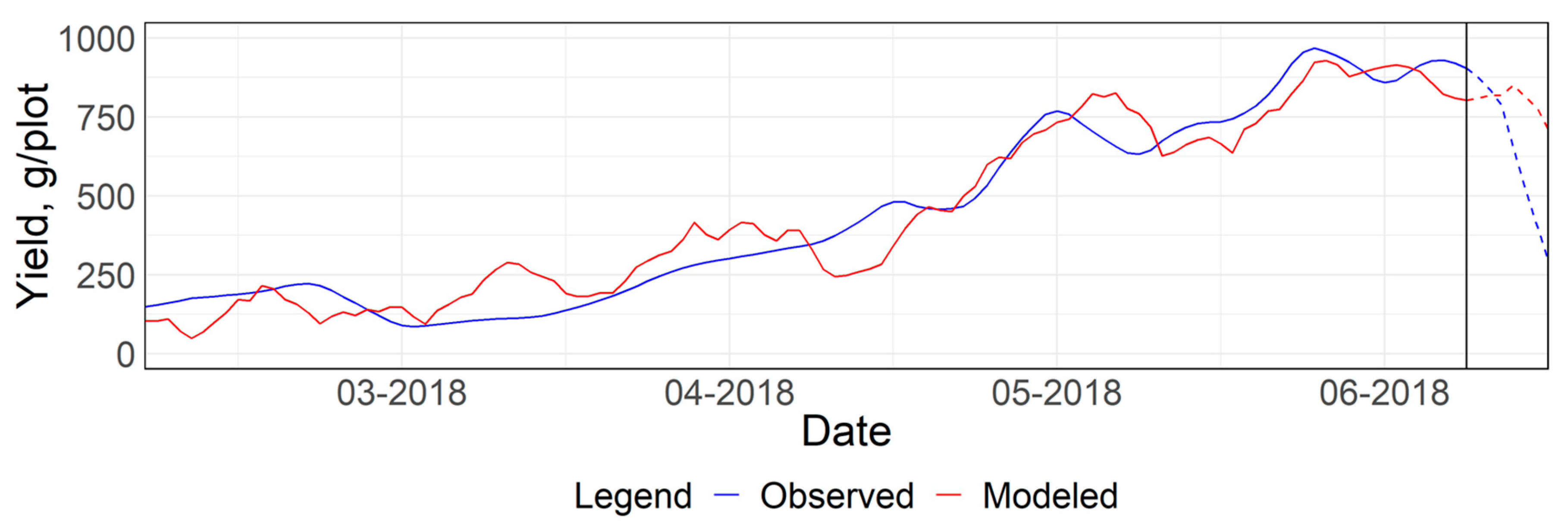
3.2.1. Predictive Principal Component Regression (PPCR)

Figure 8 shows the scatter plots of a PPCR model built using the first six principal components. The left figure shows a testing set of seven data points and the right figure shows the training set. The testing set showed poor fit with an adjusted R² of 0.42, while the training set showed an adjusted $R^2$ of 0.92.

The performance of the PPCR as shown in the right graph of Figure 8 was reflected by the close approximation of yield trends before the vertical line seen in Figure 9. Likewise, poor performance on the test set was reflected by the deviation of the red line from the blue line. The RMSE and median of EF on the training set were 81.83 g and 16.10%, respectively, and these statistics were as high as 250.90 g and 30.20%, respectively. The performance of the PPCR was not satisfactory. This could be because the derived principal components were assumed to be a linear combination of all variables and are a simplistic representation of explaining variability in yield.

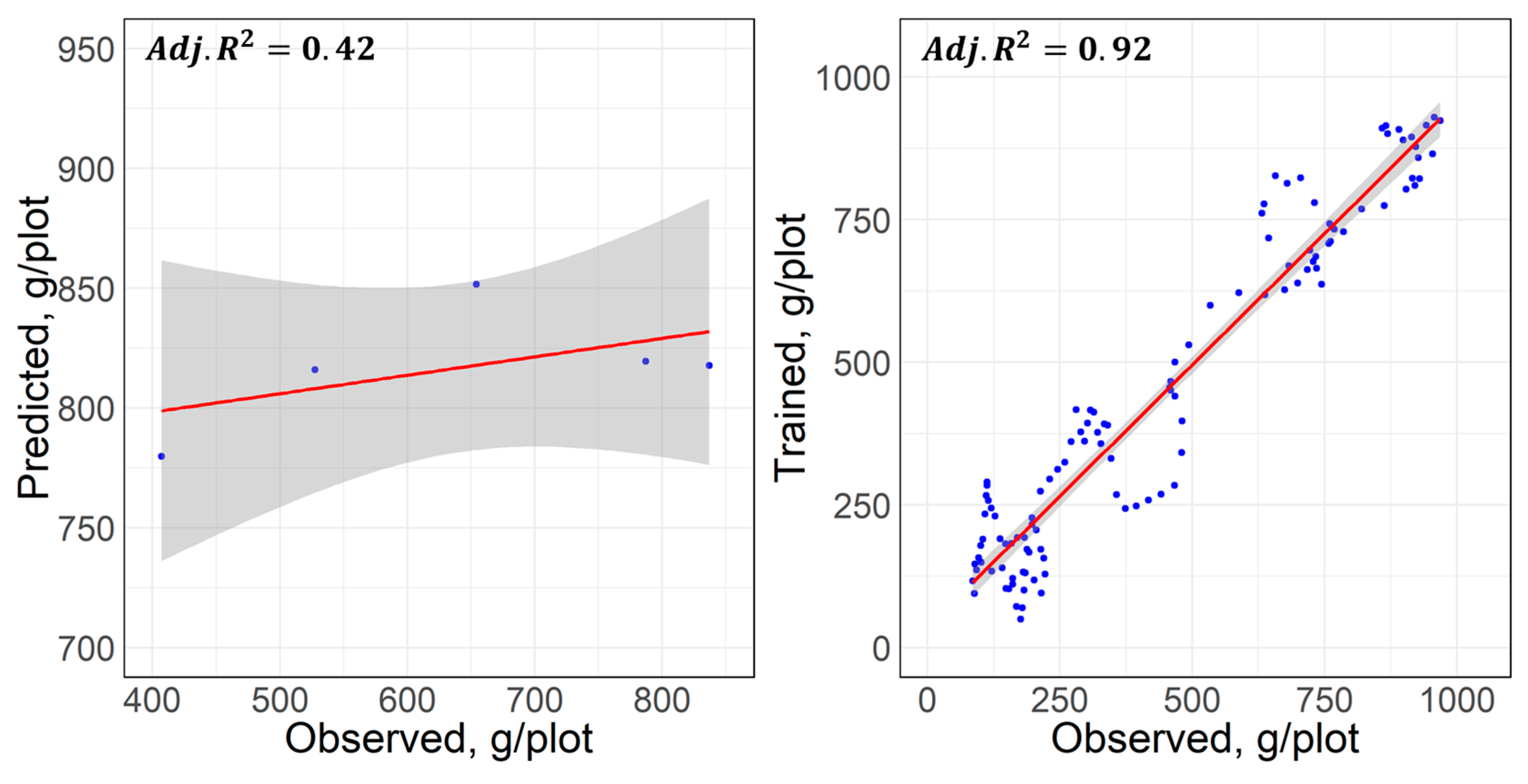
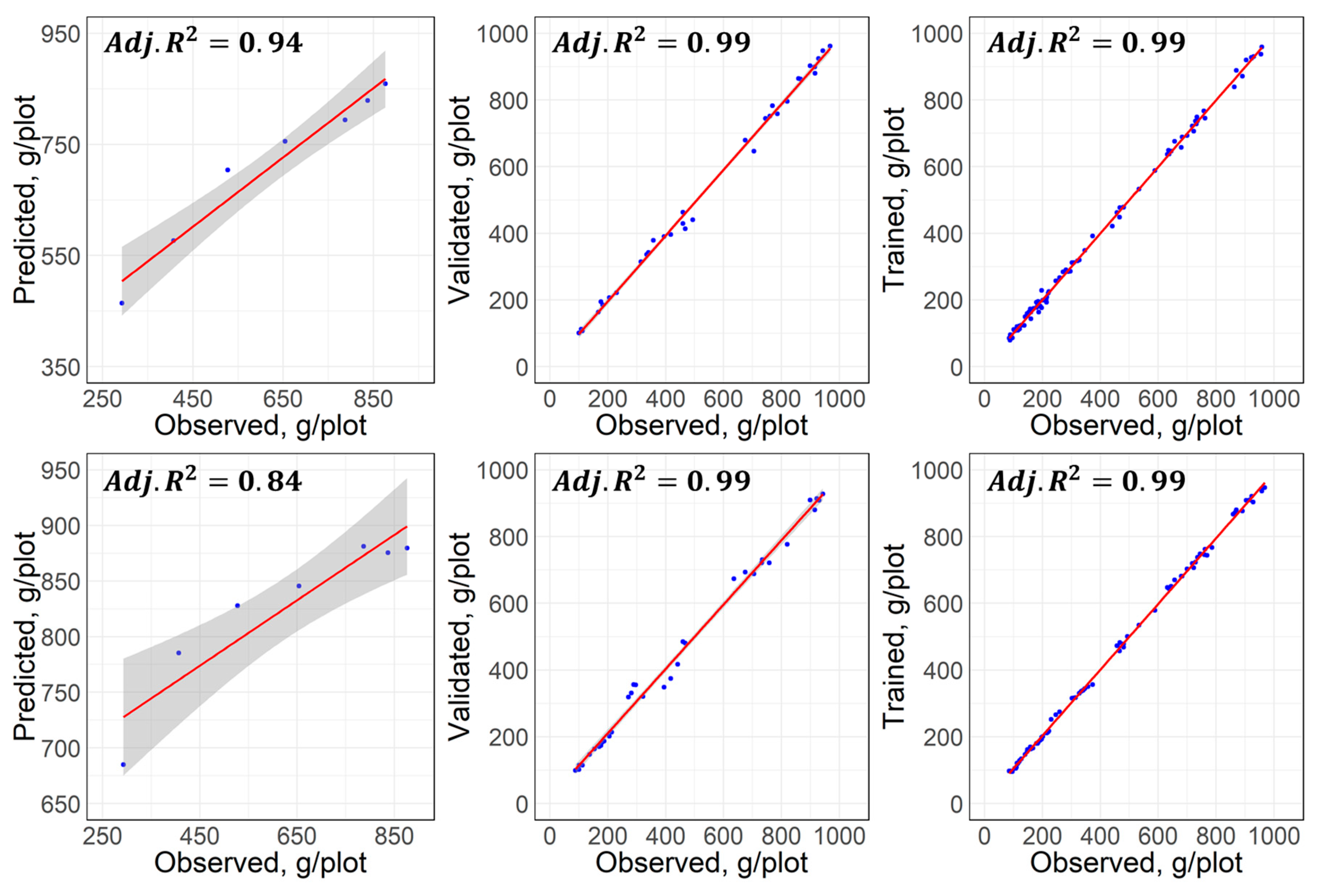
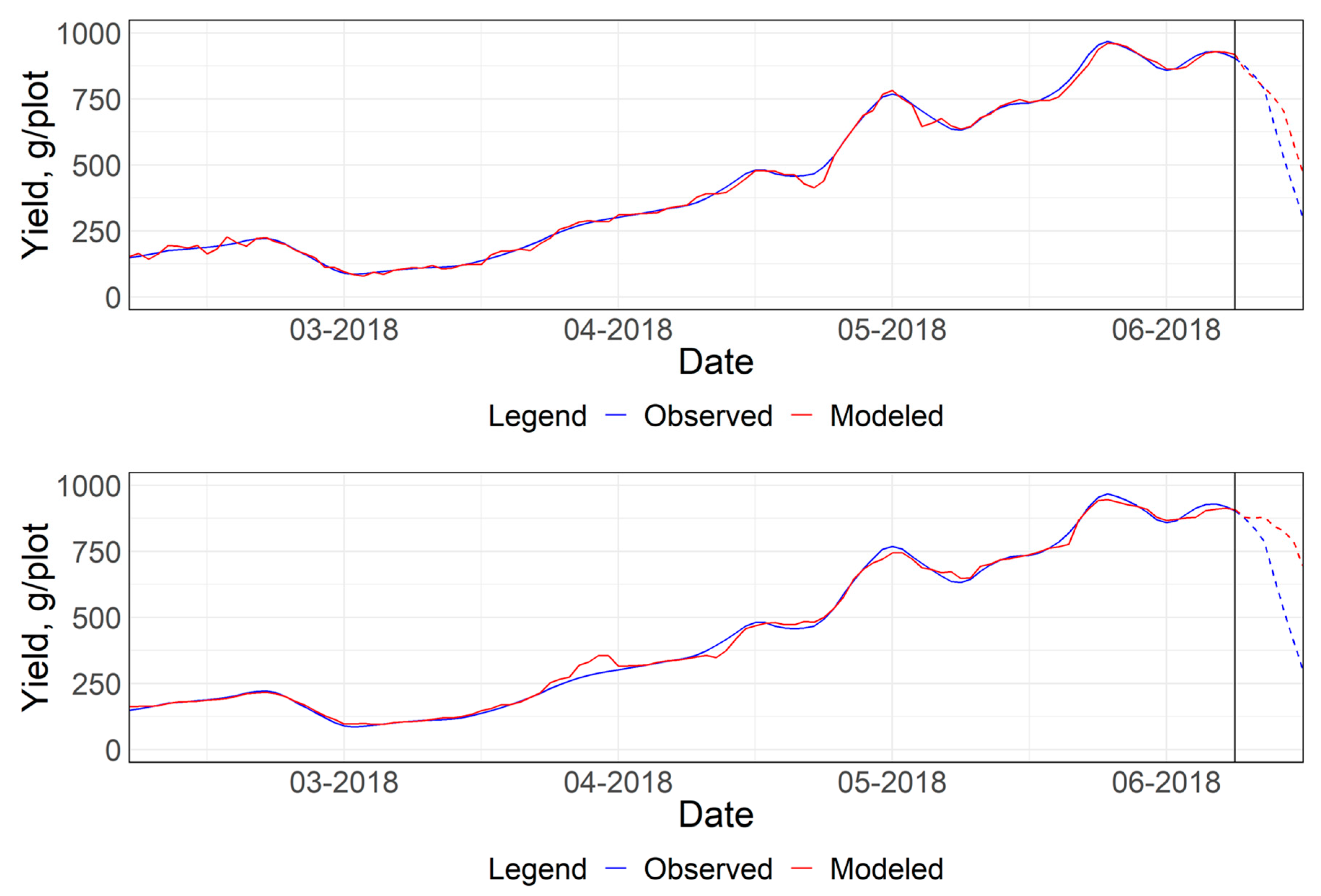
3.2.2. Machine Learning Approaches

The two machine-learning algorithms, NN and RF, were built for a similar set of parameters as described in Section 2.6.2 and Section 2.6.3. With several variations in the activation functions and learning rates, the optimal NN parameters were found for one hidden layer with the logistic function as the transfer function at a learning rate of 0.01. The maximum iterations for optimization exercise were set to 10⁶, and the error function converged within 2000 iterations. Likewise, the optimal RF model corresponded with 11 ntry and 325 trees. Figure 10 shows the modeled against the observed strawberry yield while Figure 11 shows the time series of the modeled and observed strawberry yield. It is important to note that the best model selected in both approaches corresponded to the model with the least EF values during cross-validation and was used to test the unused dataset.

Figure 10 included three scatter plots: the testing set (left), the best cross-validated set (center), and the corresponding trained model (right). The scatterplot shows that most of the points were scattered around the 1:1 line with $R^2$ values close to one during the training and validation stage, referring to a much better performance when compared to the PPCR (Figure 8). The better performance of the cross-validated model was also reflected in the better prediction skills as observed. Furthermore, the goodness of these machine-learning approaches was corroborated in the right bottom block of

Table 4. Performance of the predictive models shown in Figure 8, Figure 9, Figure 10 and Figure 11.

Data Set	Statistics	Predictive model
		PPCR	NN	RF
Training	RMSE, g	81.83	11.47	9.87
	Adjusted$R^2$	0.92	0.99	0.99
	EF, %	16.10	2.20	1.74
Validation	RMSE, g		20.85	27.49
	Adjusted$R^2$		0.99	0.99
	EF, %		1.43	2.72
Testing	RMSE, g	250.90	119.58	249.07
	Adjusted$R^2$	0.51	0.95	0.84
	EF, %	30.20	15.49	29.27

by high-adjusted $R^2$ values.

The optimum models shown in Figure 10 were represented in a time series plot of strawberry yield in Figure 11. The top plot refers to the NN and the bottom plot refers to the RF, with a vertical line that separates the testing set from the dataset that was used to build the model. The RMSE during the cross-validation was relatively low at 20.85 grams, but the RMSE during the test was higher at 119.58 grams for NN. Similarly, for RF, the RMSE during cross-validation was 27.49 grams, but 249.07 grams in testing. These statistics of both the NN and RF were associated with the least median of the EF ratios during cross-validation, which was 1.42% and 2.72%, respectively.

Based on the summary in Table 4 it is evident that the machine learning models performed much better than the statistical PPCR model in terms of the EF and RMSE. More specifically, the NN showed the least RMSE (119) and the highest adjusted R² (0.95) when compared to the PPCR (250, 0.51) and RF (249, 0.84), respectively.

4. Conclusions and Future Research

While evaluating the relationship between field measurement, meteorological attributes, and weekly strawberry yield at the Manzanita Berry Farms, most of the weather parameters showed a significant correlation with strawberry yield. These significant correlations justified the development of strawberry yield forecasting models. This study compared predictive principal component regression (PPCR), neural network (NN), and random forest (RF) strawberry yield forecasting models using field-based and nearest weather station parameters. All three approaches showed potential in forecasting strawberry yield using meteorological information, however, the machine learning approaches provided more robust forecasts when compared to the statistical approach. More specifically, the NN showed the best skills in forecasting strawberry yield at the field scale when compared to other methods. This study was based on the data collected from one strawberry growing season and the machine-learning approaches showed significant prediction skills. Future efforts are needed to collect data for more than one growing season and at various other locations to validate these models to gain confidence in making these models more operational.

References

1. Palencia, P.; Martínez, F.; Medina, J.J.; López-Medina, J. Strawberry yield efficiency and its correlation with temperature and solar radiation. Hortic. Bras. 2013, 31, 93–99. [Google Scholar] [CrossRef] [Green Version]
2. UCANR. Crop Profile for Strawberries in California. Available online: https://ucanr.edu/datastoreFiles/391-501.pdf (accessed on 1 April 2019).
3. Pathak, T.B.; Dara, S.K.; Biscaro, A. Evaluating correlations and development of meteorology based yield forecasting model for strawberry. Adv. Meteorol. 2016, 2016. [Google Scholar] [CrossRef]
4. CDFA. CDFA—Statistics. Available online: https://www.cdfa.ca.gov/statistics/ (accessed on 16 March 2019).
5. USDS/NASS. USDA/NASS 2018 State Agriculture Overview for California. Available online: https://www.nass.usda.gov/Quick_Stats/Ag_Overview/stateOverview.php?state=CALIFORNIA (accessed on 6 April 2019).
6. California Strawberry Commission. 2018 California Strawberry Acreage Survey Update; California Strawberry Commission: Watsonville, CA, USA, 2018. [Google Scholar]
7. California Strawberry Commission. FARMING—California Strawberry Commission. Available online: https://www.calstrawberry.com/Portals/2/Reports/Industry%20Reports/Industry%20Fact%20Sheets/California%20Strawberry%20Farming%20Fact%20Sheet%202018.pdf?ver=2018-03-08-115600-790 (accessed on 5 April 2019).
8. Pathak, T.; Maskey, M.; Dahlberg, J.; Kearns, F.; Bali, K.; Zaccaria, D. Climate change trends and impacts on California agriculture: A detailed review. Agronomy 2018, 8, 25. [Google Scholar] [CrossRef]
9. Rieger, M. Introduction to Fruit Crops; CRC Press: Boca Raton, FL, USA, 2006; ISBN 1-4822-9805-8. [Google Scholar]
10. Condori, B.; Fleisher, D.H.; Lewers, K.S. Relationship of strawberry yield with microclimate factors in open and covered raised-bed production. Trans. ASABE 2017, 60, 1511–1525. [Google Scholar] [CrossRef]
11. Casierra-Posada, F.; Peña-Olmos, J.E.; Ulrichs, C. Basic growth analysis in strawberry plants (Fragaria sp.) exposed to different radiation environments. Agron. Colomb. 2012, 30, 25–33. [Google Scholar]
12. Li, H.; Li, T.; Gordon, R.J.; Asiedu, S.K.; Hu, K. Strawberry plant fruiting efficiency and its correlation with solar irradiance, temperature, and reflectance water index variation. Environ. Exp. Bot. 2010, 68, 165–174. [Google Scholar] [CrossRef]
13. Waister, P. Wind as a limitation on the growth and yield of strawberries. J. Hortic. Sci. 1972, 47, 411–418. [Google Scholar] [CrossRef]
14. MacKerron, D. Wind damage to the surface of strawberry leaves. Ann. Bot. 1976, 40, 351–354. [Google Scholar] [CrossRef]
15. Grace, J. 3. Plant response to wind. Agric. Ecosyst. Environ. 1988, 22, 71–88. [Google Scholar] [CrossRef]
16. Lobell, D.; Cahill, K.; Field, C. Weather-based yield forecasts developed for 12 California crops. Calif. Agric. 2006, 60, 211–215. [Google Scholar] [CrossRef] [Green Version]
17. Hansen, J.W. Integrating seasonal climate prediction and agricultural models for insights into agricultural practice. Philos. Trans. R. Soc. B Biol. Sci. 2005, 360, 2037–2047. [Google Scholar] [CrossRef] [PubMed] [Green Version]
18. Jones, J.W.; Hansen, J.W.; Royce, F.S.; Messina, C.D. Potential benefits of climate forecasting to agriculture. Agric. Ecosyst. Environ. 2000, 82, 169–184. [Google Scholar] [CrossRef]
19. Newlands, N.K.; Zamar, D.S.; Kouadio, L.A.; Zhang, Y.; Chipanshi, A.; Potgieter, A.; Toure, S.; Hill, H.S. An integrated, probabilistic model for improved seasonal forecasting of agricultural crop yield under environmental uncertainty. Front. Environ. Sci. 2014, 2, 17. [Google Scholar] [CrossRef]
20. Basso, B.; Cammarano, D.; Carfagna, E. Review of Crop Yield Forecasting Methods and Early Warning Systems. In Proceedings of the First Meeting of the Scientific Advisory Committee of the Global Strategy to Improve Agricultural and Rural Statistics, FAO Headquarters, Rome, Italy, 18–19 July 2013; pp. 18–19. [Google Scholar]
21. Vangdal, E.; Meland, M.; Måge, F.; Døving, A. Prediction of fruit quality of plums (Prunus domestica L.). In Proceedings of the III International Symposium on Applications of Modelling as an Innovative Technology in the Agri-Food Chain, Leuven, Belgium, 29 May–2 June 2005; Volume MODEL-IT 674, pp. 613–617. [Google Scholar]
22. Hoogenboom, G.; White, J.W.; Messina, C.D. From genome to crop: Integration through simulation modeling. Field Crops Res. 2004, 90, 145–163. [Google Scholar] [CrossRef]
23. Døving, A.; Måge, F. Prediction of strawberry fruit yield. Acta Agric. Scand. 2001, 51, 35–42. [Google Scholar] [CrossRef]
24. Khoshnevisan, B.; Rafiee, S.; Mousazadeh, H. Application of multi-layer adaptive neuro-fuzzy inference system for estimation of greenhouse strawberry yield. Measurement 2014, 47, 903–910. [Google Scholar] [CrossRef]
25. Pathak, T.; Dara, S.K. Influence of Weather on Strawberry Crop and Development of a Yield Forecasting Model. Available online: https://ucanr.edu/blogs/strawberries-vegetables/index.cfm?start=13 (accessed on 26 April 2019).
26. Liakos, K.; Busato, P.; Moshou, D.; Pearson, S.; Bochtis, D. Machine learning in agriculture: A review. Sensors 2018, 18, 2674. [Google Scholar] [CrossRef]
27. Lobell, D.B.; Burke, M.B. On the use of statistical models to predict crop yield responses to climate change. Agric. For. Meteorol. 2010, 150, 1443–1452. [Google Scholar] [CrossRef]
28. Pantazi, X.E.; Moshou, D.; Alexandridis, T.; Whetton, R.; Mouazen, A.M. Wheat yield prediction using machine learning and advanced sensing techniques. Comput. Electron. Agric. 2016, 121, 57–65. [Google Scholar] [CrossRef]
29. Drummond, S.T.; Sudduth, K.A.; Joshi, A.; Birrell, S.J.; Kitchen, N.R. Statistical and neural methods for site-specific yield prediction. Trans. ASAE 2003, 46, 5. [Google Scholar] [CrossRef]
30. Fortin, J.G.; Anctil, F.; Parent, L.-É.; Bolinder, M.A. A neural network experiment on the site-specific simulation of potato tuber growth in Eastern Canada. Comput. Electron. Agric. 2010, 73, 126–132. [Google Scholar] [CrossRef]
31. Effendi, Z.; Ramli, R.; Ghani, J.A.; Rahman, M. A Back Propagation Neural Networks for Grading Jatropha curcas Fruits Maturity. Am. J. Appl. Sci. 2010, 7, 390. [Google Scholar] [CrossRef]
32. Misaghi, F.; Dayyanidardashti, S.; Mohammadi, K.; Ehsani, M. Application of Artificial Neural Network and Geostatistical Methods in Analyzing Strawberry Yield Data; American Society of Agricultural and Biological Engineers: Minneapolis, MN, USA, 2004; p. 1. [Google Scholar]
33. Liu, J.; Goering, C.; Tian, L. A neural network for setting target corn yields. Trans. ASAE 2001, 44, 705. [Google Scholar]
34. Jeong, J.H.; Resop, J.P.; Mueller, N.D.; Fleisher, D.H.; Yun, K.; Butler, E.E.; Timlin, D.J.; Shim, K.-M.; Gerber, J.S.; Reddy, V.R. Random forests for global and regional crop yield predictions. PLoS ONE 2016, 11, e0156571. [Google Scholar] [CrossRef] [PubMed]
35. Mutanga, O.; Adam, E.; Cho, M.A. High-density biomass estimation for wetland vegetation using WorldView-2 imagery and random forest regression algorithm. Int. J. Appl. Earth Obs. Geoinf. 2012, 18, 399–406. [Google Scholar] [CrossRef]
36. Fukuda, S.; Spreer, W.; Yasunaga, E.; Yuge, K.; Sardsud, V.; Müller, J. Random Forests modeling for the estimation of mango (Mangifera indica L. cv. Chok Anan) fruit yields under different irrigation regimes. Agric. Water Manag. 2013, 116, 142–150. [Google Scholar] [CrossRef]
37. Lee, M.; Monteiro, A.; Barclay, A.; Marcar, J.; Miteva-Neagu, M.; Parker, J. A framework for predicting soft-fruit yields and phenology using embedded, networked microsensors, coupled weather models and machine-learning techniques. BiorXiv 2019. [Google Scholar] [CrossRef]
38. Leaf Wetness Sensor from Decagon Devices: Campbell Update 1st. Available online: https://www.campbellsci.com/leaf-wetness-article (accessed on 7 April 2019).
39. Meter PHYTOS 31. Available online: http://library.metergroup.com/Manuals/20434_PHYTOS31_Manual_Web.pdf (accessed on 4 July 2019).
40. Kim, K.; Gleason, M.; Taylor, S. Forecasting site-specific leaf wetness duration for input to disease-warning systems. Plant Dis. 2006, 90, 650–656. [Google Scholar] [CrossRef]
41. Sentelhas, P.; Monteiro, J.; Gillespie, T. Electronic leaf wetness duration sensor: Why it should be painted. Int. J. Biometeorol. 2004, 48, 202–205. [Google Scholar] [CrossRef]
42. METER. Legacy Soil Moisture Sensors | METER. Available online: https://www.metergroup.com/environment/articles/meter-legacy-soil-moisture-sensors/ (accessed on 17 June 2019).
43. Bolda, M. Chilling Requirements in California Strawberries. Available online: https://ucanr.edu/blogs/blogcore/postdetail.cfm?postnum=722 (accessed on 30 April 2019).
44. ECH2O 5TM | Soil Moisture and Temperature Sensor | METER Environment. Available online: https://www.metergroup.com/environment/products/ech2o-5tm-soil-moisture/ (accessed on 7 April 2019).
45. California Farms California Strawberries, Strawberry Fields, Crops and Events. Available online: http://www.seecalifornia.com/farms/california-strawberries.html (accessed on 7 April 2019).
46. Snyder, R.; Spano, D.; Pawu, K. Surface renewal analysis for sensible and latent heat flux density. Bound. Layer Meteorol. 1996, 77, 249–266. [Google Scholar] [CrossRef]
47. Marino, G.; Zaccaria, D.; Snyder, R.L.; Lagos, O.; Lampinen, B.D.; Ferguson, L.; Grattan, S.R.; Little, C.; Shapiro, K.; Maskey, M.L. Actual Evapotranspiration and Tree Performance of Mature Micro-Irrigated Pistachio Orchards Grown on Saline-Sodic Soils in the San Joaquin Valley of California. Agriculture 2019, 9, 76. [Google Scholar] [CrossRef]
48. CIMIS, California Irrigation Mangagement Information System; Department of Water Resources: Sacramento, CA, USA, 1982. Available online: https://cimis.water.ca.gov/ (accessed on 7 April 2019).
49. Becker, R.; Chambers, J.; Wilks, A. The New S Language; Wadsworth & Brooks/Cole; Pacific: Wisconsin, IL, USA, 1988. [Google Scholar]
50. Sellam, V.; Poovammal, E. Prediction of crop yield using regression analysis. Indian J. Sci. Technol. 2016, 9, 1–5. [Google Scholar] [CrossRef]
51. Jackson, J.E. A User’s Guide to Principal Components; John Willey Sons Inc.: New York, NY, USA, 1991; p. 40. [Google Scholar]
52. R Core Team. R: A Language and Environment for Statistical Computing; R Foundation for Statistical Compiting: Vienna, Austria, 2018. [Google Scholar]
53. Li, A.; Liang, S.; Wang, A.; Qin, J. Estimating crop yield from multi-temporal satellite data using multivariate regression and neural network techniques. Photogramm. Eng. Remote Sens. 2007, 73, 1149–1157. [Google Scholar] [CrossRef]
54. Riedmiller, M.; Braun, H. A Direct Adaptive Method for Faster Backpropagation Learning: The Rprop Algorithm. In Proceedings of the IEEE International Conference on Neural Networks, San Francisco, CA, USA, 28 March–1 April 1993; Volume 1993, pp. 586–591. [Google Scholar]
55. Günther, F.; Fritsch, S. Neuralnet: Training of neural networks. R J. 2010, 2, 30–38. [Google Scholar] [CrossRef]
56. Mendes, C.; da Silva Magalhes, R.; Esquerre, K.; Queiroz, L.M. Artificial neural network modeling for predicting organic matter in a full-scale up-flow anaerobic sludge blanket (UASB) reactor. Environ. Model. Assess. 2015, 20, 625–635. [Google Scholar] [CrossRef]
57. Manzini, N. Single Hidden Layer Neural Network. Available online: https://www.nicolamanzini.com/single-hidden-layer-neural-network/ (accessed on 8 April 2019).
58. Chan, M.-C.; Wong, C.-C.; Lam, C.-C. Financial Time Series Forecasting by Neural Network Using Conjugate Gradient Learning Algorithm and Multiple Linear Regression Weight Initialization. In Computing in Economics and Finance; The Hong Kong Polytechnic University: Kowloon, Hong Kong, 2000; Volume 61, pp. 326–342. [Google Scholar]
59. Hayashi, Y.; Sakata, M.; Gallant, S.I. Multi-Layer Versus Single-Layer Neural Networks and An Application to Reading Hand-Stamped Characters; Springer: Dordrecht, the Netherlands, 1990; pp. 781–784. [Google Scholar]
60. Glorot, X.; Bengio, Y. Understanding the Difficulty of Training Deep Feedforward Neural Networks. In Proceedings of the thirteenth international conference on artificial intelligence and statistics, Sardinia, Italy, 13–15 May 2010; 2010; pp. 249–256. [Google Scholar]
61. Bergstra, J.; Desjardins, G.; Lamblin, P.; Bengio, Y. Quadratic Polynomials Learn Better Image Features (Technical Report 1337); Département d’Informatique et de Recherche Opérationnelle, Université de Montréal: Montréal, QC, Canada, 2009. [Google Scholar]
62. Breiman, L. Random forests. Mach. Learn. 2001, 45, 5–32. [Google Scholar] [CrossRef]
63. Everingham, Y.; Sexton, J.; Skocaj, D.; Inman-Bamber, G. Accurate prediction of sugarcane yield using a random forest algorithm. Agron. Sustain. Dev. 2016, 36, 27. [Google Scholar] [CrossRef]
64. Crane-Droesch, A. Machine learning methods for crop yield prediction and climate change impact assessment in agriculture. Environ. Res. Lett. 2018, 13, 114003. [Google Scholar] [CrossRef] [Green Version]
65. Narasimhamurthy, V.; Kumar, P. Rice Crop Yield Forecasting Using Random Forest Algorithm. Int. J. Res. Appl. Sci. Eng. Technol. IJRASET 2017, 5, 1220–1225. [Google Scholar] [CrossRef]
66. Oshiro, T.M.; Perez, P.S.; Baranauskas, J.A. How Many Trees in a Random Forest? Springer: Berlin, Germany, 2012; pp. 154–168. [Google Scholar]
67. RColorBrewer, S.; Liaw, M.A. Package ‘Randomforest’; University of California, Berkeley: Berkeley, CA, USA, 2018. [Google Scholar]
68. Khanh, P.D. Caret Practice. Available online: https://rpubs.com/phamdinhkhanh/389752 (accessed on 25 March 2019).
69. Liaw, A.; Wiener, M. Classification and regression by random forest, R News, vol. 2/3, 18–22. R News 2002, 2, 18–22. [Google Scholar]
70. Aly, M. What Is the Difference between Random Search and Grid Search for Hyperparameter Optimization?—Quora. Available online: https://www.quora.com/What-is-the-difference-between-random-search-and-grid-search-for-hyperparameter-optimization (accessed on 9 April 2019).
71. Galili, T.; Meilijson, I. Splitting matters: How monotone transformation of predictor variables may improve the predictions of decision tree models. arXiv 2016, arXiv:161104561. [Google Scholar]
Figure 1. Location map of the study map together with the CIMIS (California Irigation Managament Information System) station 202 at Nipomo.
Atmosphere 10 00378 g001
Figure 2. Flowchart showing the development of the strawberry yield model employing PPCR, NN, and RF.
Atmosphere 10 00378 g002
Figure 3. A generic neural network with a single hidden layer used in this study [57].
Atmosphere 10 00378 g003
Figure 4. A matrix of correlation among the input parameters as well as the response variable.
Atmosphere 10 00378 g004
Figure 5. Bar graphs showing the correlations between strawberry yield and other variables as listed in Table 3. The bars below the black line imply that the parameters are insignificant to crop yield. (Left) Daily scale. (Right) Weekly scale.
Atmosphere 10 00378 g005
Figure 6. Regression plots for the significant parameters on a daily scale (top) and 7-day moving window (bottom).
Atmosphere 10 00378 g006
Figure 7. Multivariate regression model on the top six principal components on a weekly scale. (Left) Time series plot of observed and regressed crop yield. (Right) Observed vs. regressed values.
Atmosphere 10 00378 g007
Figure 8. Scatter plots of the observed vs. modeled from a predictive principal component regression (PPCR) model. (Left) Performance of test. (Right) Training.
Atmosphere 10 00378 g008
Figure 9. Observed and modeled dynamics of strawberry yield implied by the PPCR model shown in Figure 8. The vertical line separates the sample from the training and testing.
Atmosphere 10 00378 g009
Figure 10. Scatter plots of the observed versus the modeled using the neural network, NN (top) entailing. (Left) Testing. (Center) Cross-validation. (Right) Training.
Atmosphere 10 00378 g010
Figure 11. Time series plots of strawberry yield overlaid by approximations from NN (top) and RF (bottom). The vertical line separates the sample from the training and testing seven data points.
Atmosphere 10 00378 g011