Abstract
Increasing urbanization impacts the local meteorology and the quality of life for residents. Urban surface characteristics and anthropogenic heat stress lead to urban heat island effects, changes in local circulations, precipitation alteration, and amendment of the local fluxes. These modifications have a direct effect on the life and health of residents. In this study, we assessed the impact of urbanization in Sofia (Bulgaria) using the Weather Research and Forecasting (WRF) model at 500 m resolution for the summer period of 2016. We utilized the CORINE (coordination of information on the environment) 2012 land cover database to represent the urban areas in four detailed land cover types, i.e., high-intensity residential areas, low-intensity residential areas, medium/industrial areas, and developed open spaces. We performed two experiments; in the first, we substituted an urban area with the most representative rural land cover to delineate the current impact of urbanization, while in the second, we replaced the existing built-up area (all four categories) with a hypothetical scenario of high-density residential land cover showing aggressive urban development. These experiments addressed the impact of land use changes as well as the extreme effects of ongoing high-density construction on the local meteorological conditions. The results showed that urban temperatures can increase by 5 °C and that moisture can decrease by 2 g/kg in the central part of Sofia in comparison to surrounding rural areas. The results also showed that building higher and dense urban areas can significantly increase heat flux and add additional stress to the environment.
1. Introduction
More than half of the world’s population lives in urban areas, and this proportion is expected to increase to 68% by the year 2050 [1]. The increasing urban population trend is not only common in metropolitan areas, but also in smaller urban regions. Rural populations are migrating to cities in search of better access of healthcare, education, and employment. Relatively small urban areas such as Sofia, with a population of approximately 1.25 million [2], are not exempt from these migration patterns. The problem with the lack of compulsory address registration, however, makes the city’s management believe that there are between 1.6 and 1.8 million people in the capital, approximately a quarter of the country’s population. This large-scale and relatively fast migration trend has taken its toll on the urban infrastructure, constraining resources and adversely affecting urban metabolism. Sofia faces serious challenges, including environmental degradation and increased human health risks associated with heat, noise, pollution, and crowding. This unprecedented urban population growth strengthened after Bulgaria joined the European Union, leading to increased investments and stringent new regulations. For example, many single-family houses have now been replaced with 5–7 floor buildings in residential neighborhoods, and many available open green spaces have been converted into built up and impervious areas. Attempts have been made to study the effect of urbanization in Sofia on biodiversity [3], population growth and density [4,5,6], economic, spatial and demographic trends in the urban systems [7], theoretical aspects of sustainable development of urban areas [8], and urban heat island effects [9]. To the best of our knowledge, no detailed study has evaluated the impact of urbanization on the local meteorological conditions and different scenarios of future urban development in Sofia; the importance of the aforementioned problems is the motivation for this work.
An urban environment is a mix of biotic (vegetation, animals, and humans) and the abiotic (water, land surface, wind, radiation, temperature, humidity, etc.) elements [10]. It includes remnant ecosystems (e.g., undisturbed ponds, lakes, ravines, escarpments, parks and forests), managed ecosystems (e.g., fields, tended parks, gardens, cemeteries, golf courses, and other open ground), and anthropogenic systems (e.g., roads, buildings, parking spaces, industrial and housing areas). Parks and urban forests help reduce anthropogenic heat flux and improve air quality. However, dense built-up areas and reduced green infrastructure have intensified urban heating and created hotspots throughout the city. The urban sprawl in Sofia has converted the agricultural and green city hinterlands in the valley and reached into the foothills of Vitosha and the Stara Planina mountains (Figure 1). Overall, Sofia is impacted by a significant urban heat island (UHI) effect, i.e., elevated local temperatures in urban areas compared to rural areas, especially at night, as rural/agricultural areas release heat quickly [11,12,13,14]. The UHI effects modify local meteorology, exacerbate local air pollution, reduce visibility, put stress on energy and water systems, and exacerbate morbidity [15]. Therefore, the UHI intensity (i.e., a measure of the difference between urban and surrounding rural temperature) can be as high as ~10 °C [16]. The UHI effects are pronounced during urban heat waves [17,18].
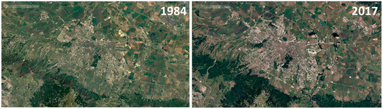
Figure 1.
Expansion in Sofia over the last few decades (1984–2017); source: images from Google Earth Pro.
Urban studies have shown that buildings and urban land use significantly modify the mesoscale flows, such as UHI effects [13,14,19], slope and valley, sea and lake breeze winds [13,20,21], and rainfall [22]. The high heat capacity of built/impervious surfaces in urban areas intensifies UHI effects by retaining daytime heat and releasing in the night [11,22]. On microscales, the local flow and thermodynamics over building blocks determine energy [23,24,25], i.e., that over street canyons turbulence and dispersion [26]. Overall, urban microscales interact with and are modified by larger scales [25,27,28]. Also, changes in urban climates provide information about the changes in the global climate [29]. Locally, there is usually a sharp contrast in energy balance, temperature, humidity, and storm runoff between urban and surrounding areas, primarily due to land use and land cover differences.
In addition to local factors, large-scale climate also has a significant impact on urban climate. For example, climate change may increase the frequency and intensity of heatwaves. Heatwaves can exacerbate UHI effects and can have detrimental impacts on urban health. Recently, the 2018 European heat wave was a period of unusually hot weather that led to record-breaking temperatures and wildfires in many parts of Europe. Recent analysis suggests that climate change has made heatwaves more than twice as likely to occur in northern Europe [30]. Bulgaria has been spared from this event, but Sofia has suffered from heat waves in previous years—the heat wave month (July 2007) was 2 °C hotter than the 2003–2013 mean in Sofia [31]; July 25th, 2009, the temperatures hit 38 °C–39 °C; July 1st, 2017 five people died, and the city’s emergency services provided assistance to around 200 people who felt unwell, as temperatures reached as high as 44 degrees Celsius [30]. Similarly, the 1995 US heat wave [32] and the 2003 European heat wave [33] led to elevated mortality rates due to the hazardous coupling of UHI effects and heat waves.
Overall, human health, energy, and resources are adversely affected by UHI effects [34,35]. At times, an increase of UHI intensity above a certain threshold can cause “regime shifts” in urban microclimates [36]. Regime shifts can occur because of interactions across social, ecological, and economic domains, and not just as the result of interactions across scales within a particular domain. Urban responses to global climate change make such shifts more likely. For example, the formation of clouds and precipitation behavior can be observed over urban areas [37,38,39].
The UHI and its impact on environment receive extensive attention in recent years especially in areas with rapid urbanization [40]. Numerical weather prediction (NWP) models are broadly used as a powerful instrument in assessment and prediction of urban effects on the environment and also help in developing adaptation and mitigation strategies [40,41,42,43]. It is worth noting the various human thermal comfort indices, e.g., Physiological Equivalent Temperature (PET) [44], Heat Stress Index (HIS) [45], Wet Bulb Globe Temperature (WBGT) [46], Universal Thermal Climate Index (UTCI) [47], that are commonly used to assess outdoor heat strain for the human body [48]. The assessment of the effects on human health and comfort are not in the focus of this study. However, urban systems need to be evaluated, and adaptive strategies need to be in place to reduce the negative influence of urbanization on the local meteorological conditions and on ecosystems and humans.
2. Experimental Design and Methods
2.1. Synopsis of the Study
To obtain a more realistic representation of the terrain and its fine-scale terrain features, we used NASA SRTM1Arc dataset with 1-arc-second (~30 m) resolution (https://lta.cr.usgs.gov/SRTM1Arc) described in [49]. These datasets have shown improved results in comparison to default USGS dataset [50,51]. High-resolution SRTM1Arc dataset reduces the bias for model orography and elevation heights in comparison to observational sites in mountainous terrain. However, the changes in the Sofia Valley are were significant.
We also utilized CORINE (coordination of information on the environment) 2012 database [52] for land cover with 3-arc-second resolution (~90 m). The CLC2012 dataset consists of 44 land categories and differs from the standard USGS land-use dataset with 24 categories. A reclassifying procedure was carried out to adapt the new information from CLC2012 to the existing into the model surface properties from USGS dataset. Some CORINE categories were combined based on [53]. A full description of the methodology of data processing and remapping are described in [49]. Pineda et al. [53] however, replaced all of the Corine categories from 1 to 11 as an urban category. We try to keep the diversity of the urban land categories from Corine at some reasonable level and we have redistributed these 11 categories from Corine to 4 categories that have been used in the US National Land Cover Database (NLCD 2006) with characteristics described in Table 1. A map with the Corine land cover categories is shown in Figure 2 together with images that represent the morphology of different classes used in this study.

Table 1.
USGS LU categories (the same are used in adapted CORINE data) and their physical parameters for ‘summer’ season are taken from LANDUSE.TBL in the WRF model. Parameters from left to right are: albedo (ALBD %), soil moisture availability (SLMO × 100%), surface emissivity (SFEM %), surface roughness length (SFZ0 × 10−2 m), thermal inertia (THERIN × 4.184 × 10²J/m2Ks1/2), and surface heat capacity (SFHC × 106J/m3K).
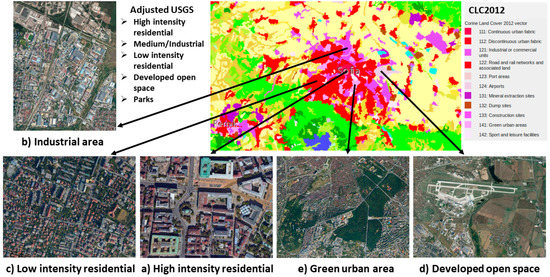
Figure 2.
Map of Corine land cover and images represented different urban categories in the adjusted USGS classes.
It is difficult to classify different urban areas due to the huge landscape diversity in Sofia city, but according classification of Stewart and Oke [54], the following build types are most appropriate.
(a) High intensity residential areas (the central part of the city) where people reside or work in high numbers. Impervious surfaces account for 80% to 100% of the total cover, a dense mix of 3–5 stories buildings with paved land cover and a few trees–category of compact midrise.
(b) Medium or industrial areas (mainly the northern and eastern part of the city) with the impervious surfaces account for 50% to 79% of the total cover. It is not a typical heavy industrial area, but mainly open arrangement of large low-rise buildings (1–3 stories) with low plants and bushes-large low-rise category;
(c) Low intensity residential areas (cover the largest part of the city) with the impervious surfaces accounting for 20% to 49% percent of the total cover, an open arrangement of low-rise buildings (1–3 stories), and midrise buildings (3–18 stories) in large residential complexes, with low plants and scattered trees - open midrise or low-rise category;
(d) Developed open space (the airport, roads, construction sites, sport and leisure facilities ets.) areas with a mixture of some constructed materials, but mostly vegetation in the form of grasses and low bushes. Impervious surfaces account for less than 20% of total cover.
(e) Parks—we consider city green areas from the Corine land cover as mixed forest, which is most appropriate for parks in Sofia (see Figure 2e).
The interaction at the bottom model boundary between the surface and the atmosphere, that is, the coupling through surface fluxes of heat, moisture, and momentum, was performed by the Land Surface Model (LSM), a module in WRF. In addition to the computation of surface fluxes, LSMs also compute soil and land cover properties, such as soil temperature and moisture. WRF model provides output for main fluxes at the ground–surface sensible, latent heat and ground heat fluxes that balanced the total net radiation (incoming and outgoing shortwave and longwave radiation). Different land categories have diverse surface thermal properties such as thermal inertia, surface heat capacity, surface emissivity, and albedo (see Table 1). These values, related to the properties of land use categories, were derived from a composite of images assembled from satellite observations (Landsat) within the US National Land Cover Database (NLCD 2006). We understand that satellite-derived data are surface radiant temperatures of only those surfaces seen by the radiometer [55], mostly roofs in urban areas and modelling results should be commented with some degree of uncertainties.
We have applied the default BULK (1D) parametrization in this study. Using a sophisticated urban model, like a single layer urban canopy model (SLUCM; uses a two-dimensional street canyon to explicitly parameterize canyon radiative transfer, turbulence, momentum, and heat fluxes) or building effect parameterization (BEP; treats urban surfaces three-dimensionally, and considers heat in the buildings and the effects of vertical and horizontal surfaces on temperature, momentum, and turbulent energy) would improve thermal and mechanical properties of urban categories based on building morphology; we plan to use such complex urban schemes in the future. However, there has not been much urban research performed on urban morphological properties of Sofia. We acknowledge the above arguments as shortcomings and advise readers to keep this limitation in mind when reading this study with. At the same time, the sensitivity experiments of replacing the natural areas with urban land use, and further, with high density residential areas in Sofia, are informative and valuable contributions to urban planning.
This study is an ideal example for evaluating urban hotspots in the Sofia city and modeling future urban expansion. Here, we performed two different experiments to evaluate the different urban sensitivity to changing land use: (1) substitution of the urban area with most representative rural land cover; (2) replacement of existing built-up area (all four urban categories) with high-density residential land cover throughout the whole city. These sensitivities can inform urban planning activities in Sofia and provide a quantitative assessment to different configurations of urban development in Sofia.
2.2. Model Set-up
The study used the Advanced Research version of the Weather Research and Forecasting (ARW-WRFv3.9) model for the numerical experiments. ARW-WRF is a state-of-the-art atmospheric modeling system, designed for a broad range of applications [56]. We used four nested domains based on a lambert projection (Figure 3). Outermost domain 1 (D1) covers the Balkan Peninsula, intermediate domain 2 (D2) covers Bulgaria, domain 3 (D3) covers Western part of Bulgaria, and the innermost domain (D4) covers the Sofia Valley. D1 has 36 × 44 horizontal grid points with 32-km grid-point spacing; D2—73 × 65 with 8-km cells; D3—69 × 97 with 2-km cells, and D4 with 157 × 129 cells with 500 m. The model was implemented with 50 or 99 pressure-based terrain-following vertical levels from the surface to 50 Pa.
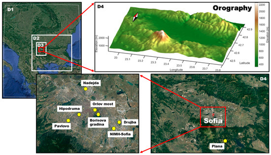
Figure 3.
Modeling domains with an enlarged view of the innermost domain D4 and Sofia city; the location of observational sites used for model validation are also shown.
The initial and boundary conditions were derived from the 0.25-degree NCEP Final Operational Model Global Tropospheric Analyses datasets [57] available every 6 hours. This product comes from the Global Data Assimilation System, which continuously collects observational data from the Global Telecommunications System. Data assimilation (fdda model option) was used for the outermost domain D1 for all vertical levels. Intermediate domains D2 and D3 used data assimilation for the first 10 model levels from the ground. We did not apply data assimilation for the innermost domain (Sofia Valley).
The selected case study covered 11 days (25 August–4 September 2016) with an additional 24 hours of spin-up. The period is characterized with anticyclonic fair weather, dry (low humidity, the mixing ratio 7 g/kg or approximately 48% relative humidity, averaged for all stations in Sofia) and quiescent (wind speed < 5 m/s at 850-hPa) conditions.
The WRF physics package included the Rapid Radiative Transfer Model (RRTM) longwave radiation parameterization [58] and Dudhia shortwave radiation parameterization [59] to compute radiation at every 10 minutes and Noah land surface model [60]. Grell-Freitas (GF) cumulus scheme [61] was used only for domains D1 and D2. The same domain has been tested already with different planetary boundary layer (PBL) and moisture schemes [50,62]. A sophisticated scheme Lin et al. [63], suitable for real-data high-resolution simulations, and three of the available in the model PBL schemes (with their corresponding surface schemes) were considered after preliminary comparison against observations in previous studies. Three selected PBL schemes were tested in this study: the Yonsei University scheme, YSU [64], the Mellor–Yamada–Janjic scheme, MYJ [65], the Bougeault and Lacarrere scheme, BouLac [66]. These PBL schemes provide the most reasonable agreement with observations from the preliminary tests, where all available options have been tested.
2.3. Observations
Observations were available for temperature and relative humidity at 2 m, wind speed, and direction at 10 m, and surface and soil temperature at 10 cm depth for three different sites. The radiosonde of the atmosphere is held in National Institute of Meteorology and Hydrology, Bulgarian Academy of Sciences (NIMH-BAS) by using the “DigiCoraIII” (Vaisala) system, and the measurements provided representative information on every second about temperature, humidity and wind in PBL with vertical resolution approximately 5 meters. However, these measurements were taken only once a day (at 12 UTC).
All available observations were used to estimate the model performance. Six automatic stations (Borisova Gradina, Orlov most, Druzhba, Hipodruma, Nadezhda, Pavlovo), and one synoptic station NIMH-Sofia (measurements on every 3 hours) in Sofia were used to calculate the near surface statistics. One of the sites (NIMH-Sofia) provided radiosonde data for vertical profiles in comparison to the main meteorological variables, while three of the sites measured data for the soil temperature at 10 cm depth (Borisova Gradina, Plana, NIMH-Sofia).
The images that describe the observational site locations illustrating the typical city land use classes for Sofia are shown in Figure A1. More of the observation sites are located in the residential areas (Drujba, Hipodruma, Nadejda, Pavlovo) with specific morphology of the building structures. The NIMH site is a synoptic site located in an open area in agreement with the requirements of the World Meteorological Organization. The surrounding field measurement area is covered with small or medium-sized buildings, grass, bushes and short, woody trees and correspond to the class of sparsely built. The last site is located inside the biggest park in Sofia–Borisova gradina, which is covered by a heavily wooded landscape of deciduous trees. All parks in the study have been designated as mixed forest as this is very typical for Sofia city.
3. Results
3.1. Model Validation
Model performance was estimated using all available data—from the surface (Table 2), the soil (Table 3) and the upper air observations (Table 4). The surface observations were taken at standard height 2 m for temperature and relative humidity. The land-surface model was also validated by the soil temperature (Table 3) at 10 cm depth. The vertical statistics were calculated using the nearest to the model level data from the radiosonde profile, as the observations are taken with fine (~5 m) resolution (Table 4). Standard statistical measures—the mean bias (MB) and error (ME), root mean square error (RMSE), and correlation coefficient (r) are shown together with the mean values and standard deviation. The indexes of agreement (IA) parameter developed by Willmott [67] is a standardized method to determine the degree of the model prediction error (see Equation (1))
where and are the predicted and observed values, respectively, and is the mean observed value. The IA values range between zero and 1, with 1 indicating a perfect match.
Table 2.
Statistical measures for near-surface variables for three PBL schemes at all six stations.
Table 3.
Statistical measures for the soil temperature at 10 cm depth for three PBL schemes.
Table 4.
Statistics for the upper model levels (up to 2000 m) at NIMH-Sofia location (12 UTC).
Three different PBL schemes (i.e., BouLac, MUJ and YSU) were statistically compared. All PBL schemes provided relatively similar results with excellent performance for the temperature at 2 m height (Table 2) and for upper levels (Table 4). There were slight negative biases of less than 1 °C. The IA and r values were above 0.95 for all PBL schemes. The soil temperature at 10 cm depth (Table 3) was also captured well in the city area at Borisova Gradina, with r above 0.9, but not so well at the Plana site (r > 0.75). Plana is situated on a mountain plateau at a higher elevation in comparison with Sofia (between 530 and 610 ASL). The simulated soil temperature showed consistent negative biases of less than 1.5 °C at the high elevation, and positive biases around 1–2 °C in the Sofia city.
Unlike temperature, the mixing ratio was not in a good agreement with observations, showing a systematic under-prediction of humidity. The rates of IA were between 0.73–0.75 and the correlation coefficient was approximately 0.6 (Table 2).
Note that wind speed and wind direction were not evaluated within the city, as the observed stations were unable to capture the mean city flow characteristics due to obstruction from buildings. Due to this reason the wind speed was validated only from the upper level air measurements in Table 4. These statistics in Table 4 are not unexpected, because this study considered weak wind conditions that led to significant variations, especially in the wind speed, as the probe was flying with the turbulent eddies, and the actual profile was not an average characteristic (10 min).
Examples of time series for surface meteorological parameters at selected locations and vertical profiles are shown in Appendix A. The model captured the vertical profiles of temperature (Figure A2) and wind direction (Figure A5) well. However, model underestimated the mixing ratios (Figure A3) and wind speed (Figure A4) within PBL for August 27th and 28th 2015. Generally, differences between model results applying different PBL schemes are pronounced in the velocity field. BouLac and MYJ produced the lowest and highest wind speeds respectively for the selected cases (Figure A4b). Even with 50 vertical levels detailed boundary layer flow structure was not captured well by the model. For this reason, a new experiment with the relatively best performing YSU PBL scheme was performed with 99 vertical levels to capture the vertical profile of the wind field (Figure A4, Figure A5). Table 4 shows the significant improvement in model results due to the increase in the number of vertical levels.
The general trend in the diurnal temperature evolution (Figure A6) was captured well by the model except for the extreme minimum and maximum temperatures values. WRF captured the trend in the mixing ratio with a decrease in value on August 28th–29th 2015, and an increase at the end of the study period. Time series for the wind speed and direction are shown only for the official synoptic station NIMH-Sofia (note, here measurements were not affected significantly by the buildings). The best performance for wind speed was found for YSU scheme (Figure A8). The main differences occurred during the night when WRF simulated the quiescent conditions, but measurements were registered as the whole numbers, and thus showed zero wind speed. Model predictions for wind are more difficult to evaluate using measurements taken at a single point, given the sub-grid inhomogeneity of the velocity vector within a grid area, much more than with temperature and humidity [13,28]. The model cannot resolve this variability with the 500 m grid.
The performance of different PBL schemes in simulating the PBLH is critical, as it provides an integral estimation of the model abilities to describe turbulent processes in PBL. Figure 4 shows a comparison between simulated PBLH for three PBL schemes and calculated from observations using different methods. Each PBL scheme itself use different criteria to estimate the PBLH. BouLac is a 1.5th-order closure scheme, and the non-local transport of heat is considered in the convective boundary layer, allowing the slightly stable stratification persisting with upward heat flux. The BouLac scheme defines the PBLH at the height where the virtual potential temperature (θv) is 0.5 K higher than in the first eta level. MYJ is a 1.5th-order closure scheme considering local vertical mixing process. A prescribed turbulent kinetic energy (TKE) value of 0.1 m2/s2 is used to define the PBLH. The YSU is a non-local-K scheme with explicit entrainment layer and parabolic K profile in the unstable mixed layer. This scheme considers entrainment at the top of the PBL, and different thresholds of bulk Richardson number (Rib) are used to determine the top of stable and unstable PBLH.
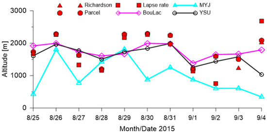
Figure 4.
PBLH comparison for different PBL schemes along with various methods of retrieving PBLH from observations.
To retrieve PBLH from the radiosonde measurements, different methods have been applied. The Richardson [68] and Parcel [69] methods overlap almost for all cases (except for September 3rd). For some days the Lapse rate method also provides similar results to the other described methods. The variance in PBLH estimation provided by different PBL schemes depends strongly on the criteria that they have used. Both schemes (BouLac and YSU) use virtual potential temperature and provide similar results; the MYJ allows only local transport and prescribes turbulent kinetic energy value ensure lower PBLH. All PBL schemes overestimated the wind speed on August 27th, 30th and September 2nd–4th 2015 at NIMH–Sofia (see Figure A7). It is likely to affect the surface temperature by cooling and reduce convective motion, leading to underestimation of PBLH calculated from MYJ for these days (Figure 4). Many studies [70,71] found that the non-local schemes provide warmer, drier and deeper daytime PBLs than the local MYJ scheme because non-local transport enhances the vertical mixing and entrainment. Our study confirmed the previous findings with MYJ underestimating the PBLH in comparison to other schemes.
4. Numerical Experiments
The simulation set-up is described in Section 2.2. We selected the YSU scheme for the following experiments because it is a simple, unique, and widely used scheme that allows nonlocal vertical transport. All new experiments are performed using more vertical levels (99), thereby ensuring better model performance (see Table 4 and Figure A2, Figure A3, Figure A4 and Figure A5).
Four different built-up categories (high and low-intensity residential areas, medium or industrial areas, and developed open space—roads, parking, airport, sport and leisure facilities, etc.) were considered for the urban area in this study for so called further base urban case (Figure 5a). This case is validated in Section 3.1 as it corresponds to the real present conditions. Two more numerical experiments were conducted, with the corresponding abbreviation used further: (1) non-urban case—all urban categories in Sofia area are replaced with the surrounding the city most common land cover category-Dryland Cropland and Pasture (Figure 5b); and (2) urban-high-intensity case—all four built-up categories were replaced with high-intensity residential areas (Figure 5c). The difference in model fields between base urban and non-urban cases provided better understanding of the effect of urbanization on local meteorological conditions. The changes in model fields between urban-high-intensity and base urban cases describe the hypothetic city expansion. We realize that the defined scenarios are exaggerated to some extent, but the goal of this study is to draw attention to possible adverse effects on our environment due to land use change on one hand, and, on the other, the expansive building construction in Sofia city during the past couple of decades, producing many very densely built-up spots.
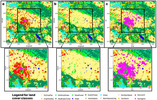
Figure 5.
Maps of land cover classes used in different numerical experiments: a base urban case with four built-up CORINE categories (a); non-urban case (b), urban-high-intensity case (c).
A box-and-whisker diagram is a descriptive method for graphically depicting groups of numerical data through their quartiles. Figure 6 presents the differences between base urban and non-urban scenarios. Plots describe the mean (red dot inside the box), the median (black line inside the box), the vertical lines correspond to the lowest datum still within 1.5IQR (interquartile range) of the lower quartile (base of the box) and the highest datum still within 1.5IQR of the upper quartile (top of the box). Dots present all data outside the adopted criterion. Data, extracted from all grids with built-up land cover, considering the entire period were used to calculate the statistics.
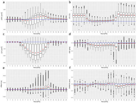
Figure 6.
Box plots presenting differences between base urban and non-urban scenarios for sensible heat flux (a), temperature (b), latent heat flux (c), water vapor mixing ratio (d), PBL height (e) and wind speed at 10 m (f). Data are extracted from all grids with built-up land use and cover the entire considering period.
The effect of urbanization (the expansion of the urban landscape) leads to significant disturbance of the surface geometry and properties. Natural materials are removed, replaced or modified, and the new environment is often dominated by impermeable manufactured materials. The difference in sensible heat flux due to surface cover modifications had a maximum mean value more than 100 W/m2 around noon when the maximum solar radiation is expected (Figure 6a). The urbanization led to an increase of approximately 2.5 °C in 2 m temperature during the night, when the urban structures emit the daytime stored heat, well-known as heat island effect (Figure 6b). The urban landscapes are the predominant impervious surface cover, and the relative lack of vegetation means there is relatively little water available for evapotranspiration, so the daytime latent heat flux is significantly reduced. The decrease in the latent heat flux means value close to 200 W/m2 (Figure 6c) affect the moisture content in the atmosphere, and the water vapor mixing ratio drops with approximately 1g/kg (Figure 6d) during the daytime. Data for the PBLH were more scattered out of the datum 1.5IQR (quartile range) because PBLH depends on many different factors and they have random variations during the study period. An effect on the increase of the PBL depth due to the presence of buildings was observed in the late afternoon when the convection is fully developed (Figure 6e). The study period covered days with calm conditions and weak wind, but a slight decrease in speed was registered in the late afternoon and early evening hours (Figure 6f).
The second experiment considered all four built-up categories to be replaced with high-intensity residential areas. A significant difference in sensible heat flux with maximum mean value more than 100 W/m2 was simulated in the morning hours (Figure 7a). The growth of building density and height led to a slight increase in the near-surface temperature ~1 °C in the morning, and a decrease during the afternoon (after 16 UTC) and night ~2.5 °C (Figure 7b). A small growth in the latent heat flux value with approximately 20 W/m2 (Figure 7c) was simulated in the morning hours. There were no significant changes for water vapor mixing ratio (Figure 7d), a small increase in morning PBLH (Figure 7e) and wind speed reduction in the afternoon due to an increase of the surface roughness (Figure 7f).
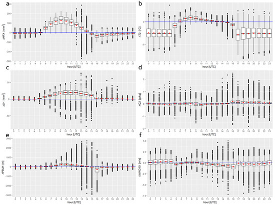
Figure 7.
Box plots presenting differences between urban-high-intensity and base urban scenarios for sensible heat flux (a), temperature (b), latent heat flux (c), water vapor mixing ratio (d), PBL height (e) and wind speed at 10 m (f). Data are extracted from all grids with built-up land use and cover the entire considering period).
These results are quite unexpected, considering the behavior related to the temperature and moisture. A number of previous studies concluded that the high density of building structures increases the UHI intensity and decrease the soil moisture [54,55,72,73]. UHI is strongly correlated with the density of urban use, the warmest areas are linked with the greatest conversion to urban development, especially those densely built-up with deep street canyons [54,73]. Hence, the high-rise, high-density city experiences a temperature cycle with a small daily temperature range [74].
Diurnal evolution of different variables for all three cases (non-urban, urban base and urban-high-intensity) are shown if Figure 8. The nocturnal temperature is substantially reduced for urban-high-intensity in comparison with the urban base case, leading to weakness of the UHI effect (Figure 8b). Our hypothesis is that higher surface absorptivity during the day (the surface albedo is reduced) increases the temperature in the morning hours. The higher obstacles produce a greater amount of mechanically induced turbulence in the late afternoon hours and cool the surface (at 16–17 UTC), which reduced the skin and near surface temperature. The cooling in the afternoon stores less heat in urban surfaces (different urban categories have the same surface heat capacity according to Table 1) reducing the surface emissivity during the night for the high-intensity urban category, that decrease the diurnal amplitude. The water vapor mixing ratio is similar for both urban and high-intensity urban cases. The moisture during the day is much lower for urban cases in comparison with the non-urban case (Figure 8d). The increase in sensible and latent heat fluxes, PBL height and decrease in wind speed are in agreement with previous studies.
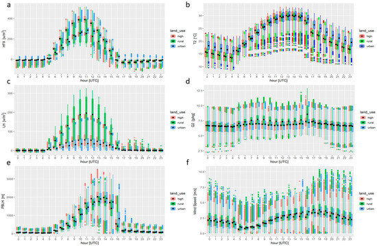
Figure 8.
Box plots presenting the diurnal evolution of sensible heat flux (a), temperature (b), latent heat flux (c), and water vapor mixing ratio (d), PBL height (e) and wind speed at 10 m (f). Data are extracted from all grids with built-up land use and cover the entire considering period).
The main reason for the unexpected temperature diurnal evolution is most likely that the thermal properties for different urban classes are not described properly using the BULK (1D) urban parameterization, and the modelled thermal response is unrealistic. The surface heat capacity denotes the ability of a material to store heat, and this parameter is the same for all urban categories in the used bulk parametrization. In paper of Göndöcs et al. [40] the authors found quite a big difference for the heat capacity of walls and roofs that is not taken into account with the BULK (1D) urban parameterization.
Figure 9 and Figure 10 show spatial distribution that corresponds to time with a maximum of the mean value according to plots in Figure 6 and Figure 7. All experiments include the entire period of study (11 days), and the mean fields represent an hourly average over all days. Examples of the spatial distribution of differences in average fields of sensible heat and latent fluxes, temperature and water vapor mixing ratio, PBLH and u* in similarity theory (parameter related to mechanically induced turbulent stress) are shown.
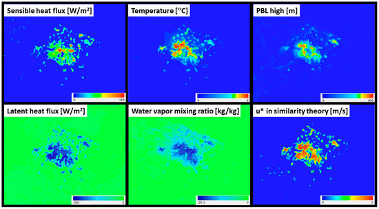
Figure 9.
Spatial distribution of maximum observed differences between variables from the model output related to base urban and non-urban cases for specific selected characteristics.
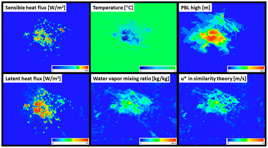
Figure 10.
Spatial distribution of maximum observed differences between variables from the urban-high-intensity and base urban cases for specific selected characteristics.
The results from experiment 1 (the difference between variables from the model output related to base urban and non-urban cases) are shown in Figure 9, and from experiment 2 (the difference between variables from the urban-high-intensity and base urban cases) in Figure 10.
Maximum effect from the experiment 1 in the fields of sensible heat flux appeared at 1 pm UTC (3 pm local time), which correspond to strong solar radiation and significant difference in land surface parameters–decrease in albedo, surface emissivity, thermal inertia, and surface heat capacity for the urban area (see Table 1). The most substantial was the difference in high-intensity residential areas and developed open spaces (see Figure 5). The latent heat flux was reduced approximately 200 W/m2 (Figure 9) due to the decrease in soil moisture availability 2–3 times (see SLMO in Table 1) between different urban categories. The maximum difference was registered at 11 am UTC (1 pm local time). The urban landscape increased the temperature with 5 °C in the central part of the city (at 5 pm UTC; 7 pm local time), and decreased moisture with 2 g/kg in comparison with the rural area (at 4 pm; 6 pm local time). Built-up areas have very high surface roughness lengths, especially for high intensity residential and medium or industrial areas (see SFZ0 in Table 1) and an increase in PBLH with approximately 900 m and higher friction velocity (over the all urban categories, except developed open space) is seen (Figure 9). The maximum differences were simulated at 4 pm UTC (6 pm local time) when the convective boundary layer was fully developed.
High-intensity residential areas, i.e., tall buildings and denser arrangements of buildings, strengthen the effect of urbanization. An additional increase in sensible heat flux due mainly to the developed open space category as the differences in land cover parameters were more significant in comparison with the high-intensity residential area (see Table 1). It is different for the latent heat flux, where contribution have only medium or industrial and low-intensity residential areas (the developed open space category has the same soil moisture availability as the high-intensity residential area). The increase in sensible heat flux was more significant ~180 W/m2 than latent heat flux ~30 W/m2 (Figure 10). Changes in water vapor mixing ratio were minimal, but changes in temperature were significant in the late afternoon and during the night. Faster cooling of the high-intensity residential areas in comparison with other categories led to a lower near surface temperature that produce the negative difference of ~2 °C for some areas at 5 pm UTC (7 pm local time). Tall buildings and the dense, built-up urban environment added to the increase in PBLH, with approximately 400 m for the central city area and an increase in friction velocity (Figure 10).
5. Conclusions
Most of the earth’s resources are consumed in the megacities of today, in which most people live. Numerical modeling techniques are compelling tools that deliver critical data to city planners and stakeholders for decision making [75,76]. The implementation in our calculations of CORINE 2012 Land Cover data, the most recent dataset, ensured a better description of current urban areas. High resolution of the land cover data provided the flexibility to increase model horizontal grid resolution to 500 m and update the land cover, and thus, to accurately represent surface characteristics. Different land categories have diverse surface thermal properties which are very important for such types of studies. Model verification showed that resolved configuration provides reliable and trustworthy model results, and also that increasing the number of vertical levels improve the model results.
Both described experiments provided useful information on the influence of urbanization by modifying agricultural land to the urban, built-up areas. The first experiment (all urban categories in Sofia were replaced with the most common land cover category surrounding the city) showed that urbanization can increase air temperatures by 5 °C and decrease moisture by 2 g/kg in the central area of Sofia. The sensible heat flux rose by more than 100 W/m2 and the latent heat flux was reduced by approximately 200 W/m2. Replacing rural with urban land also affected the PBLH (~900 m higher than over the rural area) and reduced the wind speed in the afternoon. Human activities make our cities drier, decrease temperature diurnal amplitude, increase turbulent stress and PBLH, and make our living environment unfavorable.
The second experiment (all four built-up categories were replaced with high-intensity residential areas), corresponded to a hypothetical city development expansion. It was found that changes in urban structure, building height, and denser, built-up areas further contribute to the sensible heat flux by more than 100 W/m2 in the morning hours and to PBLH (~400 m). The latent heat flux also rose by 30 W/m2 during daytime, showing an additional stress over the urban environment. The results relating to temperature diurnal evolution were unexpected, and were most likely due to the improperly described thermal properties for different urban classes that were used with the BULK (1D) urban parameterization. We are in the process of developing improved urban morphological properties and characteristics that are missing for small cities, such as Sofia, which have experienced sudden population and infrastructure growth. We are confident that this study provides motivation for such datasets to develop detailed urban heat mitigation and assessment studies for small cities with new urban environmental problems.
Urban environmental challenges need to be solved promptly and in parallel with the city planning to ensure a sustainable future. To the best of our knowledge, both numerical experiments, together with the implementation of the most recent dataset, have been done for the first time for Sofia in this paper. This work is an example of an integrated urban system approach that can help to create well-planned cities, to support future increasing populations and environmental problems related to human activity, and to consider health and comfort of the city inhabitants. Green and blue infrastructure (GBI) has the potential to tackle the issue of environmental protection by maintaining healthy ecosystems, reconnecting fragmented natural areas and restoring damaged habitats, as well as the social challenges. Permeable paving using modular blocks, car parking spaces with grass cover, white painted or green rooftops and green building facades are only a few examples for which the potential of different designed numerical experiments exists in support of city managers. This approach can allow cities to avoid costly and harmful mistakes due to a lack of proper expansion planning. Human health and comfort are very interesting topics that may be the subject of future research.
Author Contributions
To the conceptualization and methodology have contributed R.D. and V.D.; for software—E.V.; for validation—R.D.; for formal analysis—V.D. and E.E.; for investigation, R.D. and E.V.; for data curation V.D., O.G. and D.I.; writing—original draft preparation, R.D.; writing—review and editing, A.S.
Funding
This research and APC was funded by Research Fund at the Bulgarian Ministry of Education and Science, grant number DN4/7 (Study of the PBL structure and dynamics over complex terrain and urban area). Ashish Sharma was supported by NSF-CBET award 1929856, and DOD award W911NF-19-1-0199.
Acknowledgments
We acknowledge the provided access to the e-infrastructure of the NCDSC–part of the Bulgarian National Roadmap on RIs, with the financial support by the Grant No D01-221/03.12.2018. This paper reflects the views of the authors and not necessarily those of the funding agency and author’s affiliated institutions.
Data Availability
Data used to support the findings of this study are available from the corresponding author upon request.
Conflicts of Interest
The authors declare no conflict of interest.
Appendix A

Figure A1.
Maps of the observational sites location with surrounding morphology of the building structures and land cover.

Figure A2.
Temperature profiles for the entire modeling domain (a) and in PBL (b) for selected days at 12 UTC, NIMH-Sofia site.

Figure A3.
Mixing ratio profiles for the entire modeling domain (a) and in PBL (b) for selected days at 12 UTC, NIMH-Sofia site.

Figure A4.
Wind speed profiles for the entire modeling domain (a) and in PBL (b) for selected days at 12 UTC, NIMH-Sofia site.

Figure A5.
Wind direction profiles for the entire modeling domain (a) and in PBL (b) for selected days at 12 UTC, NIMH-Sofia site.

Figure A6.
Time series for temperature at selected locations in Sofia—3 suburban sites (Druzhba, Hipodruma, Nadejda) and a traffic urban site (Pavlovo).

Figure A7.
Time series for mixing ratio at selected locations in Sofia—3 suburban sites (Druzhba, Hipodruma, Nadejda) and a traffic urban site (Pavlovo).

Figure A8.
Time series for wind speed and direction at NIMH site in Sofia.
References
- United Nations. DESA/Population Division World Urbanization Prospects: The 2018 revision. Available online: https://www.un.org/development/desa/publications/2018-revision-of-world-urbanization-prospects.html (accessed on 20 May 2019).
- Bulgarian National Statistical Institute. Population and Demographic Processes 2017. Available online: http://www.nsi.bg/sites/default/files/files/publications/DMGR2017.pdf (accessed on 20 May 2019).
- Penev, L.; Niemelä, J.; Kotze, J.; Chipev, N. Ecology of the City of Sofia: Species and Communities in an Urban Environment, 1st ed.; Penev, L., Niemelä, J., Kotze, J., Chipev, N., Eds.; Pensoft: Sofia, Bulgaria, 2004; p. 456. [Google Scholar]
- Hirt, S. Suburbanizing Sofia: Characteristics of Post-Socialist Peri-Urban Change. J. Urban Geography 2007, 28, 755–780. [Google Scholar] [CrossRef]
- Geshkov, M. Urban Sprawl in Eastern Europe. The Sofia City Example. Economic Alternatives 2015, 2, 101–116. [Google Scholar]
- Bulgarian National Statistical Institute. Cities and their urbanised areas in the republic of Bulgaria. Report, Eurostat/EC Grant N°08141.2013.001-2013.646. Available online: http://www.nsi.bg/sites/default/files/files/ publications/URBAN_ENG.pdf (accessed on 20 May 2019).
- World Bank Group Urban, Social, Rural and Resilience Global Practice. Available online: http://documents.worldbank.org/curated/en/322891511932837431/pdf/121724-BRI-P154478-PUBLIC-Bulgaria-Snapshot-PRINT.pdf (accessed on 20 May 2019).
- Georgieva, M. Sustainable Development of Urban Spaces in Bulgaria: Theoretical Aspects. Trakia J. Sci. 2015, 13, 49–53. Available online: http://tru.uni-sz.bg/tsj/Vol.%2013,%202015,%20Suppl.%201,%20Series%20Social%20Sciences/SF/SF/reg.razv/M.Georgieva.pdf (accessed on 3 May 2019). [CrossRef]
- Vitanova, L.; Kusaka, H. Study on the Urban Heat Island in Sofia City: Numerical Simulations with Potential Natural Vegetation and Present Land Use Data. Sustain. Cities Soc. 2018, 40, 110–125. [Google Scholar] [CrossRef]
- Oke, T.R.; Mills, G.; Christen, A.; Voogt, J.A. Urban Climates, 1st ed.; Cambridge University Press: Cambridge, UK, 2017. [Google Scholar]
- Oke, T.R. Boundary Layer Climates, 2nd ed.; Methuen: New York, NY, USA, 1988. [Google Scholar]
- Fernando, H.J.S.; Zajic, D.; Di Sabatino, S.; Dimitrova, R.; Hedquist, B.; Dallman, A. Flow, turbulence, and pollutant dispersion in urban atmospheres. Phys. Fluids 2010, 22, 051301. [Google Scholar] [CrossRef]
- Sharma, A.; Fernando, H.J.S.; Hamlet, A.F.; Hellmann, J.J.; Barlage, M.; Chen, F. Urban meteorological modeling using WRF: A sensitivity study. Int. J. Climatol. 2017, 37, 1885–1900. [Google Scholar] [CrossRef]
- Sharma, A.; Woodruff, S.; Budhathoki, M.; Hamlet, A.F.; Fernando, H.J.S.; Chen, F. Can green roofs reduce urban heat stress in vulnerable urban communities: A coupled atmospheric and social modeling approach? In Proceedings of the AGU Fall Meeting, New Orleans, LA, USA, 11–15 December 2017; Available online: http://adsabs.harvard.edu/abs/2017AGUFMGC11E..01S (accessed on 30 June 2019).
- Hunt, J.C.; Timoshkina, Y.V.; Bohnenstengel, S.I.; Belcher, S. Implications of climate change for expanding cities worldwide. Available online: http://centaur.reading.ac.uk/28480/1/Hunt_etal_2012.pdf (accessed on 30 June 2019).
- Emmanuel, R.; Fernando, H.J.S. Effects of urban form and thermal properties in urban heat island mitigation in hot humid and hot arid climates: The cases of Colombo, Sri Lanka and Phoenix, USA. Clim Res. 2007, 34, 241–251. [Google Scholar] [CrossRef]
- Basara, J.B.; Basara, H.G.; Illston, B.G.; Crawford, K.C. The impact of the urban heat island during an intense heat wave in Oklahoma City. Adv. Meteorol. 2010. [Google Scholar] [CrossRef]
- Li, D.; Bou-Zeid, E. Synergistic interactions between urban heat islands and heat waves: The impact in cities is larger than the sum of its parts. J. Appl. Meteorol. Climatol. 2013, 52, 2051–2064. [Google Scholar] [CrossRef]
- Sharma, A.; Conry, P.; Fernando, H.J.S.; Hamlet, A.F.; Hellmann, J.J.; Chen, F. Green and cool roofs to mitigate urban heat island effects in the Chicago metropolitan area: Evaluation with a regional climate model. Environ. Res. Lett. 2016, 11. Available online: https://iopscience.iop.org/article/10.1088/1748-9326/11/6/064004/meta (accessed on 30 June 2019).
- Keeler, J.M.; Kristovich, D.A.R. Observations of Urban Heat Island Influence on Lake-Breeze Frontal Movement. J. Appl. Meteorol. Climatol. 2012, 51, 702–710. [Google Scholar] [CrossRef]
- Sharma, A.; Fernando, H.J.S.; Hellmann, J.J.; Chen, F. Sensitivity of WRF Model to Urban Parameterizations, With Applications to Chicago Metropolitan Urban Heat Island. In Proceedings of the ASME 2014 4th Joint US-European Fluids Engineering Division Summer Meeting collocated with the ASME 2014 12th International Conference on Nanochannels, Microchannels, and Minichannels, Chicago, IL, USA, 3–7 August 2014. [Google Scholar] [CrossRef]
- Niyogi, D.; Pyle, P.; Lei, M.; Arya, S.P.; Kishtawal, C.M.; Shepherd, M.; Chen, F.; Wolfe, B. Urban Modification of Thunderstorms: An Observational Storm Climatology and Model Case Study for the Indianapolis Urban Region. J. Appl. Meteorol. Climatol. 2011, 50, 1129–1144. [Google Scholar] [CrossRef]
- Bouyer, J.; Inard, C.; Musy, M. Microclimatic coupling as a solution to improve building energy simulation in an urban context. Energy Build. 2011, 43, 1549–1559. [Google Scholar] [CrossRef]
- Conry, P.; Sharma, A.; Potosnak, M.; Leo, L.S.; Bensman, E.; Hellmann, J.; Fernando, H.J.S. Chicago’s heat island and climate change: bridging the scales via dynamical downscaling. In Proceedings of the ASME 2014 4th Joint US-European Fluids Engineering Division Summer Meeting collocated with the ASME 2014 12th International Conference on Nanochannels, Microchannels, and Minichannels, Chicago, IL, USA, 3–7 August 2014. [Google Scholar] [CrossRef]
- Conry, P.; Sharma, A.; Potosnak, M.J. Chicago’s heat island and climate change: Bridging the scales via dynamical downscaling. J. Appl. Meteorol. Climatol. 2015, 54, 1430–1448. [Google Scholar] [CrossRef]
- Zajic, D.; Fernando, H.J.S.; Brown, M.J.; Pardyjak, E.R. On flows in simulated urban canopies. Environ. Fluid Mech. 2015, 15, 275–303. [Google Scholar] [CrossRef]
- Dimitrova, R.; Sini, J.-F.; Richards, K.; Schatzmann, M.; Weeks, M.; Perez García, E.; Borrego, C. Influence of thermal effects on the wind field within the urban environment. Bound-Lay Meteorol. 2009, 131, 223–243. [Google Scholar] [CrossRef]
- Fernando, H.J.S.; Dimitrova, R.; Sentic, S. Climate Change Meets Urban Environment. In National Security and Human Health Implications of Climate Change NATO Science for Peace and Security Series C: Environmental Security; Fernando, H.J.S., Klaić., Z., McCulley, J.L., Eds.; Springer Science & Business Media: Berlin, Germany, 2012; pp. 115–133. [Google Scholar] [CrossRef]
- Changnon, S.A., Jr. Inadvertent weather modification in urban areas, lessons for global climate change. Bull. Am. Meteorol. Soc. 1992, 73, 619–627. [Google Scholar] [CrossRef]
- Kew, S.F.; Philip, S.Y.; van Oldenborgh, G.J.; Otto, F.E.L.; Vautard, R.; van der Schrier, G. The Exeptional Summer Heat Wave in Southern Europe 2017. B. Am. Meteorol. Soc. 2018, 100, S49–S53. [Google Scholar] [CrossRef]
- Mircheva, B.R. Terrestrial water storage anomaly during the 2007 heat wave in Bulgaria. Master’s Thesis, Sofia University “St. Kliment Ohridski”, Sofia, Bulgaria, April 2016. [Google Scholar]
- Livezey, R.E.; Tinker, R. Some meteorological, climatological, and microclimatological considerations of the severe US heat wave of mid-July 1995. B. Am. Meteorol. Soc. 1996, 77, 2043–2054. [Google Scholar] [CrossRef]
- Bouchama, A. The 2003 European heat wave. Intens. Care Med. 2004, 30, 1–3. [Google Scholar] [CrossRef]
- Patz, J.A.; Campbell-Lendrum, D.; Holloway, T.; Foley, J.A. Impact of regional climate change on human health. Nature 2005, 438, 310–317. [Google Scholar] [CrossRef]
- Harlan, S.L.; Brazel, A.J.; Prashad, L.; Stefanov, W.L.; Larsen, L. Neighborhood microclimates and vulnerability to heat stress. Soc. Sci. Med. 2006, 63, 2847–2863. [Google Scholar] [CrossRef] [PubMed]
- Fernando, H.J.S. Polimetrics: The quantitative study of urban systems (and its applications to atmospheric and hydro environments). Environ. Fluid Mech. 2008, 8, 397–409. [Google Scholar] [CrossRef]
- Shepherd, J.M.; Pierce, H.; Negri, A.J. Rainfall Modification by Major Urban Areas: Observations from Spaceborne Rain Radar on the TRMM Satellite. J. Appl. Meteorol. 2002, 41, 689–701. [Google Scholar] [CrossRef]
- Shepherd, J.M. A Review of Current Investigations of Urban-Induced Rainfall and Recommendations for the Future. Earth Interact. 2005, 9, 1–27. [Google Scholar] [CrossRef]
- Li, X.; Zhou, Y.; Asrar, G.R.; Imhoff, M.; Li, X. The surface urban heat island response to urban expansion: A panel analysis for the conterminous United States. Sci. Total Environ. 2017, 605, 426–435. [Google Scholar] [CrossRef] [PubMed]
- Göndöcs, J.; Breuer, H.; Pongrácz, R.; Bartholy, J. Urban heat island mesoscale modelling study for the Budapest agglomeration area using the WRF model. Urban Climate 2017, 21, 66–86. [Google Scholar]
- Giannaros, T.M.; Melas, D.; Daglis, I.A.; Keramitsoglou, I.; Kourtidis, K. Numerical study of the urban heat island over Athens (Greece) with the WRF model. Atmos. Environ. 2013, 7, 103–111. [Google Scholar] [CrossRef]
- Lin, C.Y.; Chen, F.; Huang, J.C.; Chen, W.C.; Liou, Y.A.; Chen, W.N.; Liu, S.C. Urban heat island effect and its impact on boundary layer development and land–sea circulation over northern Taiwan. Atmos. Environ. 2008, 42, 5635–5649. [Google Scholar] [CrossRef]
- Chen, F.; Yang, X.; Zhu, W. WRF simulations of urban heat island under hot-weather synoptic conditions: The case study of Hangzhou City, China. Atmos. Res. 2014, 138, 364–377. [Google Scholar] [CrossRef]
- Höppe, P. The physiological equivalent temperature—A universal index for the biometeorological assessment of the thermal environment. Int. J. Biometeorol. 1999, 43, 71–75. [Google Scholar]
- Belding, H.S.; Hatch, T.F. Index for evaluating heat stress in terms of resulting physiological strains. Heating Piping Air Cond. 1955, 27, 129–136. [Google Scholar]
- Yaglou, C.P.; Minaed, D. Control of heat casualties at military training centers. Arch. Indust. Health 1957, 16, 302–316. [Google Scholar]
- Fiala, D.; Havenith, G.; Bröde, P.; Kampmann, B.; Jendritzky, G. UTCI-Fiala multi-node model of human heat transfer and temperature regulation. Int. J. Biometeorol. 2012, 56, 429–441. [Google Scholar] [CrossRef] [PubMed]
- Taleghani, M.; Kleerekoper, L.; Tenpierik, M.; van den Dobbelsteen, A. Outdoor thermal comfort within five different urban forms in the Netherlands. Build. Environ. 2015, 83, 65–78. [Google Scholar] [CrossRef]
- Vladimirov, E.; Dimitrova, R.; Danchovski, V. Sensitivity of the WRF Model Results to Topography and Land Cover: Study for the Sofia Region; Annuaire de l’Université de Sofia “St. Kliment Ohridski”, Faculté de Physique: Sofia, Bulgaria, 2018; Volume 111, pp. 87–106. [Google Scholar]
- Giovannini, L.; Antonacci, G.; Zardi, D.; Laiti, L.; Panziera, L. Sensitivity of simulated wind speed to spatial resolution over complex terrain. Energy Procedia 2014, 59, 323–329. [Google Scholar] [CrossRef]
- Giovannini, L.; Zardi, D.; de Franceschi, M.; Chen, F. Numerical simulations of boundary-layer processes and urban-induced alterations in an Alpine valley. Int. J. Climatol. 2014, 34, 1111–1131. [Google Scholar] [CrossRef]
- CLC2012, EEA. Available online: https://land.copernicus.eu/pan-european/corine-land-cover/clc-2012 (accessed on 30 June 2019).
- Pineda, N.; Jorba, O.; Jorge, J.; Baldasano, J.M. Using NOAA AVHRR and SPOT VGT data to estimate surface parameters: Application to a mesoscale meteorological model. Int. J. Remote Sens. 2004, 25, 129–143. [Google Scholar] [CrossRef]
- Stewart, I.D.; Oke, T.R. Local climate zones for urban temperature studies. B. Am. Meteorol. Soc. 2012, 93, 1879–1900. [Google Scholar] [CrossRef]
- Roth, M.; Oke, T.R.; Emery, W.J. Satellite-derived urban heat islands from three coastal cities and the utilization of such data in urban climatology. Int. J. Remote Sens. 2007, 10, 1699–1720. [Google Scholar] [CrossRef]
- Skamarock, W.C.; Klemp, J.B.; Dudhia, J.; Gill, D.O.; Barker, D.M.; Duda, M.G.; Huang, X.Y.; Wang, W.; Powers, J.G. A Description of the Advanced Research WRF Version 3. NCAR Tech. Note NCAR/TN-475+STR 2008. Available online: https://opensky.ucar.edu/islandora/object/technotes%3A500/datastream/PDF/view (accessed on 30 June 2019). [CrossRef]
- NCEP Final Operational Model Global Tropospheric Analyses. Available online: http://rda.ucar.edu/datasets/ds083.2/ (accessed on 30 June 2019).
- Mlawer, E.J.; Taubman, S.J.; Brown, P.D.; Iacono, M.J.; Clough, S.A. Radiative transfer for inhomogeneous atmospheres: RRTM, a validated correlated-k model for the longwave. J. Geophys Res. Atmos. 1997, 102, 16663–16682. [Google Scholar] [CrossRef]
- Dudhia, J. Numerical study of convection observed during the winter monsoon experiment using a mesoscale two-dimensional model. J. Atmos. Sci. 1989, 46, 3077–3107. [Google Scholar] [CrossRef]
- Chen, F.; Dudhia, J. Coupling an advanced land surface-hydrology model with the Penn State-NCAR MM5 modelling system. Part I: Model implementation and sensitivity. Mon. Weather Rev. 2001, 129, 569–585. [Google Scholar] [CrossRef]
- Grell, E.; Grell, G.; Bao, J.-W. Experimenting with a convective parameterization scheme suitable for high-resolution mesoscale models in tropical cyclone simulations. Geophys. Res. Abstr. 2013, 15, EGU2013-5746-2. Available online: http://meetingorganizer.copernicus.org/ EGU2013/EGU2013-5746-2.pdf (accessed on 30 June 2019). [CrossRef]
- Egova, E.; Dimitrova, R.; Danchovski, V. Numerical study of meso-scale circulation specifics in the Sofia region under different large-scale conditions. Bul. J. Meteol. Hydrol. 2017, 22, 54–72. Available online: http://meteorology.meteo.bg/global-change/files/2017/BJMH_2017_vol_22_3-4/BJMH_v22_issue_3-4_eegova_numerical.pdf (accessed on 30 June 2019).
- Lin, Y.L.; Farley, R.D.; Orville, H.D. Bulk parametrization of the snow field in a cloud model. J. Appl. Meteorol. 1983, 22, 1065–1092. [Google Scholar] [CrossRef]
- Hong, S.Y.; Pan, H.L. Nonlocal boundary layer vertical diffusion in a Medium-Range Forecast Model. Mon. Weather Rev. 1996, 124, 2322–2339. [Google Scholar] [CrossRef]
- Janjic, Z. The step-mountain coordinate: Physics package. Mon. Weather Rev. 1990, 118, 1429–1443. [Google Scholar] [CrossRef]
- Bougeault, P.; Lacarrere, P. Parametrization of orography-Induced turbulence in a mesobeta–scale model. Mon. Weather Rev. 1989, 117, 1872–1890. [Google Scholar] [CrossRef]
- Willmott, C.J. On the validation of models. Phys. Geogr. 1981, 2, 184–194. [Google Scholar] [CrossRef]
- Vogelezang, D.; Holtslag, A. Evaluation and model impacts of alternative boundary-layer height formulations. Bound.-Layer Meteorol. 1996, 81, 245–269. [Google Scholar] [CrossRef]
- Holzworth, G.C. Estimates of mean maximum mixing depths in the contiguous United States. Mon. Weather Rev. 1964, 92, 235–242. [Google Scholar] [CrossRef]
- Hu, X.-M.; Nielsen-Gammon, J.W.; Zhang, F. Evaluation of three planetary boundary layer schemes in the WRF model. J. Appl. Meteor. Climatol. 2010, 49, 1831–1844. [Google Scholar] [CrossRef]
- LeMone, M.A.; Tewari, M.; Chen, F.; Dudhia, J. Objectively determined fair-weather CBL depths in the ARW-WRF model and their comparison to CASES-97 observations. Mon. Weather Rev. 2013, 141, 30–54. [Google Scholar] [CrossRef]
- Gallo, K.P.; Easterling, D.R.; Peterson, T.C. The influence of land use/land cover on climatological values of the diurnal temperature range. J. Climate 1996, 9, 2941–2944. [Google Scholar] [CrossRef]
- Wang, K.; Li, Y.; Wang, Y.; Yang, X. On the asymmetry of the urban daily air temperature cycle. J. Geophys. Res. Atmos. 2017, 122, 5625–5635. [Google Scholar] [CrossRef]
- Yang, X.; Li, Y.; Luo, Z.; Chan, P.W. The urban cool island phenomenon in a high-rise high-density city and its mechanisms. Int. J. Climatol. 2017, 37, 890–904. [Google Scholar] [CrossRef]
- Sharma, A.; Woodruff, S.; Budhathoki, M.; Hamlet, A.F.; Chen, F.; Fernando, H.J.S. Role of green roofs in reducing heat stress in vulnerable urban communities—A multidisciplinary approach. Environ. Res. Lett. 2018, 13, 94011. [Google Scholar] [CrossRef]
- Kristovich, D.A.; Takle, E.; Young, G.S.; Sharma, A. 100 years of progress in mesoscale planetary boundary layer meteorological research. Meteorol. Monogr. 2019. [Google Scholar] [CrossRef]
© 2019 by the authors. Licensee MDPI, Basel, Switzerland. This article is an open access article distributed under the terms and conditions of the Creative Commons Attribution (CC BY) license (http://creativecommons.org/licenses/by/4.0/).