Article

Uncertainties in Arctic Sea Ice Thickness Associated with Different Atmospheric Reanalysis Datasets Using the CICE5 Model

1
Korea Polar Research Institute, Incheon 21990, Korea
2
Division of Earth Environmental System, Pusan National University, Busan 46241, Korea
3
Division of Environmental Atmospheric Science, Pukyong National University, Busan 48513, Korea
4
Faculty of Science, Niigata University, Niigata 8050, Japan
*
Author to whom correspondence should be addressed.
Atmosphere 2019, 10(7), 361; https://doi.org/10.3390/atmos10070361
Submission received: 28 April 2019 / Revised: 28 June 2019 / Accepted: 28 June 2019 / Published: 30 June 2019
(This article belongs to the Special Issue Atmospheric Processes Shaping Arctic Climate)

Abstract

:
Reanalysis data are known to have relatively large uncertainties in the polar region than at lower latitudes. In this study, we used a single sea-ice model (Los Alamos’ CICE5) and three sets of reanalysis data to quantify the sensitivities of simulated Arctic sea ice area and volume to perturbed atmospheric forcings. The simulated sea ice area and thickness thus volume were clearly sensitive to the selection of atmospheric reanalysis data. Among the forcing variables, changes in radiative and sensible/latent heat fluxes caused significant amounts of sensitivities. Differences in sea-ice concentration and thickness were primarily caused by differences in downward shortwave and longwave radiations. 2-m air temperature also has a significant influence on year-to-year variability of the sea ice volume. Differences in precipitation affected the sea ice volume by causing changes in the insulation effect of snow-cover on sea ice. The diversity of sea ice extent and thickness responses due to uncertainties in atmospheric variables highlights the need to carefully evaluate reanalysis data over the Arctic region.

1. Introduction

There has been a dramatic change in the Arctic sea ice in recent years [1,2,3,4,5]. The extents of Arctic sea ice between 2007 and 2016 are all ranked within the top 10 for minimum sea ice; September 2012 had the smallest summer sea ice extent on record (3.63 × 10⁶ km2) while Autumn (October and November) Arctic sea ice thickness in the 2000s decreased to about a half of that in the 1980s [5]. This has been accompanied by an increased fraction of weaker and thinner sea ice, which is more susceptible to further melting [4,6,7].
Sea ice modeling is an important approach to accounting for these rapid changes [8] and understanding the underlying processes. Atmospheric and oceanic variables are required for sea ice models, yet atmospheric observational data are very limited in the Arctic, especially in the open ocean where observations were scarce in time and place. As an alternative, atmospheric reanalysis data, which assimilate both in-situ and remote sensed observations, are often used to force sea ice models [9]. However, all reanalysis data for the Arctic region contain large uncertainties because of the remoteness of the region and the difficulty to observe [10,11,12,13]. As sea ice models are sensitive to surface forcings, uncertainties within the reanalysis data could lead to errors and biases in estimated sea ice variables such as concentration, thickness and volume and reduce the reliability of simulated results [10,14,15].
Efforts have been made to verify reanalysis data for the Arctic region and improve their quality using in-situ observations. For instance, Walsh et al. [16] showed that seasonality in cloud observation data from the Soviet Union’s North Pole drifting station was not captured by data from the National Center for Environmental Prediction Reanalysis 1 (NCEP R1). They also found that the correlation between cloud cover and temperature simulated by ERA-15 data was smaller than that between the corresponding observed data for that region. Makshtas et al. [17] confirmed that NCEP R1 did not adequately represent the state of the Arctic region because of large errors in its surface air temperature, specific humidity, and cloud cover measurements for summer, compared with the drifting station data. Screen and Simmonds [9] verified that Arctic temperature trends and profiles suggested by the ERA-40 data were less accurate than those indicated by satellite observations. Lüpkes et al. [18] also affirmed the existence of a large warm bias in the central Arctic in the ERA-Interim reanalysis data using ship-based observations.
Furthermore, previous studies have shown that all reanalysis data are subject to large amounts of uncertainties in radiative fluxes and precipitation [10,15]. According to Chaudhuri et al. [10], no reanalysis data pertaining to the Arctic region had a high correlation with observations, and large differences appeared in reanalysis data for long and shortwave radiation, wind, and precipitation. According to Lindsay et al. [15], characteristics of uncertainty for reanalysis data vary between variables, seasons, and surface conditions.
The Arctic sea ice is highly sensitive to the atmospheric forcing [14,15,19]. Its concentration is also susceptible to forcings, particularly in the summer, though it is not as susceptible as sea ice thickness. Variations and trends of the Arctic sea ice thickness are thermodynamically driven [20]. Wind forcing plays an important role in sea-ice re-distribution and dynamic thickening via deformation processes [21]. Snow is a good insulator and reflector that plays an important role in determining sea ice thickness [22] as thin (thick) snow cover over sea ice enhances (slows down) ice growth in winter and melt in summer.
Sea ice-ocean interactions can be also important in the determination of Arctic sea ice thickness. Atmospheric forcings are related to surface melt while oceanic forcings are related to basal melt and growth. However, in an attempt to isolate the role of atmospheric forcing as much as possible, we focused on uncertainties in sea ice thickness to different atmospheric forcings while fixing sea surface temperature (SST) to observations.
Although uncertainty related to different reanalysis datasets has been investigated in previous research, few studies have quantified how uncertainty in reanalysis data affects simulated sea ice volumes when used as atmospheric forcing. We investigated which forcing variables have more effects on sea ice extent and thickness (volume), and how the uncertainty included in forcing variables influences simulated sea ice conditions. In this paper, we first describe sea ice model experiments substituting atmospheric forcing using three sets of reanalysis data (Section 2). We then compare differences in atmospheric variables between reanalyses and evaluate the resultant sea ice extent and volume (Section 3). Finally, we assess the large impact on sea ice volume examining variables such as heat flux and sea ice growth to understand the processes producing volume discrepancies (Section 4).

2. Methods

Our experiments were designed to examine the extent to which a sea ice model responded to uncertainties in forcing data, focusing on the impacts on sea ice volume and extent. We used the Community Ice CodE (CICE) version 5.1 sea ice model developed by the Los Alamos National Laboratory [23]. This consists of elastic-anistropic-plastic dynamics [24] and mushy layer thermodynamics [25]. The model is based on a multicategory approach consisting of five thickness categories with fixed thickness range. The lower boundaries for the five thickness categories are 0, 0.64, 1.39, 2.47 and 4.57 m. The ice in each thickness category consists of seven vertical layers spaced evenly. The model has one snow layer. The global ocean is divided into 320 × 384 lattice squares with approximately 1° resolution and a 1-h time step. We analyzed monthly variables such as sea ice thickness, concentration, and surface fluxes. A displaced pole grid system was used to solve the polar singularity problem.
Three reanalysis datasets were used: NCEP-DOE Reanalysis 2 (NCEP R2) from the National Centers for Environmental Prediction–U.S. Department of Energy [26], ERA-Interim from the European Centre for Medium-Range Weather Forecasts (ECMWF [27]), and Japanese 55-year Reanalysis (JRA55 [28]) datasets. The original resolution was a T62 Gaussian grid (longitude 192 × latitude 94, approximately 1.875°) for NCEP R2 and a 1° grid (longitude 360 × latitude 180) for ERA-Interim and JRA55. Using a bilinear interpolation scheme, each reanalysis was regridded to the model grid (longitude 320 × latitude 384).
The atmospheric forcing for the sea ice model was transmitted to the sea ice in flux form at the boundary between the atmosphere and the sea ice. From each reanalysis dataset, turbulent fluxes were calculated from near-surface meteorological fields (6-hourly 2-m temperature and specific humidity, 10-m U-wind and V-wind) using bulk formulae [29]. The density of air was indirectly calculated using the relationship given in Large and Yeager [29]. Monthly average radiative and water fluxes (downward longwave radiation, downward shortwave radiation, and precipitation) were used directly. The total precipitation of each reanalysis dataset were used as precipitation forcings. In the model, precipitation was classified as snow or rain depending on surface temperature (Table 1).
In addition to atmospheric forcings, sea surface temperature conditions were used to drive the sea ice model. Sea surface temperature conditions were computed in a mixed-layer ocean model using atmospheric heat fluxes from the atmospheric forcing data and nudging from sea surface temperature data. HadISST [30] was used for the sea surface temperature data, which were nudged to the mixed-layer ocean model on a 21-day timescale. To avoid nudging shock, at the beginning of the integration, the model divided the increment (the difference between modeled and forced SST) into 21-day time steps and applied the divided increment every day. The mixed-layer ocean model interacted with the independent sea ice model.
The sea ice volume of the Pan-Arctic Ice-Ocean Modeling and Assimilation System (PIOMAS, [31]) and the sea ice index [32] of the National Snow and Ice Data Center (NSIDC) were used to verify the volumes and extents of sea ice simulated by the model. PIOMAS is a system developed at the University of Washington’s Polar Science Center that is a reanalysis dataset produced using atmospheric forcings in the ocean-sea ice coupled model. Although PIOMAS has its own uncertainty in ice volume, 1.35 × 10³ km3 (October) [33], it is comparable to in-situ, submarine, airborne, and satellite observations by ICESat and CryoSat-2 [31,33,34,35,36]. Due to generally poor spatial and temporal coverage of observations over the Arctic (satellite data have low temporal coverage, in-situ data have low spatial coverage, and submarine data have irregular space-time coverage), PIOMAS—which provides long-term sea ice volume information—is often used for model validation and analysis.
In this study the CICE model was integrated from 1982 to 2014 with “no ice” as the initial condition for each experiment. One purpose of this study was to evaluate climatological sea ice responses to atmospheric forcings. However, when long-term averaged fields were used as forcings, the simulated sea ice either grew continuously or totally melted out and could not reach a steady state. To avoid such drifting, Yeager and Danabasoglu [37] suggested using forcing data that included high-frequency variance. Adopting their approach, we used interannually varying forcings that contained natural high-frequency variablity. The first nine years (from 1982 to 1990) were considered as a spin-up period because the annual averaged Arctic sea ice volume time series stabilizes after 9 years of integration. Sea ice volumes and sea ice extent above 65° N from 1991 to 2014 were used for analyses and comparisons.
To evaluate the degree of uncertainty arising from each key forcing variable, thirteen experiments were performed (Table 2). First, all atmospheric forcing variables were prescribed as the JRA55 reanalysis data; this experiment was named REFERENCE. The JRA55 reanalysis data were selected as REFERENCE because their forcing variable value ranges were located in between those of NCEP R2 and ERA-Interim for almost every forcing variable except precipitation (see Figure 1 and Section 3).
Following this, experiments were performed by replacing each atmospheric forcing variable with NCEP R2 instead of JRA55 reanalysis data; e.g., the downward shortwave radiation data for atmospheric forcings of JRA55 were replaced by NCEP R2 and named SW (NCEP). Thus, LW (NCEP), T2m (NCEP), WIND (NCEP), PRCP (NCEP), and Q (NCEP) denoted the experiments in which NCEP R2 replaced JRA55 for downward longwave radiation, temperature, wind, precipitation, and specific humidity, respectively. Using the same method, these kinds of one-variable-replacing experiments were performed with the ERA-Interim dataset.
One caveat of this experimental design is that the resulting flux data calculated from forcing variables of each experiment may not be balanced because only one forcing variable was substituted at a time. However, we chose this approach for the purpose of our study that includes the evaluation of the impact from energy imbalance in atmospheric forcing on the sea ice extent and volume.
Sea ice receives energy at its surface in the following manner:
Fnet = FSW – I0 + FLW + Fsens + Flat + Fcond,
where Fnet is the net energy flux at the surface and FSW, I0, FLW, Fsens, Flat, and Fcond are the fluxes of net shortwave radiation, shortwave radiation penetrating into the ice through ice surface (with or without snow cover), net longwave radiation, sensible heat, latent heat, and conductive heat, respectively. The radiative forcing differences from REFERENCE increase or decrease the flux into the sea ice from the atmosphere according to (1). For example, when downward shortwave radiative forcings are stronger than those of REFERENCE, the amount of energy flowing into the sea ice surface (Fnet) increases due to the increase in FSW.

3. Impact of Atmospheric Forcings on the Sea Ice Model

Figure 1 shows the annual average cycles and the range of forcing parameters (i.e., downward shortwave radiation, downward longwave radiation, 2-m air temperature, 10-m wind speed, precipitation, and specific humidity) on the ocean region at latitudes poleward 65° N (hereafter referred to as the Arctic region) for NCEP R2, ERA-Interim, and JRA55.
Figure 1a,b show distinct differences in the monthly mean and variability (the range between the 25th and 75th percentiles) of SW and LW forcings among different reanalyses. Lindsay et al. [15] noted that NCEP R2 and ERA-Interim radiation data were very different, which was confirmed by our results. NCEP R2 exhibited the highest SW and lowest to second-lowest LW throughout the year, while the ERA-interim data always had the lowest SW and highest LW; this is likely related to differences in clouds between the data sets.
Differences in 2-m temperature and specific humidity between the reanalyses used were relatively small compared to seasonal variations (Figure 1c,f)). Jakobson et al. [38] compared tethersonde sounding data from ice drifting stations in the central Arctic with reanalysis data and found that 2-m air temperature (and all vertical temperatures under 50 m altitude) in ERA-Interim data showed a warm bias of approximately 2 K in summer, while NCEP R2 data were very similar to sonde observations. ERA-interim summer specific humidity was approximately 0.5 g kg−1 higher than observations, while NCEP R2 had a relatively small bias. These features are roughly consistent with the results in Figure 1.
The wind speed difference between reanalysis datasets was ~1.0 m s−1 in the winter, but relatively small (~0.2 m s−1) in the summer (Figure 1d). Summer wind speed observations in the central Arctic [38] showed that NCEP R2 and ERA-Interim wind speeds were both stronger than the corresponding observations.
The NCEP R2 precipitation was less than half that of the JRA55 precipitation, and the datasets exhibited different seasonal variations (Figure 1e). Those features were also consistent with the results of Boisvert et al. [13] comparing precipitation estimates over the Arctic Ocean. NCEP R2 produced realistic magnitudes and temporal agreement with observed precipitation events, while ERA-Interim and JRA55 over-represented precipitation over the North Atlantic storm track. Those reanalyses have shown a large spread in the magnitude and frequency of precipitation.
The data values for JRA55 fell between the other two reanalyses in all cases except PRCP and part of LW (Figure 1). The sea ice volume responses were similar when using individual reanalysis data as forcings; the average seasonal cycle of the monthly mean sea ice volume obtained with JRA-55 fell between ERA-Interim and NCEP R2 throughout the year (Figure 2). After comparing all possible combinations of single-variable swapping experiments (each of nine experiments for LW, SW, T2m, and PRCP), we choose JRA55 as the REFERENCE forcing (Figure S1). Note that the simulated sea ice volume was far lower than the PIOMAS estimate; this is discussed further in Section 5.
Figure 3a shows the annual cycles of the Arctic sea ice volume in the different atmospheric forcing set-ups. The total sea ice volume produced by the sea ice model with different atmospheric forcing set-ups differ with each other, considerably. Total sea ice volume changed substantially in experiments with higher SW (SW (NCEP)) and with lower LW (LW (NCEP)) radiative forcings compared to those from REFERENCE. In June, the SW forcing difference between JRA55 and NCEP R2 was −60 W m−2, while the LW forcing difference was +22 W m-2 (Figure 1a,b). The sea ice volume difference between REFERENCE and SW(NCEP) was about +3000 km3, while the difference between REFERENCE and LW(NCEP) was about −4000 km3 (Figure 3a). Although the difference in radiative forcing was larger in SW than in LW, the resultant total sea ice volume difference was larger in LW (NCEP), likely due to the surface albedo effect. Table 3 summarizes that the summer (JJAS) and the rest of the year (ONDJFMAM, hereafter referred to as winter) total sea ice volumes of SW (NCEP), SW (ERA), LW (NCEP), LW (ERA), and PRCP (NCEP) exceed the range of one standard deviation from REFERENCE.
The measure of interannual variability, expressed as normalized standard deviation in Table 3 (the standard deviation of each experiment divided by the standard deviation of PIOMAS), also varied depending on the replaced atmospheric forcing variables and used reanalysis. The radiative forcing experiments (SW (NCEP) and LW (NCEP)) showed significant differences from REFERENCE. The normalized standard deviation of the sea ice volume changed up to 37% for summer and 47% for winter depending on which reanalysis data were used for downward longwave radiation (Table 3, LW (NCEP) and LW (ERA)).
Downward shortwave radiation changed the normalized standard deviations of sea ice volume up to 28% for summer and 43% for winter (SW (NCEP) and SW (ERA)). A change in temperature forcing (T2m (NCEP)) did not significantly affect the annual sea ice volume cycle (Figure 3a), but its standard deviation showed that temperature had a large influence on sea ice volume, altering the sea-ice volume variability by 25% in summer and 32% in winter (Table 3, see REFERENCE and T2m (NCEP)). A difference in precipitation could affect the sea ice volume range between minimum and maximum (Figure 3a). The NCEP R2 rate was about 1/3 of JRA55 in April (Figure 1e). In response to the difference in precipitation, PRCP (NCEP) resulted in about +3500 km3 more mean sea ice volume than REFERENCE (Figure 3a). However, the precipitation forcing test (PRCP (NCEP)) had no substantial effect on the standard deviation of the sea ice volume.
The sea ice extent differences with respect to REFERENCE were smaller than those for sea ice volume, especially in winter when almost no difference occurred among different experiments. Figure 3b and Table 3 show that the most noticeable differences in summer sea ice extent (when sea ice melts) occurred in the SW (NCEP) and LW (NCEP) experiments. In the SW (NCEP) experiment, which used higher SW radiative forcing than REFERENCE, the minimum sea ice extent appeared in August, approximately one month before the minima in other experiments (Figure 3b). In summer for all experiments, however, SW (NCEP), LW (NCEP), and LW (ERA) exceeded the range of one standard deviation of the summer mean REFERENCE sea ice extent (Table 3). Note that the sea ice extents of experiments SW (NCEP) and SW (ERA) differ by almost the same absolute amount as the respective LW experiments. The results for all experiments show that the departure from REFERENCE for each forcing variable had different effects on the mean and variability of sea ice volume (Table 3).
For the LW and SW experiments, the mean and variability of sea ice volume showed large differences. For the T2m experiment, only the variability of sea ice volume had a large spread. Enhanced humidity resulted in more sea ice melting during summer because of the increased downward longwave radiation. There was a decrease in sea ice thickness for Q (ERA) than REFERENCE. However, substitution experiments for Q had relatively little impact on the mean and variability of sea ice volume, similar to wind forcing (Figures S2 and S3). Thus, in Section 4, we focus only on the physical processes of LW, SW, T2m, and PRCP.

4. Responses of Sea Ice Properties to Atmospheric Forcings

The magnitude of the uncertainty involved in each atmospheric forcing variable was different; therefore, the magnitude of the sea ice model response was different. In order to examine how various forcing types affect sea ice simulations, the atmospheric forcing test was divided into three types according to the characteristics of the variables: SW (NCEP), SW (ERA), LW (NCEP), and LW (ERA) were radiative forcing control experiments, T2m (NCEP) and T2m (ERA) were temperature forcing control experiments, and PRCP (NCEP) and PRCP (ERA) were hydrological forcing control experiments. This allowed the examination of sea ice formation and melt, which played a major role in each forcing experiment.

4.1. Sea Ice Response to Radiative Forcing

The surface melting of sea ice in summer was greater in ERA-Interim than REFERENCE (LW (ERA) in response to the larger downward longwave radiation forcing of the former (Figure 4a). Enhanced surface melt caused a decrease in the overall mean albedo (Figure 4d), which decreased the reflected shortwave radiation and increased the overall net shortwave radiation (Figure 4b), increasing the thermal energy and accelerating the melting of sea ice. This sea ice-albedo feedback enhanced the melting of summer sea ice (Figure 4c). As a result, the average sea-ice volume in the LW (ERA) experiment was less than that in REFERENCE (Figure 4e). This process was similar to that in the SW (NCEP) experiment (Figure 3a), in which SW forcing was larger than REFERENCE (Figure 1a).
Conversely, the SW (ERA) and LW (NCEP) experiments input lower radiative forcing than REFERENCE (Figure 4a) into the sea ice model, reducing net surface radiation (Fnet) compared to REFERENCE (red line in Figure 4b). This resulted in relatively less melting of the top layer of sea ice in the SW (ERA) and LW (NCEP) experiments (Figure 4c). Thick sea ice raised the summer albedo more than REFERENCE in the SW (ERA) and LW (NCEP) experiments (Figure 4d) and lowered the net shortwave radiation. In SW (ERA) and LW (NCEP), in which Fnet was lower than REFERENCE, less melting of the uppermost sea ice layer occurred and melting of the sea ice was reduced in summer, leading to a larger sea ice volume than REFERENCE in summer (Figure 4e). The uncertainties in the radiative variables included in the atmospheric reanalysis data were substantial. When using NCEP R2, ERA-Interim, and JRA55 data as forcings, the summer (JJAS) mean sea ice volume varied from 4.82 × 10³ km3 to 13.53 × 10³ km3 for the LW experiments and from 4.69 × 10³ km3 to 11.66 × 10³ km3 for the SW experiments (Table 3). This is beyond the one standard deviation range of the average REFERENCE sea ice volume in JJAS (6.77 × 10³ km3 to 10.33 × 10³ km3). Sea ice-albedo feedback played a crucial role for the summer months (from June through August) in the four radiative forcing experiments.
There were Fnet differences among the LW experiments in summer (Figure 4b, from June to August). Although discrepancies in longwave radiation forcings between JRA55 and other reanalyses appeared in all seasons, Fsens and Flat canceled out the effect of FLW in winter. The effect of heat flux appeared directly in the summer sea ice concentration. In addition, differences in net growth rate among the LW experiments were found in summer (the melting season for sea ice). As a result, sea ice volume increased or decreased over the entire season. Similarly, the SW experiments showed surface flux and net growth rate spreads in summer, and their impacts on sea ice volume appeared in all seasons. The influence of atmospheric forcing on sea ice volume that has seasonality is discussed in Section 4.2.
Although the SW forcing differences of NCEP R2 and ERA-Interim from JRA55 were numerically larger than those of LW forcings (Figure 1), the sea ice volume differences due to radiative forcings were similar because LW forcings immediately affected the surface temperature until the melting point, whereas SW forcings were modulated by albedo before they could directly affect the surface [39]. By modulating the albedo of sea ice, the substitution of LW forcings modified FSW and affected Fsens and Flat. In contrast, the substitution of SW forcings had relatively little impact on other surface fluxes.

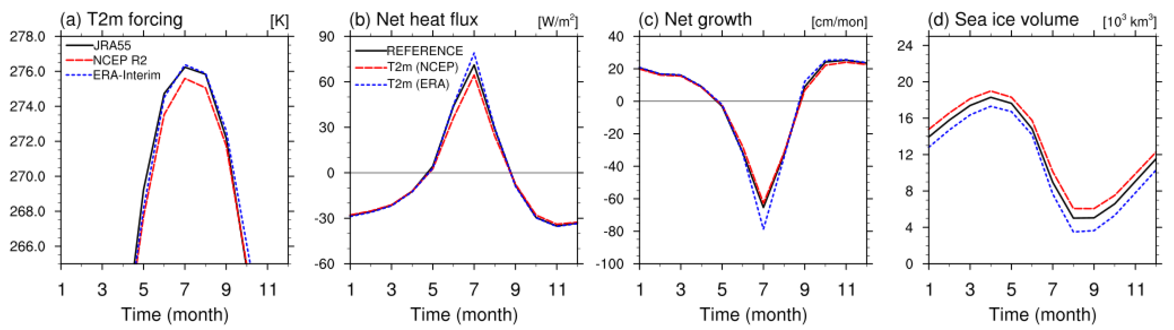
4.2. Sea Ice Response to Temperature Forcing

Except for the radiative forcing experiments, the differences among T2m forcings of the melt season had a relatively large influence on Fnet and the net growth of sea ice. In May, the 2-m temperatures of NCEP R2 and ERA-Interim were approximately 1 K lower than for JRA55 (Figure 1c). This induced lower melt rates than REFERENCE in T2m (NCEP) and T2m (ERA) by decreasing Fnet. In JJA, the temperature forcings of the T2m (NCEP) experiment were as much as 0.8 K lower than that of REFERENCE. In response to these temperature forcings, the total flux over the Arctic of the T2m (NCEP) experiment was smaller than that of REFERENCE by -6 W m−2. In T2m (ERA), although the differences in the 2-m temperature forcings were less than +0.1 K during JJA, a change reaching +3 W m−2 occurred in Fnet. In JJA, the area-averaged 2-m temperature over the Arctic region between ERA-Interim and JRA55 was similar, but the spatial distribution was different. The 2-m temperature for T2m(ERA) was warmer than for REFERENCE over the central Arctic region, and the net heat flux pattern also showed a similar pattern (not shown).
The substitution of temperature forcing changed the Fnet in summer by modifying the FSW and FLW elements as well as the Fsens and Flat in Equation (1) (Figure 5). As a result, the sea ice melted less than in REFERENCE during summer in the T2m (NCEP) experiment and melted more in T2m (ERA). This temperature forcing difference in summer directly caused sea ice volume changes. However, the surface flux and the sea ice growth responses to 2-m temperature forcing changes were not linear in winter. The DJF T2m (ERA) forcings were approximately 0.7 K warmer than those of REFERENCE, but had little effect on Fnet and hence on the net growth (Figure 5c) and sea ice volume (Figure 5d). In September and October, the sea ice growth of T2m (ERA) was slightly faster compared to other experiments (Figure 5c) because the thinner ice (T2m(ERA)) grew faster than thicker ice due to its decreased insulation (the growth-thickness relationship, [40,41]).
The flux difference in these temperature forcing experiments was smaller than that of the radiative forcing experiments, but was still significant. The T2m (NCEP) experiment seemed to have less effect on the average sea ice volume, unlike the LW and SW experiments (Figure 3a). However, in the winter, T2m (NCEP) expressed up to 93% of the sea ice volume variability of PIOMAS, while REFERENCE expressed only 61% (Table 3, Figure S3). This is much larger than the STD of both LW and SW, implying that temperature forcings have a significant influence on the simulation of sea ice volume.

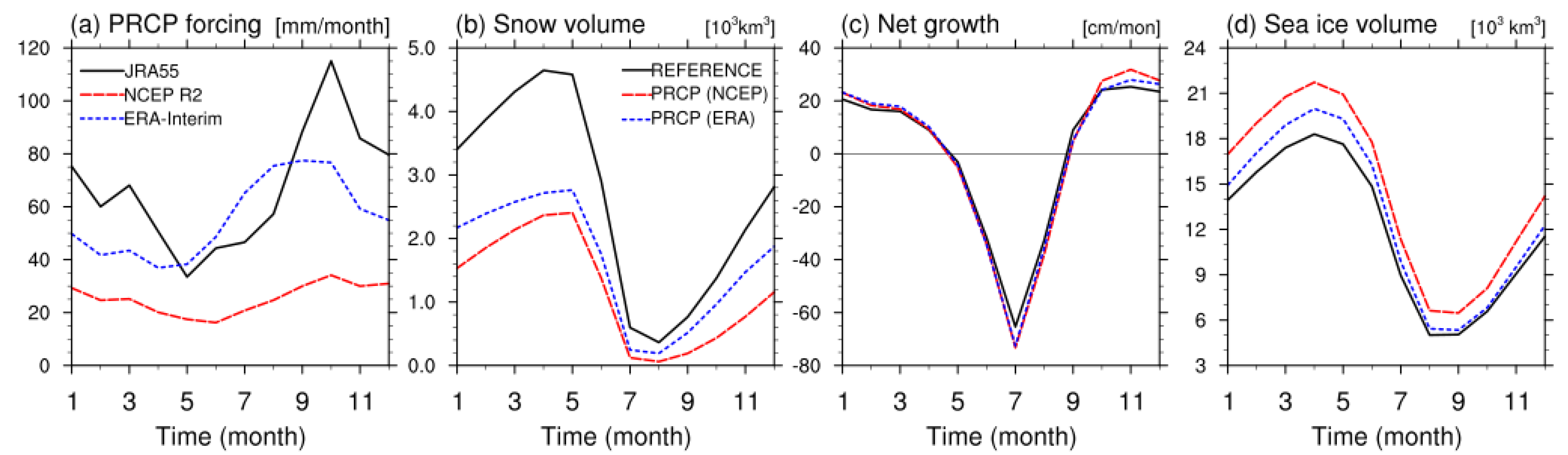
4.3. Sea Ice Response to Hydrological Forcings

Precipitation forcings are a direct source of snow, which serves as an insulator preventing heat exchange between the atmosphere and sea ice. In the PRCP (NCEP) experiment, the precipitation forcings were approximately half those of REFERENCE (Figure 6a). Especially during fall and early winter, when the role of snow depth is most critical in thermodynamic sea ice growth, PRCP forcing of NCEP R2 was just 1/3 that of REFERENCE. Accordingly, the resulting snow volume was approximately half or less that of REFERENCE (Figure 6a,b). The spatial pattern of snowfall rate was different for each reanalysis. During January through March, over the central Arctic, the snowfall for PRCP(NCEP) was slightly more than that for PRCP(ERA), while near the East Greenland Sea and Barents Sea, the snowfall for PRCP(ERA) was much higher than that for PRCP(NCEP). Thus, although NCEP R2 precipitation was less than ERA-Interim, snow volume for PRCP(NCEP) grew faster than PRCP(ERA) (Figure 6a,b). The energy exchange between air and sea ice in PRCP (NCEP) was larger than in REFERENCE because the insulation provided by snow volume was reduced by half. Thus, PRCP (NCEP) produced more ice during the growth period (Figure 6c). Even though the areal averaged net growth rate difference between the two experiments over the whole Arctic was small, there was variability in spatial distribution (not shown). For example, in the central Arctic, the REFERENCE sea ice in June melted faster than that for PRCP (NCEP) at a rate of about 20 cm/month, while in the edge region including the Laptev Sea, sea ice for PRCP(NCEP) melted faster at a rate of about 25 cm/month. Due to this process, the average annual sea ice volume was approximately +22% higher than for REFERENCE.
The precipitation forcing played different roles following the season and the precipitation status. During summer (approximately from May through August), the PRCP(ERA) sea ice volume reduced to a level closer to that of REFERENCE (Figure 6d because the rainfall accelerated the sea ice melt. On the other hand, during winter (approximately from September through April), the PRCP(ERA) sea ice volume increased to a level closer to that of PRCP(NCEP) because thick snow reduced the heat exchange between atmosphere and sea ice.

5. Discussion and Summary

This study compared the uncertainties involved in atmospheric reanalysis data used for atmospheric forcing in sea ice models. We found that discrepancies in the radiative fluxes, surface temperatures, and precipitation among different reanalysis data can cause large uncertainties in sea-ice model simulations. A set of model experiments were conducted by replacing individual forcing variables one by one from a REFERENCE simulation to check the sensitivity of the model with respect to each variable. We found that the CICE5 sea ice model simulated sea ice volume and interannual variability very differently depending on which reanalysis dataset was used for atmospheric forcing. Differences in shortwave radiation in the reanalysis data were the largest of all forcing variables tested; however, the uncertainty measured by the spread of the annual cycle in the simulated sea ice volume was the largest in the substitution experiments for longwave radiation.
Uncertainties in the year-to-year variability were most pronounced for the 2-m air temperature parameter. Among the substitution experiments for T2m, NCEP showed the largest interannual variability. Uncertainty in precipitation forcing affected the amplitude of the sea ice volume annual cycle (PRCP (NCEP)). The insulation effect of the snow seemed to play a key role in sea ice volume changes.
Hunke and Holland [19] applied modified forcing based on Large and Yeager [41] to a global ocean-sea ice model, showing that monthly mean Arctic sea ice extent ranged from 8.5 × 10⁶ km2 to 15.5 × 10⁶ km2 from 1981 to 2000. Notz et al. [14] simulated sea ice using NCEP R1 forcing and ERA-Interim forcing in an ocean-sea ice model from 1979 to 2007; NCEP R1-forced Arctic sea ice extent ranged from 7.9 × 10⁶ km2 to 14.9 × 10⁶ km2 and sea ice volume ranged from 16.5 × 10³ km3 to 34.0 × 10³ km3, while ERA Interim-forced Arctic sea ice extent ranged from 6.7 × 10⁶ km2 to 15.2 × 10⁶ km2 and sea ice volume ranged from 7.2 × 10³ km3 to 25.2 × 10³ km3. In our study, Arctic sea ice extent ranged from 1.5 × 10⁶ km2 to 15.6 × 10⁶ km2 for SW (NCEP) and from 5.5 × 10⁶ km2 to 15.6 × 10⁶ km2 for LW (NCEP), while the Arctic sea ice volume ranged from 1.1 × 10³ km3 to 16.1 × 10³ km3 and from 10.3 × 10³ km3 to 22.1 × 10³ km3, respectively. The Arctic sea ice extent range determined in our study is quite reasonable when compared to the above-mentioned studies, given that previous simulations included the 1980s, when the Arctic sea ice extent was larger. Arctic sea ice volume in our experiments was mostly underestimated.
Identifying a partial component of forcing data that can lead to a sensitive response by sea-ice models is important for the development of improved models and the construction of better observational networks for model use. We used the JRA55 reanalysis as REFERENCE because most of its variables exhibited quantitative value between those of the two other reanalyses (except for precipitation). According to Boisvert et al. [13], the cumulative annual precipitation over the entire Arctic is 519.4 mm for JRA55 and 405.4 mm for NCEP R2. For all our experiments, except PRCP (such as LW(NCEP) or SW(ERA)), we needed to keep in mind that the difference in precipitation forcing between REFERENCE and NCEP R2/ ERA-Interim could influence the experimental results. It seems likely that an experiment in which both LW and PRCP of REFERENCE were replaced by (for example) NCEP R2 forcing would result in a different outcome. However, such experiments were beyond the scope of our study, the main focus of which was to determine to what degree the outcome of a numerical sea-ice model such as CICE5 is sensitive to the atmospheric forcing applied.
In each experiment, the sea ice extent was less sensitive than the sea ice volume and quite similar to that observed by NSIDC. In most experiments, the monthly mean and variations in sea ice volume were underestimated compared to PIOMAS (Table 3 and Figure 3). Thus, further studies should determine how to simulate sea ice volumes more realistically. The errors from the real state may be caused by the effects of atmospheric forcing, as shown in this study, or by the problem of oceanic forcing or physical parametrization [21,42,43,44].
To reduce uncertainty in the reanalysis data, it is necessary to verify these using observed data; however, the Arctic Ocean region is severely lacking in observation points. While observations are relatively dense for land surrounding the Arctic, it is unreasonable to estimate the uncertainty of reanalysis data over the Arctic Ocean using land observations because different uncertainties are included for both areas. For example, the temperature of the ERA-Interim has a cold bias of −0.5 K in the summer around the Arctic [15], and a warm bias up to +2.0 K in the central Arctic [38]. Thus, continuous and dense observations of the Arctic Ocean region should be useful for the sea ice model to reduce simulation uncertainty.
The influence of forcing departures from the true state of sea ice volume varies according to the characteristics of each forcing variable and season. According to Kapsch et al. [39], the perturbations of longwave radiation in summer has a higher influence than those from other seasons. Because the surface temperature in summer is already close to the melting point of ice, small differences in forcings could have large effects on the melting process. In summer, LW(ERA), which is the strongest LW forcing, showed relatively rapid melting compared with other experiments and so reduced the sea ice extent and sea ice volume (Figure 4 and Table 3). In winter, even though the LW forcing of REFERENCE was weaker than the others, corresponding excessive growth was not observed. Moreover, we showed that, in summer, the model is sensitive to shortwave radiation and 2-m temperature forcings. This implies that the summer observation of radiative variables should be a high priority to reduce the uncertainty included in reanalyses. For precipitation forcing, not only precipitation rate and phase of precipitation (rain or snow) but also timing are important. In late spring, rainfall accelerates sea ice melt, while large snowfall delays the onset of sea ice melt [45].

Supplementary Materials

The following are available online at https://www.mdpi.com/2073-4433/10/7/361/s1, Figure S1: Sea ice volume annual cycles in the Arctic region of (a) LW experiments, (b) SW experiments, and (c) T2m experiments, Figure S2: Sea ice volume annual cycles in the Arctic region of replacing experiments, Figure S3: Taylor diagrams of sea ice volumes in the Arctic region.

Author Contributions

S.-B.L. carried out the project, and wrote the paper; B.-M.K. conceptualized the paper, J.U. and J.-B.A. constructively reviewed and edit the paper.

Funding

This research was a part of the project titled ‘Korea-Arctic Ocean Observing System(K-AOOS), KOPRI, 20160245)’, funded by the MOF, Korea.

Conflicts of Interest

The authors declare no conflict of interest.

References

  1. Comiso, J.C. Large Decadal Decline of the Arctic Multiyear Ice Cover. J. Clim. 2012, 25, 1176–1193. [Google Scholar] [CrossRef]
  2. Parkinson, C.L.; DiGirolamo, N.E. New visualizations highlight new information on the contrasting Arctic and Antarctic sea-ice trends since the late 1970s. Remote Sens. Environ. 2016, 183, 198–204. [Google Scholar] [CrossRef] [Green Version]
  3. Onarheim, I.H.; Eldevik, T.; Smedsrud, L.H.; Stroeve, J.C. Seasonal and regional manifestation of Arctic sea ice loss. J. Clim. 2018, 31, 4917–4932. [Google Scholar] [CrossRef]
  4. Stroeve, J.C.; Serreze, M.C.; Holland, M.M.; Kay, J.E.; Malanik, J.; Barrett, A.P. The Arctic’s rapidly shrinking sea ice cover: a research synthesis. Clim. Change 2012, 110, 1005–1027. [Google Scholar] [CrossRef]
  5. Kwok, R.; Cunningham, G.F. Variability of Arctic sea ice thickness and volume from CryoSat-2. Phil. Trans. R. Soc. A 2015, 373, 20140157. [Google Scholar] [CrossRef]
  6. Parkinson, C.L.; Comiso, J.C. On the 2012 record low Arctic sea ice cover: Combined impact of preconditioning and an August storm. Geophys. Res. Lett. 2013, 40, 1356–1361. [Google Scholar] [CrossRef]
  7. Schröder, D.; Feltham, D.L.; Flocco, D.; Tsamados, M. September Arctic sea-ice minimum predicted by spring melt-pond fraction. Nat. Clim. Change 2014, 4, 353–357. [Google Scholar] [CrossRef]
  8. Hunke, E.C.; Bitz, C.M. Age characteristics in multidecadal Arctic sea ice simulation. J. Geophys. Res. Oceans 2009, 114, C08013. [Google Scholar] [CrossRef]
  9. Screen, J.A.; Simmonds, I. Erroneous Arctic temperature trends in the ERA-40 reanalysis: A closer look. J. Clim. 2011, 24, 2620–2627. [Google Scholar] [CrossRef]
  10. Chaudhuri, A.H.; Ponte, R.M.; Nguyen, A.T. A comparison of atmospheric reanalysis products for the Arctic Ocean and implications for uncertainties in air–sea fluxes. J. Clim. 2014, 27, 5411–5421. [Google Scholar] [CrossRef]
  11. Inoue, J.; Yamazaki, A.; Ono, J.; Dethloff, K.; Maturilli, M.; Neuber, R.; Edwards, P.; Yamaguchi, H. Additional Arctic observations improve weather and sea-ice forecasts for the Northern Sea Route. Sci. Rep. 2015, 5, 16868. [Google Scholar] [CrossRef] [PubMed] [Green Version]
  12. Sato, K.; Inoue, J.; Yamazaki, A.; Kim, J.-H.; Maturilli, M.; Dethloff, K.; Hudson, S.R.; Granskog, M.A. Improved forecasts of winter weather extremes over midlatitudes with extra Arctic observations. J. Geophys. Res. Oceans 2017, 122, 775–787. [Google Scholar] [CrossRef] [Green Version]
  13. Boisvert, L.N.; Webster, M.A.; Petty, A.A.; Markus, T.; Bromwich, D.H.; Cullarther, R.I. Intercomparison of precipitation estimates over the Arctic Ocean and its peripheral seas from reanalyses. J. Clim. 2018, 31, 8441–8462. [Google Scholar] [CrossRef]
  14. Notz, D.; Haumann, F.A.; Haak, H.; Jungclaus, J.H.; Marotzke, J. Arctic sea-ice evolution as modeled by Max Planck Institute for meteorology’s Earth system model. J. Adv. Model. Earth, Syst. 2013, 5, 173–194. [Google Scholar] [CrossRef]
  15. Lindsay, R.; Wensnahan, M.; Schweiger, A.; Zhang, J. Evaluation of Seven Different Atmospheric Reanalysis Products in the Arctic. J. Clim. 2014, 27, 2588–2606. [Google Scholar] [CrossRef]
  16. Walsh, J.E.; Chapman, W.L. Arctic cloud-radiation-temperature associations in observational data and atmospheric reanalyses. J. Clim. 1998, 11, 3030–3045. [Google Scholar] [CrossRef]
  17. Makshtas, A.; Atkinson, D.; Kulakov, M.; Shutilin, S.; Krishfield, R.; Proshutinsky, A. Atmospheric forcing validation for modeling the central Arctic. Geophys. Res. Lett. 2007, 34, L20706. [Google Scholar] [CrossRef]
  18. Lüpkes, C.; Vihma, T.; Jakobson, E.; König-Langlo, G.; Tetzlaff, A. Meteorological observations from ship cruises during summer to the central Arctic: A comparison with reanalysis data. Geophys. Res. Lett. 2010, 37, L09810. [Google Scholar] [CrossRef]
  19. Hunke, E.C.; Holland, M.M. Global atmospheric forcing data for Arctic ice-ocean modeling. J. Geophys. Res. 2007, 112, C04S14. [Google Scholar] [CrossRef]
  20. Dumas, J.A.; Flato, G.M.; Weaver, A.J. The impact of varying atmospheric forcing on the thickness of arctic multi-year sea ice. Geophys. Res. Lett. 2003, 30, 1918. [Google Scholar] [CrossRef]
  21. Zhang, J.; Woodgate, R.; Moritz, R. Sea ice response to atmospheric and oceanic forcing in the Bering Sea. J. Phys. Oceanogr. 2010, 40, 1729–1747. [Google Scholar] [CrossRef]
  22. Sturm, M.; Perovich, D.K.; Holmgren, J. Thermal conductivity and heat transfer through the snow on the ice of the Beaufort Sea. J. Geophys. Res. 2002, 107(C21), 8043. [Google Scholar] [CrossRef]
  23. Hunke, E.C.; Lipscomb, W.H.; Turner, A.K.; Jeffery, N.; Elliott, S. CICE: The Los Alamos Sea Ice Model Documentation and Software User’s Manual Version 5.1 LA-CC-06-012; Los Alamos National Laboratory: Santa Fe, NM, USA, 2015; Volume 115.
  24. Wilchinsky, A.V.; Feltham, D. Modelling the rheology of sea ice as a collection of diamond-shaped floes. J. Nonnewton. Fluid Mech. 2006, 138, 22–32. [Google Scholar] [CrossRef]
  25. Turner, A.K.; Hunke, E.C.; Bitz, C.M. Two modes of sea-ice gravity drainage: A parameterization for large-scale modeling. J. Geophys. Res. Oceans 2013, 118, 2279–2294. [Google Scholar] [CrossRef]
  26. Kanamitsu, M.; Ebisuzaki, W.; Woollen, J.; Yang, S.-K.; Hnilo, J.J.; Fiorino, M.; Potter, G.L. NCEP-DOE AMIP-II Reanalysis (R-2). Bull. Am. Meteor. Soc. 2002, 83, 1631–1643. [Google Scholar] [CrossRef]
  27. Dee, D.P.; Uppala, S.M.; Simmons, A.J.; Berrisford, P.; Poli, P.; Kobayashi, S.; Andrae, U.; Balmaseda, M.A.; Balsamo, G.; Bauer, P.; et al. The ERA-Interim reanalysis: Configuration and performance of the data assimilation system. Q. J. R. Meteorol. Soc. 2011, 137, 553–597. [Google Scholar] [CrossRef]
  28. Ebita, A.; Kobayashi, S.; Ota, Y.; Moriya, M.; Kumabe, R.; Onogi, K.; Harada, Y.; Yasui, S.; Miyaoka, K.; Takahashi, K.; et al. The Japanese 55-year Reanalysis “JRA-55”: An interim report. SOLA 2011, 7, 149–152. [Google Scholar] [CrossRef]
  29. Large, W.G.; Yeager, S.G. The global climatology of an interannually varying air-sea flux data set. Clim. Dyn. 2009, 33, 341–364. [Google Scholar] [CrossRef]
  30. Rayner, N.A.; Parker, D.E.; Horton, E.B.; Folland, C.K.; Alexander, L.V.; Rowell, D.P.; Kent, E.C.; Kaplan, A. Global analyses of sea surface temperature, sea ice, and night marine air temperature since the late nineteenth century. J. Geophys. Res. 2003, 108, 4407. [Google Scholar] [CrossRef]
  31. Zhang, J.; Rothrock, D.A. Modelling global sea ice with a thickness and enthalpy distribution model in generalized curvilinear conditions. Mon. Weather Rev. 2003, 131, 845–861. [Google Scholar] [CrossRef]
  32. Fetterer, F.; Knowles, K.; Meier, W.; Savoie, M. Sea Ice Index, Digital Media; National Snow and Ice Data Center: Boulder, CO, USA, 2002. [Google Scholar]
  33. Schweiger, A.; Lindsay, R.; Zhang, J.; Steele, M.; Stern, H.; Kwok, R. Uncertainty in modeled Arctic sea ice volume. J. Geophys. Res. 2011, 116, C00D06. [Google Scholar] [CrossRef]
  34. Lindsay, R.; Haas, C.; Hendricks, S.; Hunkeler, P.; Kurtz, N.; Paden, J.; Panzer, B.; Sonntag, J.G.; Yungel, J.; Zhang, J. Seasonal forecasts of Arctic sea ice initialized with observations of ice thickness. Geophys. Res. Lett. 2012, 39, L21502. [Google Scholar] [CrossRef]
  35. Laxon, S.W.; Giles, K.A.; Ridout, A.L.; Wingham, D.J.; Willatt, R.; Cullen, R.; Kwok, R.; Schweiger, A.; Zhang, J.; Haas, C.; et al. CryoSat-2 estimates of Arctic sea ice thickness and volume. Geophys. Res. Lett. 2013, 40, 732–737. [Google Scholar] [CrossRef] [Green Version]
  36. Stroeve, J.; Barrett, A.; Serreze, M.; Schweiger, A. Using records from submarine, aircraft and satellites to evaluate climate model simulations of Arctic sea ice thickness. Cryosphere 2014, 8, 1839–1854. [Google Scholar] [CrossRef] [Green Version]
  37. Yeager, S.; Danabasoglu, G. The origins of late 20th century variations in the large-scale North Atlantic circulation. J. Clim. 2014, 27, 3222–3247. [Google Scholar] [CrossRef]
  38. Jakobson, E.; Vihma, T.; Palo, T.; Jakobson, L.; Keernik, H.; Jaagus, J. Validation of atmospheric reanalyses over the central Arctic Ocean. Geophys. Res. Lett. 2012, 39, L10802. [Google Scholar] [CrossRef]
  39. Kapsch, M.-L.; Graversen, R.G.; Tjernstorom, M.; Bintanja, R. The effect of downwelling longwave and shortwave radiation on Arctic summer sea ice. J. Clim. 2016, 29, 1143–1159. [Google Scholar] [CrossRef]
  40. Stroeve, J.C.; Schroder, D.; Tsamados, M.; Feltham, D. Warm winter, thin ice? Cryosphere 2018, 12, 1791–1809. [Google Scholar] [CrossRef] [Green Version]
  41. Large, W.G.; Yeager, S.G. Diurnal to decadal global forcing for ocean and sea-ice models: The data sets and climatologies. NCAR Technical Report TN-460+STR 2004, 105. [Google Scholar] [CrossRef]
  42. Björk, G.; Stranne, C.; Borenäs, K. The sensitivity of the Arctic Ocean sea-ice thickness and its dependence on the surface albedo parameterization. J. Clim. 2013, 26, 1355–1370. [Google Scholar] [CrossRef]
  43. Hunke, E.C. Sea ice volume and age: Sensitivity to physical parameterizations and resolution in the CICE sea ice model. Ocean Model. 2014, 82, 45–59. [Google Scholar] [CrossRef]
  44. Hunke, E.C. Weighing the importance of surface forcing on sea ice—A September 2007 modeling study. Q. J. Royal Meteorol. Soc. 2014, 142, 539–545. [Google Scholar] [CrossRef]
  45. Perovich, D.; Polashenski, C.; Arntsenk, A.; Stwertka, C. Anatomy of a late spring snowfall on sea ice. Geophys. Res. Lett. 2017, 44, 2802–2809. [Google Scholar] [CrossRef]
Figure 1. Box plots for average annual cycle (average from 1991 to 2014) of atmospheric variables in the Arctic region (Arctic Ocean north of 65° N) for each reanalysis dataset. (a) SW: Downward shortwave radiation (W m−2); (b) LW: downward longwave radiation (W m−2); (c) T2m: 2-m temperature (K); (d) WIND: wind speed (m s−1); (e) PRCP: precipitation rate (mm month−1); and (f) Q: specific humidity (g kg−1). Black, blue, and red boxes are JRA55, ERA-Interim, and NCEP R2 reanalysis datasets, respectively. The bottom, top, and middle line of each box represent the 25th percentile, 75th percentile, and median, respectively; vertical dashed lines are the range between the min and max values.
Atmosphere 10 00361 g001
Figure 2. Sea ice volume averaged from 1991 to 2014 in the Arctic region, simulated for forcings from the JRA55, ERA-Interim, and NCEP R2 reanalyses, compared with sea ice volume average from PIOMAS. Colored shading define one standard deviation from each simulation.
Atmosphere 10 00361 g002
Figure 3. (a) Sea ice volume and (b) sea ice extent averaged from 1991 to 2014 in the Arctic region for different simulations and data sets. Shading indicates one standard deviation from REFERENCE.
Atmosphere 10 00361 g003
Figure 4. Comparison of the LW experiments. (a) Downward longwave radiative forcing (similar to Figure 1b), (b) net heat flux, (c) net growth rate of sea ice, (d) areal mean of snow and ice surface albedo from the available shortwave radiation, and (e) sea ice volume. The ice surface albedo is shown from March through October because the shortwave radiation is zero for most areas in winter (from November through February). (ce) use the same labels as (b).
Atmosphere 10 00361 g004
Figure 5. Comparison of the T2m experiments. (a) 2-m-temperature forcing (similar to Figure 1c but focused on summer), (b) net heat flux, (c) net growth rate of sea ice, and (d) sea ice volume. (c,d) use the same labels as (b).
Atmosphere 10 00361 g005
Figure 6. Results of the PRCP experiment. (a) Precipitation forcing (similar to Figure 1e), (b) snow volume, (c) net growth rate of sea ice, and (d) sea ice volume. (c,d) use the same labels as (b).
Atmosphere 10 00361 g006
Table 1. Description of the CICE5 model configuration.
ModelCICE5 Stand Alone
Initial conditionNo ice
Atmospheric forcingsMonthly: downward longwave radiation (W m−2), downward shortwave radiation (W m−2), total precipitation rate (kg m−2 s−1)
6 hourly: 2 m air temperature (K), 10 m wind speed (zonal and meridional, m s−1), 2 m specific humidity (kg kg−1), air density (kg m−3)
Oceanic forcingsMonthly HadISST, constant sea surface salinity (34 psu)
DynamicsElastic-Anisotropic-Plastic (EAP)
ThermodynamicsMushy
Integration period1982–2014
Table 2. Description of the CICE5 response experiments for various atmospheric forcings.
EXP NameDescription
REFERENCEAll variables from JRA-55
SW (NCEP or ERA)Same as REFERENCE except downward shortwave radiation from NCEP R2 or ERA-Interim
LW (NCEP or ERA)Same as REFERENCE except downward longwave radiation from NCEP R2 or ERA-Interim
T2m (NCEP or ERA)same as REFERENCE except temperature from NCEP R2 or ERA-Interim
WIND (NCEP or ERA)same as REFERENCE except U and V wind from NCEP R2 or ERA-Interim
PRCP (NCEP or ERA)same as REFERENCE except precipitation from NCEP R2 or ERA-Interim
Q (NCEP or ERA)same as REFERENCE except surface specific humidity from NCEP R2 or ERA-Interim
Table 3. Mean and normalized standard deviations of summer (JJAS) and winter (ONDJFMAM) sea ice volume and sea ice extent.
Sea Ice VolumeSummer (JJAS)Winter (ONDJFMAM)Sea Ice ExtentSummer (JJAS)Winter (ONDJFMAM)
MeanNorm. Std.MeanNorm. Std.MeanNorm. Std.MeanNorm. Std.
PIOMAS12.071.0018.421.00NSIDC8.351.0013.031.00
REFERENCE8.550.5713.840.61REFERENCE7.300.9113.300.93
NCEP*10.970.81*16.290.90NCEP7.730.9713.470.93
ERA6.660.4712.410.48ERA6.921.0513.040.86
SW (NCEP)*4.690.30*11.270.33SW (NCEP)*5.990.9213.230.94
SW (ERA)*11.660.58*16.540.70SW (ERA)7.800.7713.370.92
LW (NCEP)*13.530.72*18.170.86LW (NCEP)*8.210.7913.340.93
LW (ERA)*4.820.35*10.950.39LW (ERA)*6.151.0013.120.96
T2m (NCEP)9.720.8214.780.93T2m (NCEP)7.521.0313.410.94
T2m (ERA)7.390.5512.820.60T2m (ERA)6.991.0213.320.90
WIND (NCEP)8.720.5914.080.62WIND(NCEP)7.330.9113.470.92
WIND(ERA)8.650.5313.780.55WIND(ERA)7.480.9113.170.90
PRCP (NCEP)*10.650.64*16.700.68PRCP (NCEP)7.550.8413.220.90
PRCP (ERA)9.330.5914.910.58PRCP (ERA)7.430.8713.240.90
Q (NCEP)9.290.6414.430.72Q (NCEP)7.450.9213.270.94
Q (ERA)7.820.5713.320.61Q (ERA)7.140.9913.330.92
*Denotes an experiment exceeding one standard deviation of the REFERENCE seasonal mean for sea ice volume (1.78 × 10³ km3 for summer and 1.68 × 10³ km3 for winter) and sea ice extent (0.67 × 10⁶ km2 for summer and 0.38 × 10⁶ km2 for winter).

