Article

Analysis of Mountain Wave Effects on a Hard Landing Incident in Pico Aerodrome Using the AROME Model and Airborne Observations

by
Jin Maruhashi
1,
Pedro Serrão
2 and
Margarida Belo-Pereira
3,4,*
1
Aerospace Group, Instituto Superior Técnico, Lisbon University, 1049-001 Lisboa, Portugal
2
LAETA/CCTAE (Centro de Ciências e Tecnologias Aeronáuticas e Espaciais), Instituto Superior Técnico, Lisbon University, 1049-001 Lisboa, Portugal
3
Aviation Meteorology Division, Portuguese Institute for Sea and Atmosphere, 1749-077 Lisboa, Portugal
4
Centre for the Research and Technology of Agro-Environmental and Biological Sciences (CITAB), University of Trás-os-Montes and Alto Douro, 5001-801 Vila Real, Portugal
*
Author to whom correspondence should be addressed.
Atmosphere 2019, 10(7), 350; https://doi.org/10.3390/atmos10070350
Submission received: 22 May 2019 / Revised: 14 June 2019 / Accepted: 24 June 2019 / Published: 26 June 2019
(This article belongs to the Special Issue Lower Atmosphere Meteorology)

Abstract

:
A hard landing incident in Pico Aerodrome (LPPI) involving an Airbus A320-200 aircraft is investigated using airborne observations and forecasts of the AROME (Applications of Research to Operations at Mesoscale) model. A second flight is also analyzed. The severity of the wind shear during both flights is quantified using the intensity factor “I” that is based on aerial data and recommended by ICAO (International Civil Aviation Organization). During Flight 1, 36% of the landing phase (below 2100 ft) occurred under “severe” wind shear conditions and 16% occurred under “strong” conditions. Upstream characteristics included southwest winds, stable stratification and a Froude number close to 1. According to the AROME model, these circumstances triggered the development of vertically propagating mountain waves, with maximum vertical velocities above 400 ft/min and exceeding 200 ft/min in the flight path. These conditions, together with the severe wind shear, may have caused the incident. During the second flight, a wake with lee vortices and reversed flow developed in the region of the flight path, which is consistent with a low upstream Froude number and/or with the flow regime diagram of previous studies. During the approach phase of this flight, “severe” wind shear conditions were absent, with “strong” ones occurring 4% of the time. It predominantly displayed “light” conditions during 68% of this phase. As a result of the comparison between “I” and the AROME turbulence indicators, preliminary thresholds are proposed for these indexes. Lastly, this study provides an objective verification of AROME wind forecasts, showing a good agreement with airborne observations for wind speeds above 10 kt, but a poor skill for weaker winds.

1. Introduction

In a stably stratified atmosphere, the airflow towards a topographic obstacle may trigger gravity (or buoyancy) waves downstream of the obstacle, known as mountain waves [1]. The flow response to the obstacle depends on several factors like the mountain shape and the Froude number [2]. At a low Froude number, several phenomena have been observed: the flow may be blocked upwind [3] or it may also pass around the obstacle rather than over it (flow splitting phenomenon) [2,4]. In association with the flow splitting phenomenon, a low-level wake may develop on the leeside of the obstacle [4,5,6,7]. The wake can be expressed as a quasi-steady pair of counter-rotating vortices circulating about vertical axes or can present an unstable pattern in which vortices of alternating sign are periodically shed downstream to form a vortex street [4,5]. Also at a low Froude number, wave breaking, indicating the breakdown of laminar flow, may occur above the obstacle [2,4]. On the other hand, at high Froude numbers, airflow will overcome the topographic obstacle and vertically propagating mountain waves may exist depending on the relation between stability, wind and mountain width [8].
The study of such orographic phenomena is of paramount importance in the realm of aeronautics as they have been known to cause a variety of aviation accidents worldwide [9,10] and are especially hazardous to light aircraft during their takeoff and landing phases. Therefore, several authors analyzed aircraft accidents and incidents in various parts of the world, with special attention given to airports or aerodromes directly exposed to orographic flow interference. Aircraft observations have often been compared to NWP (numerical weather prediction) models in an attempt to not only establish their reliability as forecasting tools but to also better comprehend the main causes behind these incidents. Keller et al. [9], for instance, investigated a Continental Airlines aircraft that caught fire after veering violently off of the runway in Denver International Airport (DIA) during takeoff. High-resolution numerical simulations enabled them to conclude that lee waves were the probable cause behind the strong crosswinds that caused the accident. Another study published in 2013 by Parker and Lane [10] revealed that turbulence engendered by orographic flow resulted in a fatal lightweight aircraft accident in Australia.
In Portugal, the behavior of Madeira’s wake has been the subject of several studies [5,11,12]. However, mountain waves associated to Pico Mountain (the highest of Portugal), to the authors’ best knowledge, has only been addressed previously by Barata et al. [13] in a characterization of the surrounding wind regime and validation of the existence of leeside vortices through a scaled physical model of the island placed within a wind tunnel.
Pico Island is one of nine constituents of the Azorean archipelago, situated in the Atlantic Ocean 1500 km from Lisbon (Figure 1). Pico Aerodrome (LPPI) lies on the north coast of the island (Figure S1), north of Pico Mountain with a maximum height of 2351 m (7710 ft). In the presence of southwesterly winds in the southern region of the Island, which are frequent [13], the likelihood that takeoff and landing phases will be affected by a plethora of orographic phenomena ranging from severe mountain waves, leeside vortices and overall LLWS (low-level wind shear) is increased [13,14].
Forecasts of mountain wave induced turbulence rely on algorithms based on outputs of numerical weather prediction (NWP) models. Many of these algorithms rely on wind, temperature and turbulent kinetic energy [15]. Therefore, the accuracy of these fields is a key issue. However, an accurate simulation of such atmospheric variables is particularly challenging in the atmospheric boundary layer (ABL) due to its unsteady and turbulent nature [16]. Several factors may influence the model accuracy, namely, unresolved topographic features [17], turbulence closure schemes [18,19] as well as the representation of turbulence mixing [20,21]. The dynamical core also plays a key role. Ricard et al. [22] for instance, in analyzing the kinetic energy spectra of AROME and Meso-NH models (which have the same physical parameterizations), concluded that a model using a Semi-Implicit Semi-Lagrangian (SISL) scheme has a coarser effective resolution than a model using an Eulerian explicit scheme (less efficient).
The current article focuses on the orographic flow associated to Pico Mountain in two different synoptic backgrounds, using forecasts from the operational AROME (Applications of Research to Operations at Mesoscale) model and airborne measurements collected by SATA (SATA Internacional–Azores Airlines, S.A.) Airbus A320-200 aircraft. Two flights were considered, where the first one represents the hard landing incident (henceforth referred to as Flight 1). Upon touchdown, the aircraft bounced and registered a vertical acceleration above 2 G. No fatalities or serious injuries were reported. The second one, labeled Flight 2, will serve as a control parameter that is representative of a flight in which no incidents were reported.
This study has three goals. The first goal is to characterize the nature of the orographic phenomenon involved during the two flights. The second is to provide an assessment of the agreement between AROME wind forecasts and airborne observations. The third objective is to establish a correspondence between AROME turbulence indicators and the wind shear severity registered by the aircraft. For this purpose, five turbulence indicators (Brown, Ellrod TI1, Ellrod TI2, CAT1 and EDR or Eddy Dissipation Rate) are computed from AROME forecasts. The wind shear perceived by the aircraft is quantified using the wind shear intensity factor “I”, as originally suggested by Woodfield and Woods [23]. This assessment is also of great importance because the Portuguese Institute for Sea and Atmosphere (IPMA) routinely provides AROME forecasts of the wind and EDR for Pico and Faial Islands to SATA on an experimental basis. This test phase started in November 2017.

2. Data and Methodology

This section characterizes the wind from aerial data gathered by SATA A320-200 aircraft during both flights. The method of calculation of the wind shear intensity factor “I”, which is a function of these airborne measurements, is established. A brief description of the AROME model is also provided. The Froude number and turbulence indicators, which are based on forecasts, are then defined. Lastly, definitions for the RMSE (root mean square error) and MAE (mean absolute error) concerning wind magnitude and direction are included.

2.1. SATA Airborne Measurements
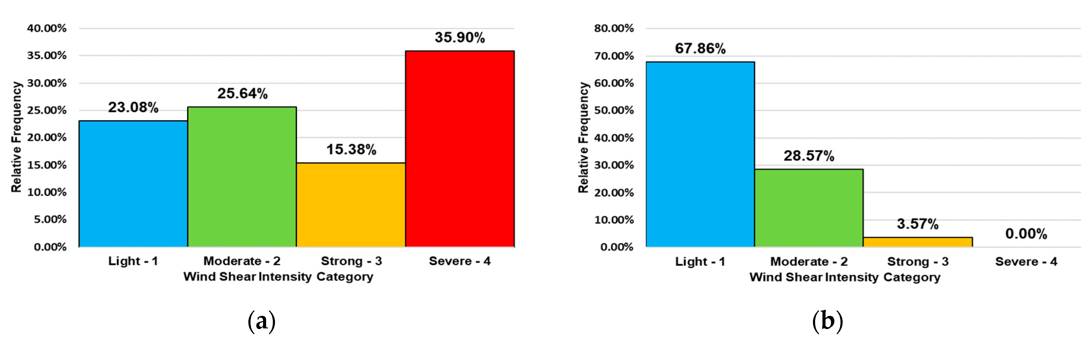
For each flight, wind intensity and direction were recorded approximately every 4 s along with the corresponding altitude and geographical coordinates (latitude and longitude). Only the approach and landing phases (approximately final 10 min of flight or altitudes below 5000 ft) were perused since these are the most pertinent to understanding the incident. The average trajectory for both flights along with Pico’s orography in the AROME model are mapped in Figure 2.

2.2. Wind Shear Intensity Factor “I

The severity of wind shear intensity, as perceived by the aircraft, will be measured according to the wind shear intensity factor “I”, detailed in ICAO’s (International Civil Aviation Organization) Manual on Low-level Wind Shear [24]. Following Guan and Yong’s study [25], wind shear is classified as “light”, “moderate”, “strong” or “severe” based on the variation of the airspeed with time d V T A S d t and on the airspeed proportion Δ V T A S V T A S . The intensity factor “I” itself may be expressed as follows:
I = d V T A S d t · ( Δ V T A S V T A S ) 2
The computation of the true airspeed, V T A S , is based on the following relation:
G S = V T A S + V H T ,
where G S represents the ground speed of the aircraft and was computed by employing the three-dimensional distance formula between any two points described by their altitude and geographic coordinates (latitude and longitude). Note that Δ V T A S is simply the difference between true airspeeds at the n th and ( n + 1 ) th instants. The head or tailwind component (see Equation S2.1 and Figure S2, from Supplementary Materials) is then subtracted from the ground speed to obtain the true airspeed.
Once d V T A S d t and Δ V T A S V T A S are known, the wind shear intensity may be classified by consulting the proper boundaries specified in Figure S3 from the Supplementary Materials. In both flights, this was performed for altitudes approximately below 2000 ft (610 m), which according to Guan and Yong [25], represents the appropriate range for low-level wind shear considerations.

2.3. Description of the AROME Model

The AROME model that runs operationally at IPMA uses a horizontal grid spacing of 2.5 km. It uses a SISL scheme and employs a three-class ice scheme with ECMWF (European Center for Medium-Range Weather Forecasts) radiation parameterizations, as was described by Seity et al. [26]. The representation of turbulence in the ABL is based on a prognostic TKE (Turbulent Kinetic Energy) equation [27], combined with a diagnostic mixing length. AROME initial and boundary conditions emanate from the ARPEGE (Action de Recherche Petite Échelle Grande Échelle) model. At the time of Flight 1, the operational AROME model was integrated with 46 levels, while at the time of Flight 2, additional vertical levels were incorporated, leading to a total of 60 levels.

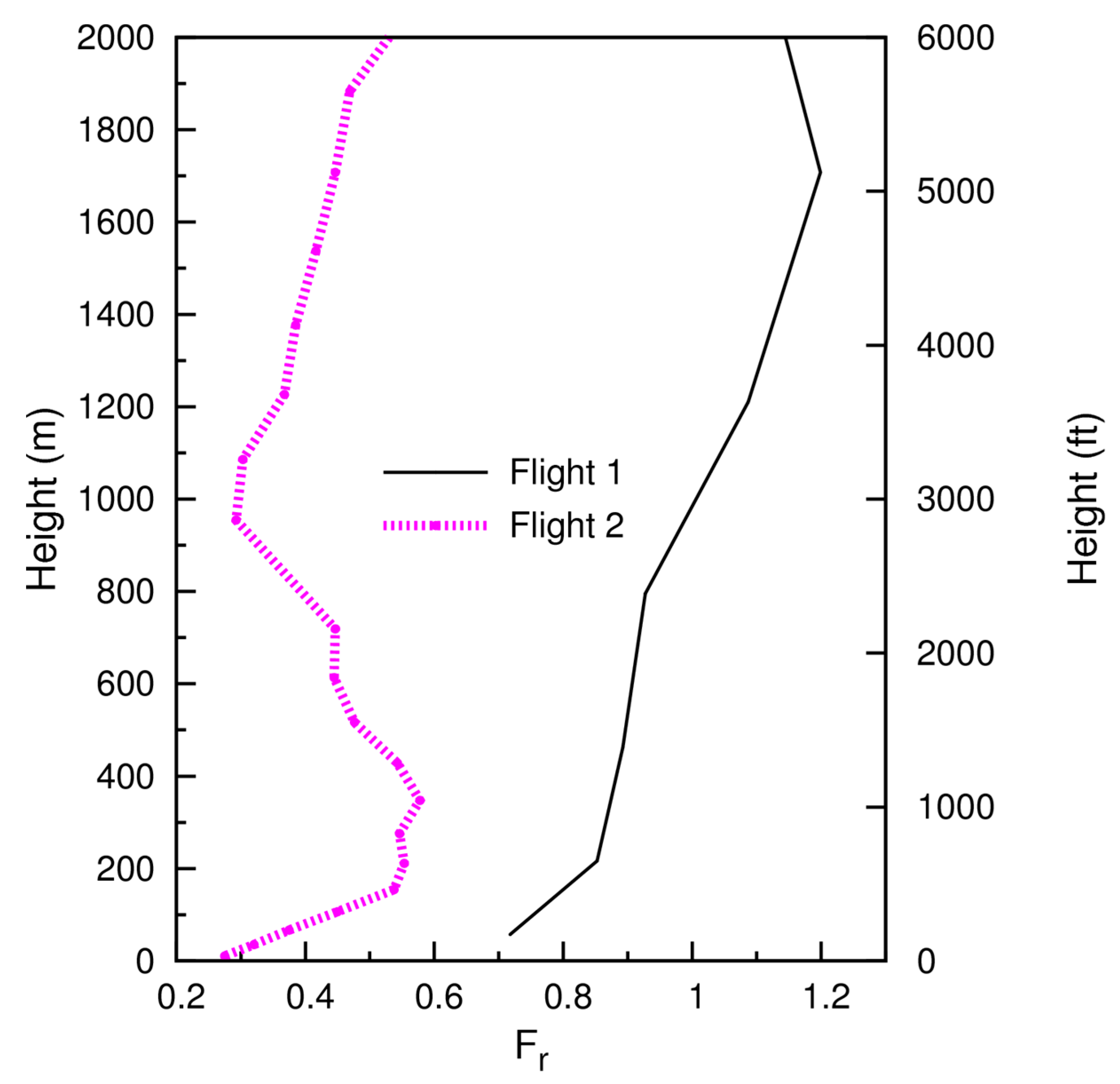
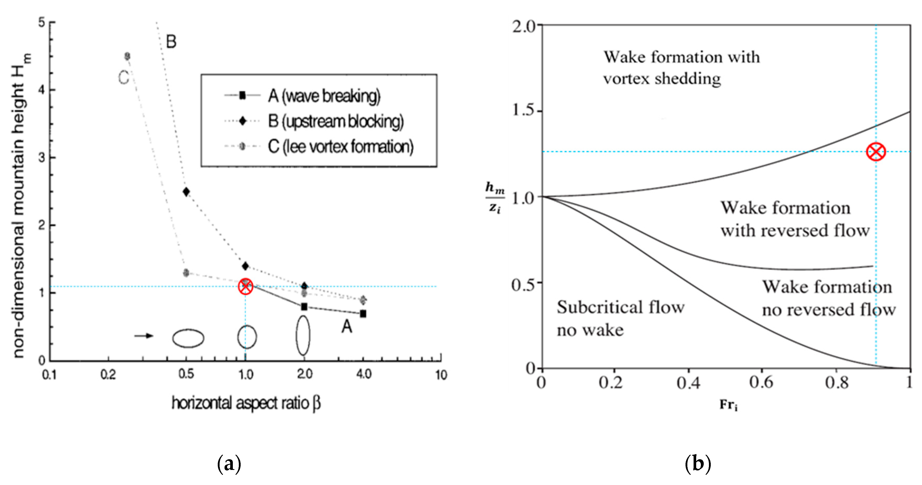
2.4. Froude Number Definitions

The Froude number is a dimensionless parameter that may be utilized to describe the interaction mechanism between kinetic and potential energies as air flows past orography, according to Sutherland [28]. The Froude number can be interpreted as the ratio of the inertial to gravity forces in the flow (Lynch and Cassano [29]). This ratio may also be interpreted physically as the ratio between the mean flow velocity and the shallow water gravity wave speed (Holton [30]). The Froude number has also been applied to infer the type of flow phenomenon that may occur in the lee of a mountain when paired with a flow regime diagram, as was done by Sheridan and Vosper [31].
Three definitions of the Froude number were considered in this study. The first is the classical form, the second is based on Sheppard’s dividing-streamline concept [32] and the third is applicable when a temperature inversion is present in the vicinity of the upstream region of the mountain. The exact upstream location at which Froude numbers were computed in both flights is indicated by point C in Figure 2.

2.4.1. Classical Froude Number, Fr

The classical Froude number, Fr , may be defined as:
Fr = U ¯ N h m ,
where U ¯ is upstream flow speed, N is the Brunt-Väisälä frequency and h m is the mountain height [6,7,33]. Vosper et al. [34] provide an additional definition, F L , that is based on a horizontal length scale L , such that F L = U / N L . In this study, h m is 1200 m, which is the maximum height of Pico Mountain according to AROME topography and L = 21 km. Some authors [2,4,35], alternatively, refer to the non-dimensional mountain height M as:
M = 1 Fr = N h m U n m ,
where N would now represent an average value for the Brunt-Väisälä frequency below h m and U n m a cross-mountain wind speed average also under h m , as is done similarly by Jiang et al. [35].
Several authors summarize their results from laboratory, numerical and theoretical studies in a schematic regime diagram showing that for Fr > 1 mostly small-amplitude gravity waves are expected, while for Fr < 1 , flow splitting, lee vortices and/or wave breaking may occur depending also on the horizontal aspect ratio of the obstacle. This is seen in Figure 2 from [4] and in Figure 13 from [2], the latter of which is shown here as Figure A1a.
For the parameter F L , whenever F L 1 vertically propagating waves are expected, but are evanescent if F L > 1 [34].

2.4.2. Froude Number ( Fr h ) in Terms of the Dividing-Streamline Height h c

Under stable conditions and with varying wind speed and stratification, according to Sheppard [32] and Heinze et al. [6], it is possible to determine the dividing-streamline height h c (also called the critical height) as follows:
1 2 V ¯ h 2 ( h c ) = h c h m N 2 ( z ) ( h m z ) d z ,
where Heinze et al. [6] define V ¯ h as the mean horizontal velocity as a function of the horizontal velocity components u and v : V h = u 2 + v 2 . It is assumed in Equation (5) that all the kinetic energy of the flow is converted into potential energy [6]. As was done in [6], Equation (5) will be solved iteratively for h c via the trapezoidal rule to numerically compute the integral.
As noted by Heinze et al. [6], if Fr > 1 , all fluid parcels, even near the surface, can flow over the obstacle. On the other hand, when Fr < 1 , the fluid may stagnate in the upstream region below a certain critical height h c , passing primarily around the orographic obstacle rather than over it (flow splitting phenomenon). Above h c , the flow would be able to ascend the obstacle [6]. An illustration of flow splitting and of the critical height h c is provided in Figure 3.
So, when flow splitting occurs, an expression for the Froude number in terms of the dividing-streamline height may then be obtained, as is noted by Trombetti and Tampieri [36]:
Fr h = 1 h c h m .
According to Wooldridge et al. [37], Equation (6) may also be used to find the critical height h c if Fr h is replaced by Fr (defined by Equation (3)), which is applicable when Fr < 1 .

2.4.3. Inversion Froude Number ( Fr i )

The inversion Froude number may be computed in the presence of an inversion by adopting Vosper’s [38] definition:
Fr i = U n m g z i ,     g = g θ θ m .
where z i is the inversion height, θ is the magnitude of the potential temperature difference across the inversion, θ m is the mean potential temperature below the inversion base and U n m is the cross-mountain wind speed (averaged below z i ). See Figure 3 for a visual representation of some of these parameters.
In the presence of a temperature inversion, several authors [5,38,39] provide a regime diagram for a two-layer flow over mountains as a function of the inversion Froude number (Equation (7)) and of the ratio h m z i , as is shown in Figure A1b from Appendix A.

2.5. Turbulence Indicators

Five turbulence indicators commonly used in aviation meteorology applications [40,41] are used in this study: Brown, Ellrod TI1, Ellrod TI2, CAT1 and EDR. These parameters were calculated using AROME forecasts.

2.5.1. Brown Index Φ

According to Gill and Buchanan [40] and Sharman et al. [41], the Brown Index Φ may be defined as:
Φ = 0.3 ζ a 2 + ( v x + u y ) 2 + ( u x v y ) 2 ,     ζ a = ( v x u y ) + f
with u and v denoting the zonal and meridional components of the wind respectively. The vertical component of the absolute vorticity is represented by ζ a , which is the sum of the vertical component of the relative vorticity and the Coriolis frequency f .
The form applied in this work, Φ ε , was based on Equation (8) and is expressed as energy dissipation in the following manner:
Φ ε = 1 24 Φ S V 2 ,     S V = ( u z ) 2 + ( v z ) 2
where S V is the vertical wind shear.

2.5.2. Ellrod TI Indexes

As is mentioned in [40], the Ellrod indicators can be used to quantify turbulence. The first version, Ellrod TI1, is defined as:
Ellrod   TI 1 =   S v ( u x v y ) 2 + ( v x + u y ) 2 ,
where S v is the vertical wind shear. The Ellrod TI2 index is similar to the Ellrod TI1, except that it incorporates a convergence term in the form of ( u x + v y ) , as is shown in Equation (11):
Ellrod   TI 2 = S v [ ( u x v y ) 2 + ( v x + u y ) 2 ( u x + v y ) ] .

2.5.3. CAT1 Indicator

The CAT1 turbulence indicator, as is denoted in this study, is referred to as “MOS (Model Output Statistics) probability forecast” by Sharman et al. [41] and is defined as:
CAT 1 = V h ( u x v y ) 2 + ( v x + u y ) 2 ,
where V h is the horizontal wind speed.

2.5.4. EDR Indicator

The Eddy Dissipation Rate, ε , may also be used as a quantifier for turbulence. The method of calculation for this parameter in the current study followed the empirical formula delineated in Frech et al. [42]:
ε = TKE 1.5 L e ,
where L e = 311 m, which is the chosen length scale [42]. TKE represents the turbulent kinetic energy, which is a prognostic variable from the AROME model. The EDR indicator itself, however, was defined as the cube root of ε according to ICAO [43]:
EDR = ε 1 3 .
This study presents EDR because it is the standard measure to quantify turbulence in aviation applications. Nevertheless, for other scientific communities, it is relevant to show TKE forecasts, which are presented in the supplementary materials.

2.6. RMSE and MAE for Wind Speed and Direction

The quantitative comparison between observed (from aircraft) and forecast (from AROME) wind data is established using the root mean square error (RMSE) and the mean absolute error (MAE). The calculation of the wind speed error, RMSE WSPD , is performed following the method employed by Grubišić et al. [5] for a dataset with n points, as follows:
RMSE WSPD = 1 n i = 1 n [ V h ( i ) o b s V h ( i ) s i m ] 2 .
MAE WSPD is similarly defined as follows:
MAE WSPD = 1 n i = 1 n | V h ( i ) o b s V h ( i ) s i m | .
The root mean square error and the mean absolute error for the wind direction, RMSE WDIR and MAE WDIR respectively, are determined using the method described in Jiménez et al. [44]:
RMSE WDIR = 1 n i = 1 n [ Δ WDIR ( i ) ] 2 ,
MAE WDIR = 1 n i = 1 n | Δ WDIR ( i ) | ,
where Δ WDIR ( i ) in degrees is given by:
Δ WDIR ( i )   = { WDIR s i m ( i ) WDIR o b s ( i ) ; | WDIR s i m ( i ) WDIR o b s ( i ) | 180 WDIR s i m ( i ) WDIR o b s ( i ) 360 ; WDIR s i m ( i ) WDIR o b s ( i ) > 180 WDIR s i m ( i ) WDIR o b s ( i ) + 360 ; WDIR s i m ( i ) WDIR o b s ( i ) < 180 .
The comparison between model and observation was done according to the following two-step approach in order to find corresponding values for a given airborne observation:
  • The absolute difference between all AROME levels for each recorded flight altitude, expressed as | Altitude Flight Altitude AROME | , is computed and the level with the minimum difference is selected as the best match. This process is repeated for each available flight altitude.
  • Once every flight altitude is paired with an AROME level, a latitude and longitude pair must be chosen at each one of these correspondences. Following a similar logic, the best coordinate pair from the model was deemed to minimize the distance relative to the flight coordinates at each altitude.

3. Results and Discussion

This section begins by illustrating results based on aerial observations. The wind shear intensity factor “I” is then analyzed. Next, outcomes based primarily on AROME forecasts like Froude numbers and turbulence indicators are discussed. Finally, the accuracy of AROME wind predictions is assessed by comparing them with data that was collected by SATA aircraft, using objective scores.

3.1. Observations

3.1.1. Aerodrome Wind Data

At the LPPI aerodrome, wind was predominantly from the southwest at two instants close to the time of both flights (Table 1). A headwind ( W H D ) of 12/13 kt (6/7 ms−1) and a crosswind ( W C H ) of 14/16 kt (7/8 ms−1) were registered on the day of Flight 1. In regard to gusts, the aircraft experienced a headwind ( G W H D ) of 18/20 kt (9/10 ms−1) and a crosswind ( G W C H ) of 21/24 kt (11/12 ms−1) incoming from the left.

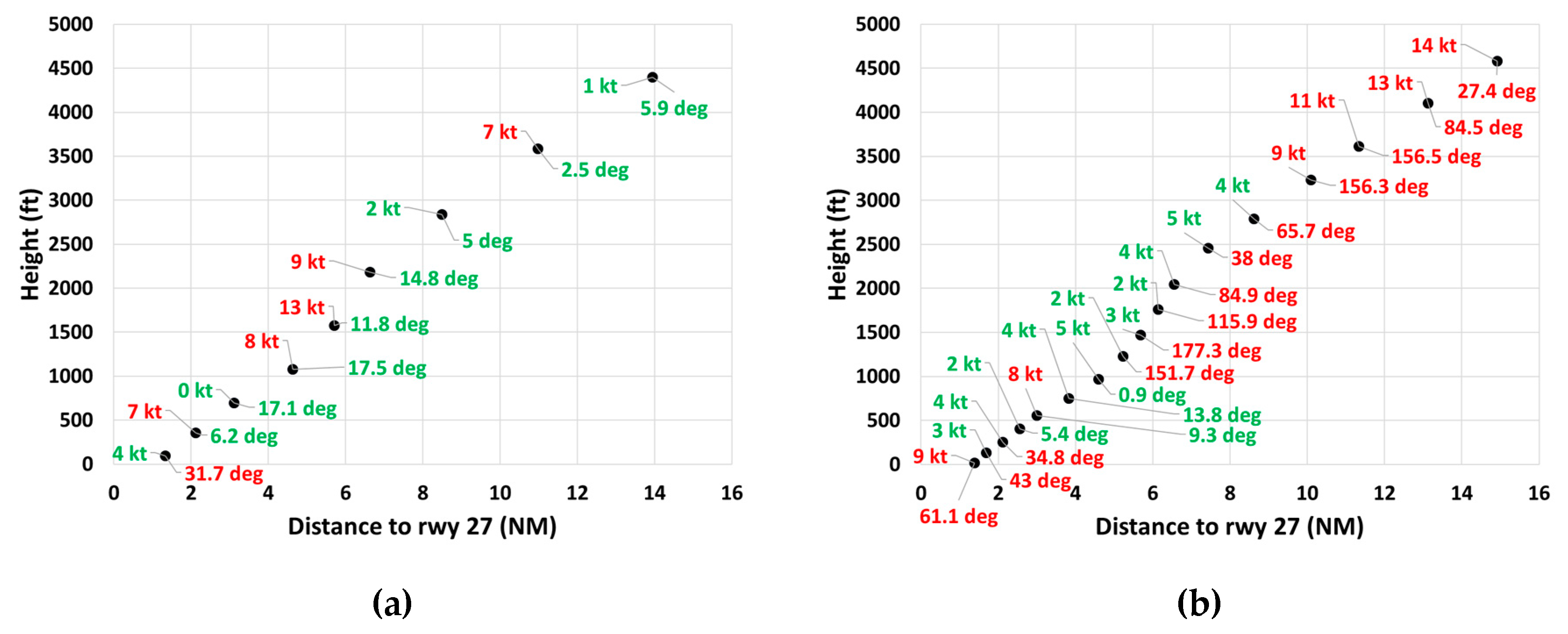
3.1.2. Characterization of Wind Profiles

The wind speed profile based on airborne observations along its path (see Figure 2 and Figure S1) is presented in Figure 4, for Flights 1 and 2. During Flight 1, the aircraft experienced strong winds oscillating between 10 kt (5 ms−1) and nearly 40 kt (21 ms−1). At 440 ft (107 m), for instance, the aircraft experienced a wind of 38 kt (19.5 ms−1). During Flight 2, in the approach phase, the wind speed reaches its maximum of nearly 22 kt (11 ms−1) at 600 ft (183 m), at a distance of 1.67 NM of the aerodrome. Closer to the aerodrome, the wind decreases to 5 kt (3 ms−1) near the surface. Above 1000 ft (305 m) at a distance of nearly 4 NM of the aerodrome, the wind is weak (below 8 kt or 4 ms), due to the wake in the lee of Pico Mountain, as will be shown in the next sections. During both flights, the wind was predominantly from the southwest below 1500 ft or 457 m (Figure S4).

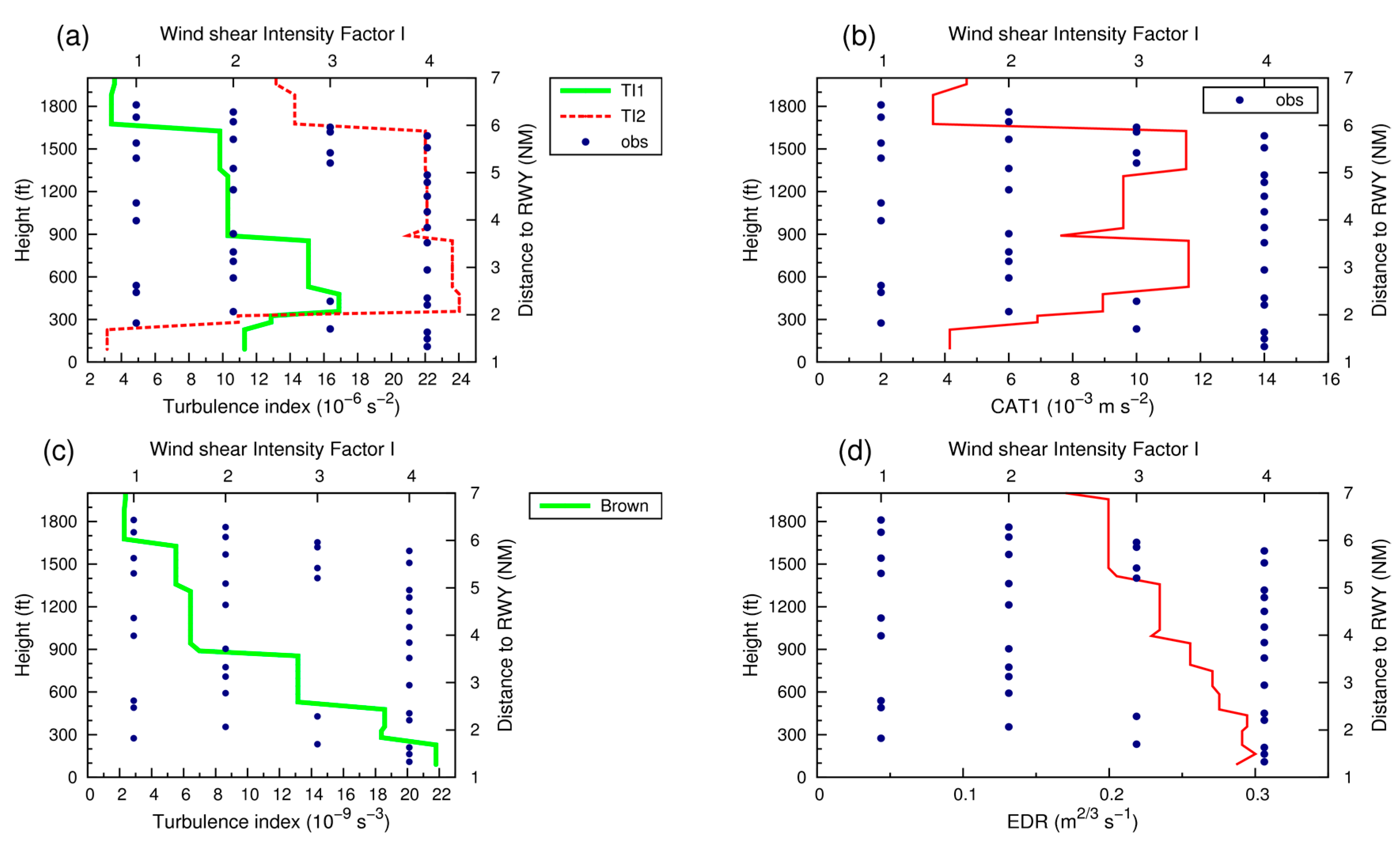
3.1.3. Wind Shear Intensity Factor “I”

Figure 5a,b detail the relative frequency distributions in both flights for altitudes only below 2100 ft (640 m) in order to focus on the effects of low-level wind shear as is suggested in [25]. During Flight 1, about 36% of the approach phase was carried out under “severe” wind shear conditions and over 15% under “strong”. In other words, more than 50% of it experienced “strong” to “severe” wind shear, which is consistent with the occurrence of the hard landing incident. During Flight 2, “severe” wind shear conditions were absent, with only 4% being classified as “strong” and nearly 29% as “moderate” (Figure 5b). Table 2 lists wind shear levels of the first three lowest levels as functions of d V d t and V V for both flights. By comparing them, it is clear that within the three closest levels to the ground, the hard landing incident (Flight 1) exclusively experiences “severe” wind shear, whereas in Flight 2, a “light” intensity is prevalent.

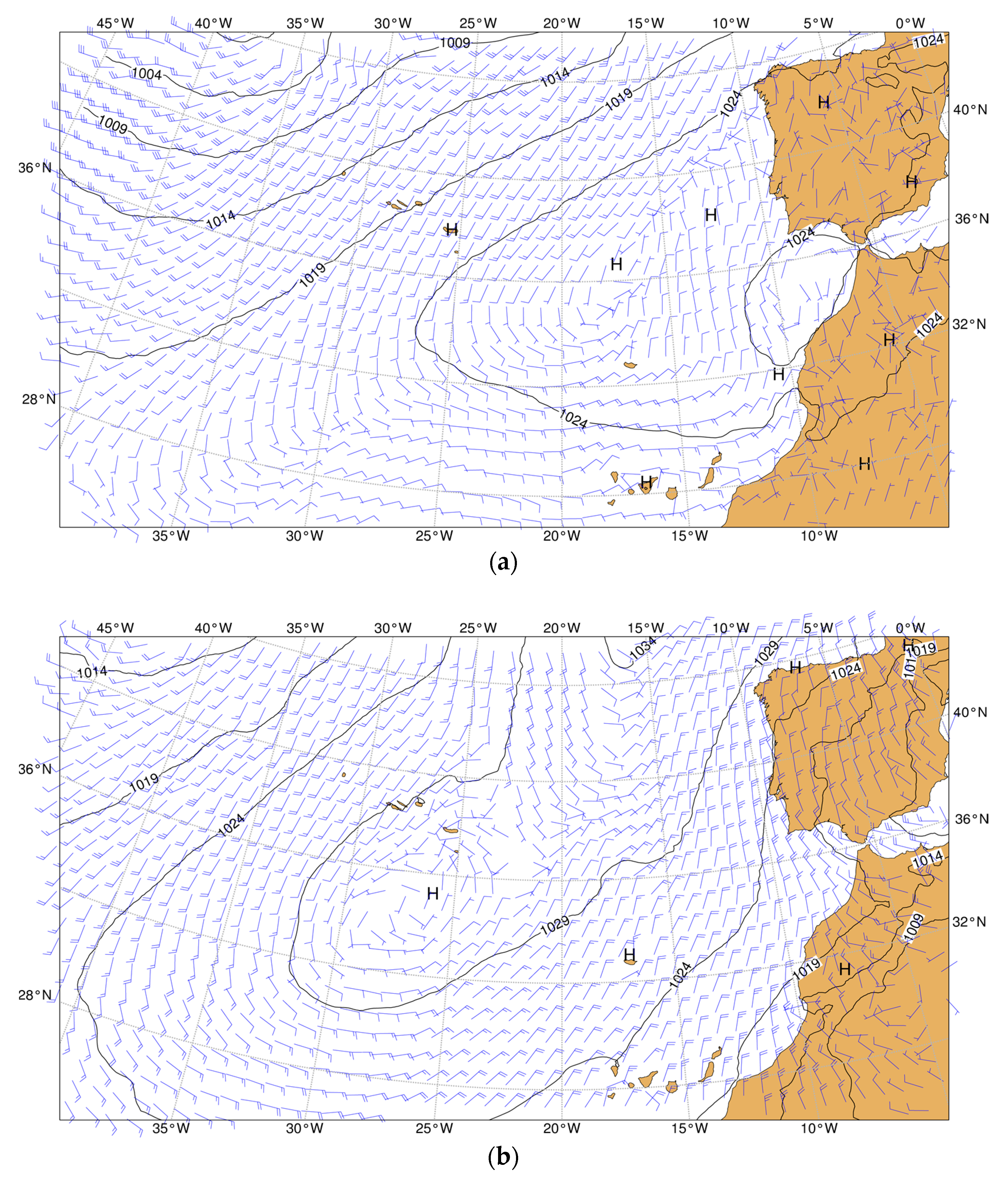
3.2. Synoptic Analysis

During Flight 1, the flow in Pico Island was influenced by the presence of a depression located northwest of the Azores and by a subtropical anticyclone to its west/southeast. Consequently, southwesterly winds of around 20 kt (10 ms−1) were visible south of the island, according to an ECMWF analysis (Figure 6a). For Flight 2, an anticyclone was present south of the Azores, causing southwesterly winds of approximately 10 kt (5 ms−1) south of Pico Island (Figure 6b).

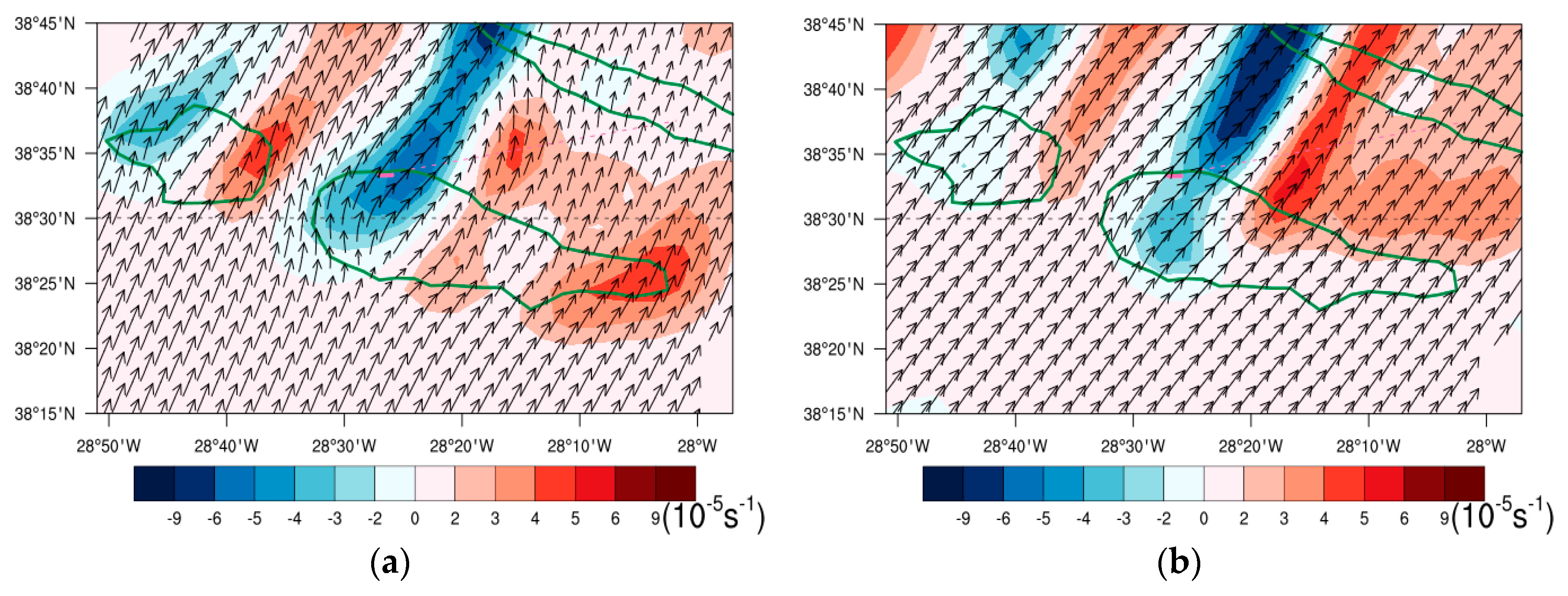
3.3. Mesoscale Analysis

During Flight 1, according to AROME forecasts, the upstream conditions are characterized by a stable stratification, with N varying from 0.012 to 0.015 s−1 and by the absence of an inversion (Figure S5a). The Froude number varies between 0.7 and 0.9 below 400 m, reaching a maximum value of 1.2 at about 1600 m (Figure 7), which coincides with a wind speed of nearly 18 ms−1 (Figure S5c). Above this level, F r varies between 1 and 1.2. Consistently, F r and F r h are 0.95 and 0.9, respectively (Table 3). Therefore, according to previous studies [2,4], no wave breaking, upstream blocking or lee vortex formation are expected (see Figure A1a). The critical height defined in Section 2 is 107 m or 60 m, depending on the method. Consequently, it is expected that air will flow nearly horizontally around the mountain below this level, but will overcome the obstacle above it. Moreover, the parameter F L is always below 0.08 (Figure S5c) and so, according to the analysis of F L and the Froude number, vertically propagating waves are expected [34].
During Flight 2, the upstream conditions are characterized by the presence of a short inversion close to 3000 ft (872 m), where N varies between 0.015 and 0.018 s−1 (Figure S5b). The Froude number has values smaller than 0.6 below 2 km (Figure 7). Consistently, F r and F r h are 0.42 and 0.31, respectively (Table 3). According to the flow regime diagram presented in Figure A1b, flow splitting and lee vortex formation with reversed flow are expected.

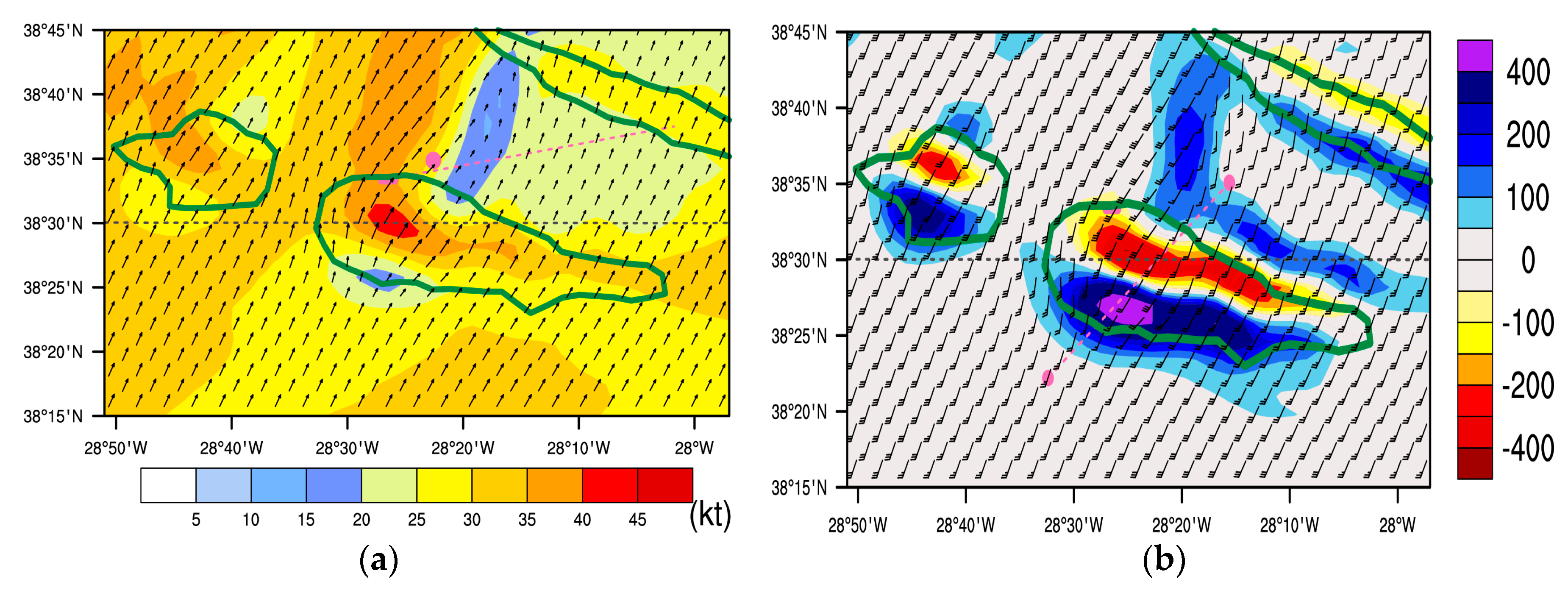
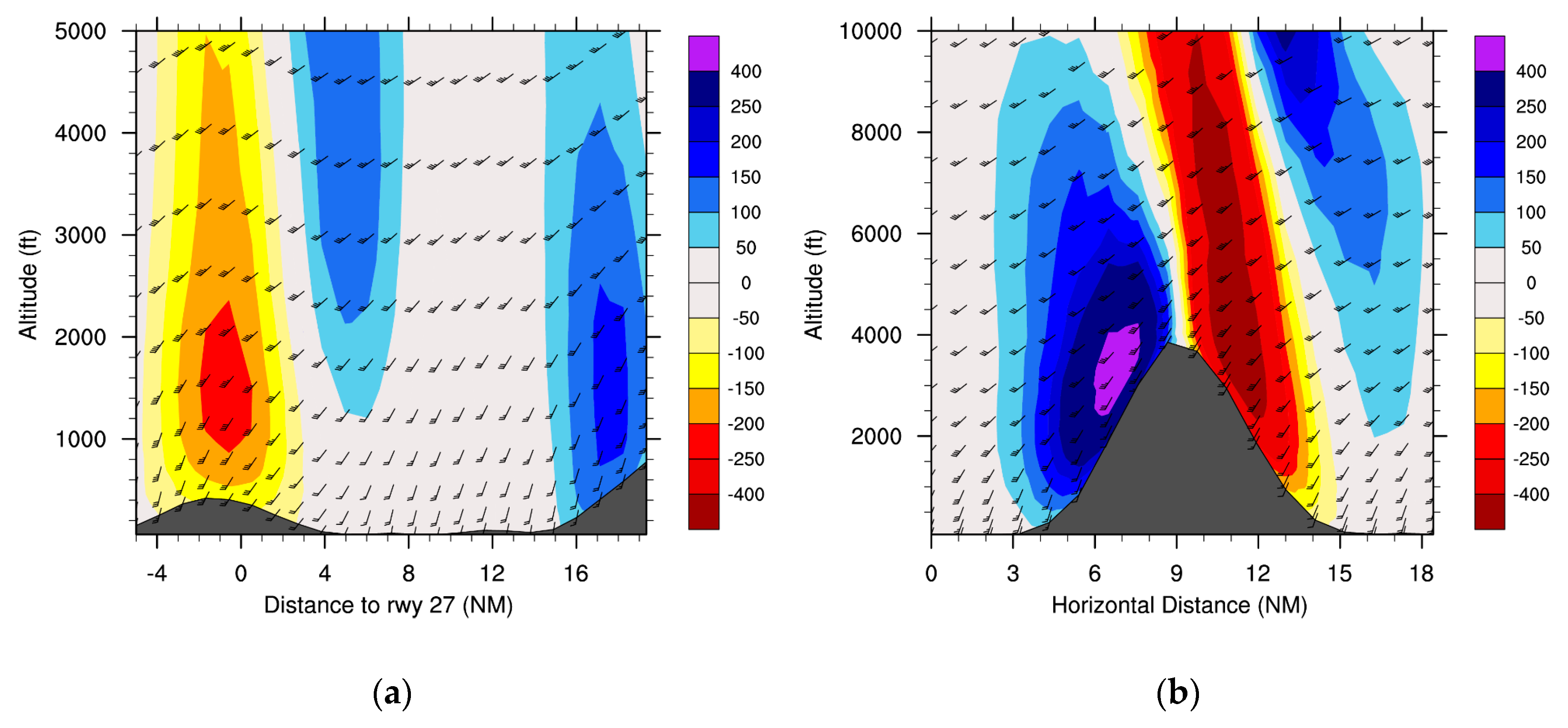
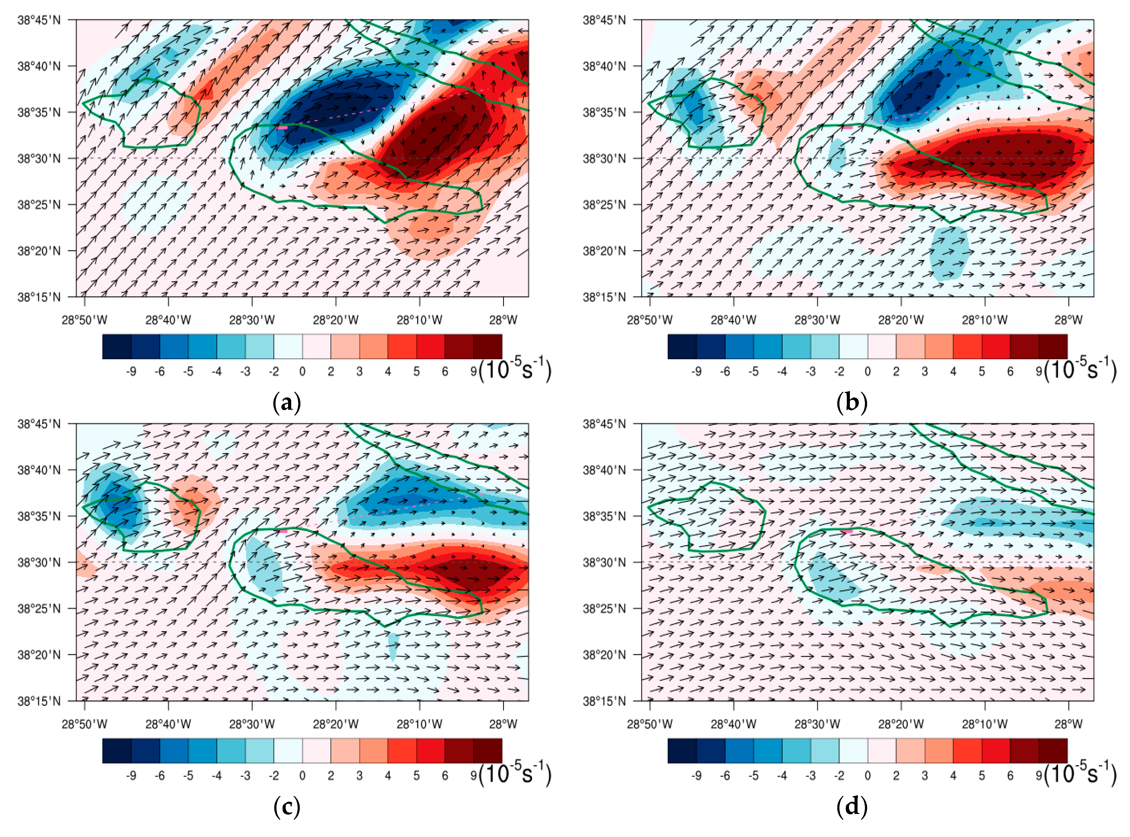
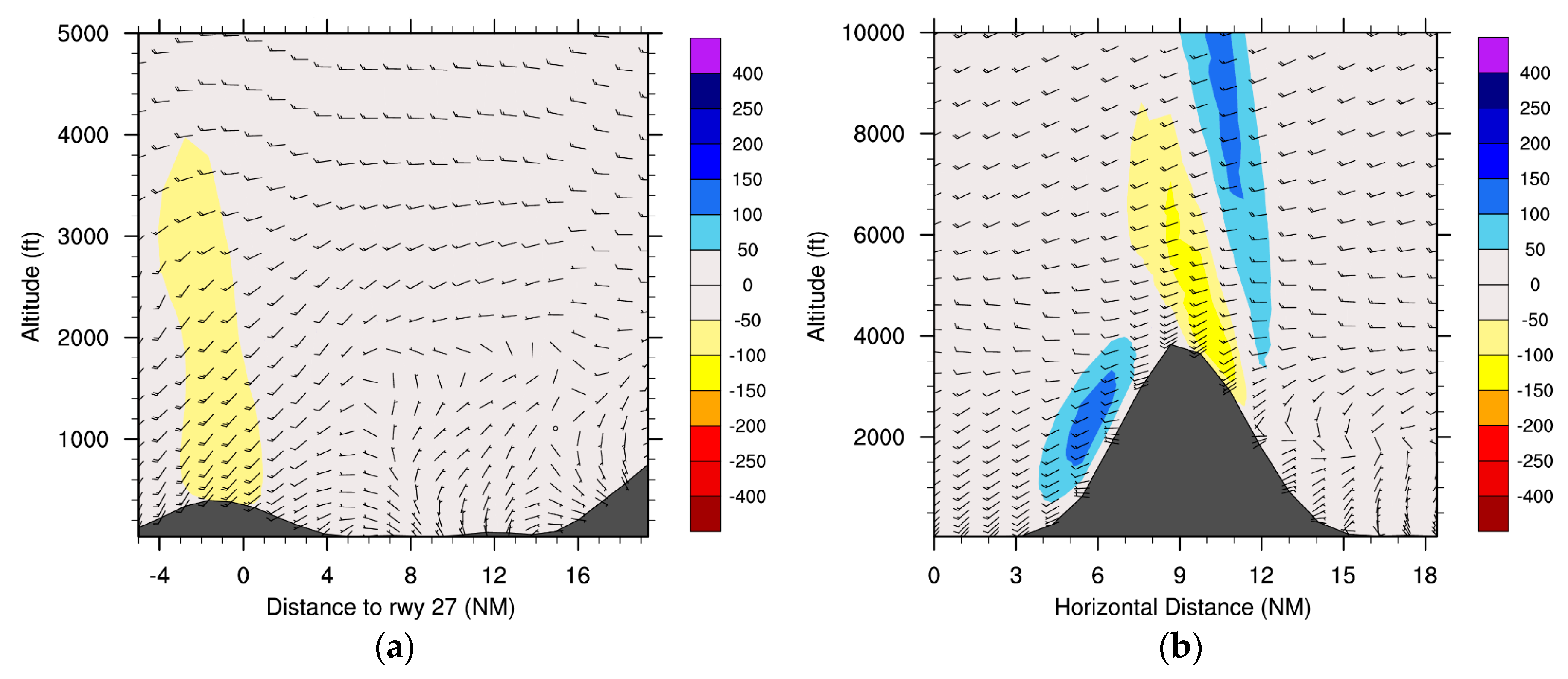
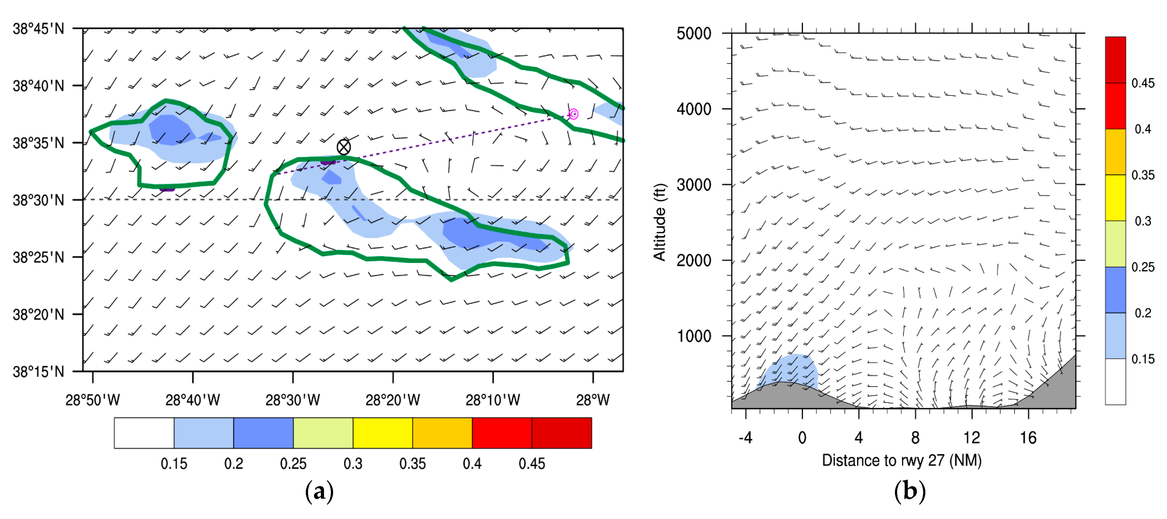
3.3.1. Characterization of Orographic Flow during Flight 1

The horizontal wind and vertical component of the absolute vorticity predicted by the AROME model are depicted in Figure 8 for Flight 1. At 30 m, the flow is partially deflected laterally (mostly on the west side), which is denounced by the curvature of the wind vectors. This deflection is still present at 200 m but is barely visible at 300 m (not shown), while at 500 m (Figure 8b) it is no longer discernible at all. This implies that the critical altitude ( h c ) should lie somewhere between 200 and 300 m. From Table 3, it may be seen that h c 1 = 107 m and h c 2 = 60 m, revealing that the estimate based on Equation (5) is more accurate. However, it underestimates h c , possibly due to an insufficient vertical resolution of the AROME model.
Until 2800 ft (853 m), a pair of positive and negative vertical vorticities is visible over the mountain and on the leeward region, illustrated in Figure 8a for a height of 30 m. However, no signs of reversed flow or vortex formation are present, which is consistent with the results of Bauer et al. [2] and Epifanio [4].
The horizontal wind speed at 680 ft (207 m) shows a stagnation area on the upstream region of Pico Mountain and a maximum wind speed (>40 kt or 21 ms−1) over it with weak winds on the leeward side (Figure 9a). This pattern is coherent with previous studies like in Bauer et al. [2] with their Figure 2.a2. Near Pico Aerodrome, AROME forecast winds with speeds above 35 kt (18 ms−1). Ergo, during the approach to the aerodrome, the aircraft passes a region of elevated wind shear. Figure 9b presents the maximum and minimum vertical velocities in the layer from the surface up to 6000 ft (1829 m), illustrating a wave pattern over Pico and Faial Islands. Figure 10a displays the vertical cross-section through the flight path in the approach phase (line A–B in Figure 2), showing that AROME forecasts the upward vertical velocity in the order of 100 ft/min (0.5 ms−1) near 2000 ft (610 m) and a downward vertical velocity of 100–150 ft/min (0.50–0.76 ms−1) near the aerodrome. This is associated with pronounced vertically propagating waves, which are illustrated in Figure 10b (up to 10000 ft or 3048 m) and in Figure S6a (up to 42000 ft or 12802 m), where the highest values exceed 400 ft/min (2 ms−1), and then propagate to the vicinity of the aerodrome.
During Flight 1, the mean wind speed at point C (from Figure 2) is 12.76 ms−1 ( U ) and the average value of the buoyancy frequency is 0.0129 s−1 ( N ). Since the horizontal scale ( L ) for Pico Mountain is of the order of 21 km, the condition for vertically propagating gravity waves ( N 2 > U 2 k 2 ) applies [1,29]. See also Figure 13.3 in Cassano and Lynch [29], which illustrates the alternating pattern between upward and downward motion associated with vertically propagating gravity waves.

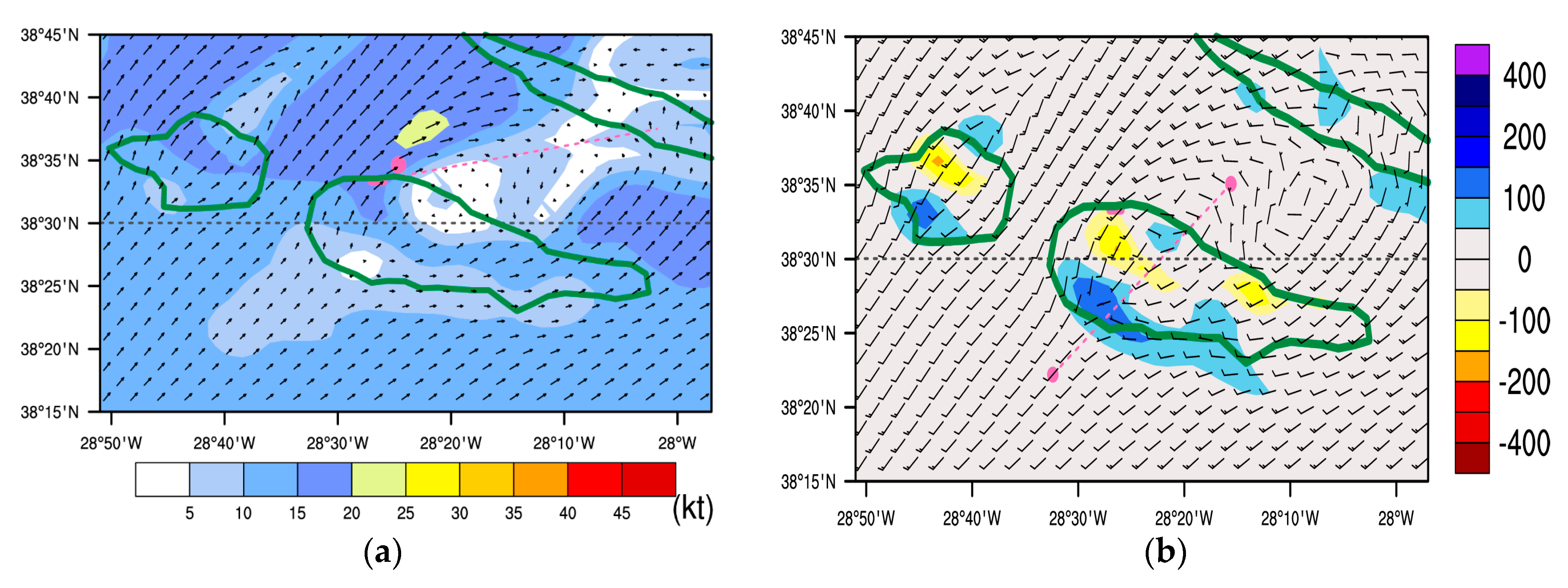
3.3.2. Characterization of Orographic Flow during Flight 2

The horizontal wind and vertical component of the absolute vorticity predicted by the AROME model at several heights are presented in Figure 11 for Flight 2. Figure 11a depicts a stagnation area in the windward direction of Pico Mountain and the occurrence of a flow splitting phenomenon in addition to a wake with reversed flow in the lee of the hill. This wake (at 40 m) consists of a pair of vortices, one with a clockwise rotation and negative absolute vorticity and another with a counter-clockwise rotation and positive vorticity. The wake structure exemplified in Figure 11a, which is visible below 600 m (not shown), resembles the results obtained by Smith and Grubišić [45] (p. 3747) in their study of Hawaii’s wake, which is described as comprising “two large, nearly steady vortices”. A similar structure with a pair of counter-rotating vortices downstream of the obstacle was also documented by Smolarkiewicz and Rotunno [7] (see their Figure 1c) and by Epifanio [4] (their Figure 3c). Moreover, the regime flow diagram of Figure A1b in Appendix A, which was used by Schär and Smith [39] and Grubišić et al. [5], accurately estimates this situation in which a wake displays reversed flow.
At higher levels, between 600 m and 850 m (Figure 11b,c), no lee vortices are present and the dipole of positive and negative vorticities is weaker and shifted to the east relative to lower levels, mainly at 850 m. At 1100 m, the incoming flow is mainly from the west and overcomes the mountain (Figure 11d). Finally, the analysis of Figure 11 suggests that the critical height in Flight 2 should be approximately 850 m, which is close to the estimate of the dividing streamline concept (see Table 3).
The horizontal wind speed at 40 m is depicted in Figure 12a, which shows that near the aircraft position, the wind speed varies between 15 and 20 kt (8–10 ms−1). It is also visible from this figure that the aircraft during the approach phase (pink dashed line in Figure 12a) has passed through the wake. Figure 12a and Figure 13 also show signs of a vertically propagating mountain wave, however, less energetic than the one seen on the day of Flight 1 (compared to Figure 10) and propagating to lower levels (up to 25000 ft or 7620 m), as is illustrated in Figure S6b. During Flight 2, the maximum vertical velocity on the leeward side of Pico Mountain (Figure 13b) is less than 150 ft/min (0.8 ms−1), while during Flight 1 the maximum vertical velocity was above 400 ft/min (2 ms−1). Upon propagation of this wave to the aerodrome (Figure 13a), it is seen that only a weak downdraft (less than 100 ft/min or 0.5 ms−1) lies atop it with no hints of updrafts along the flight path. In Figure 13b, the reversed flow associated with the lee vortices is also visible until about 2000 ft (610 m).

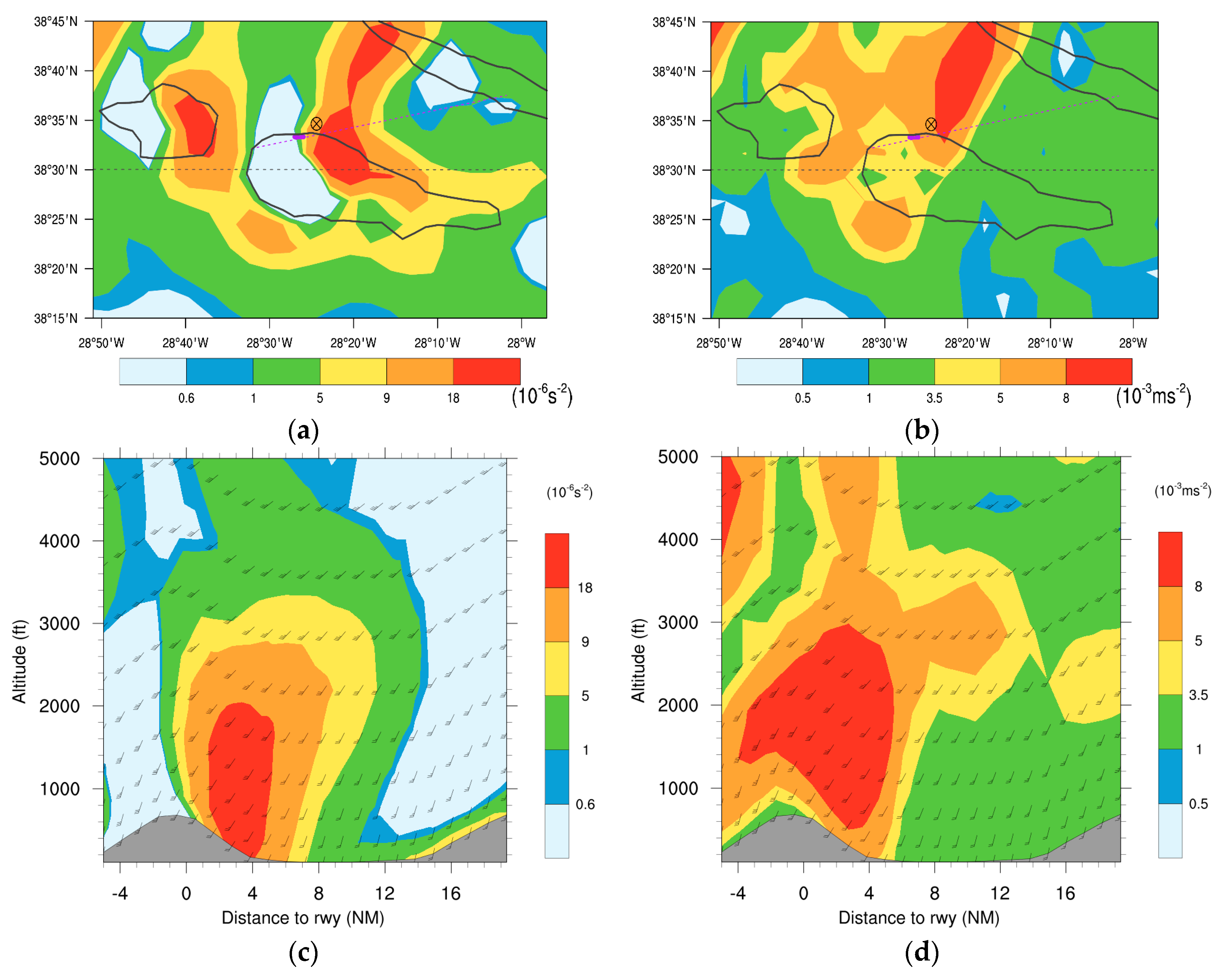
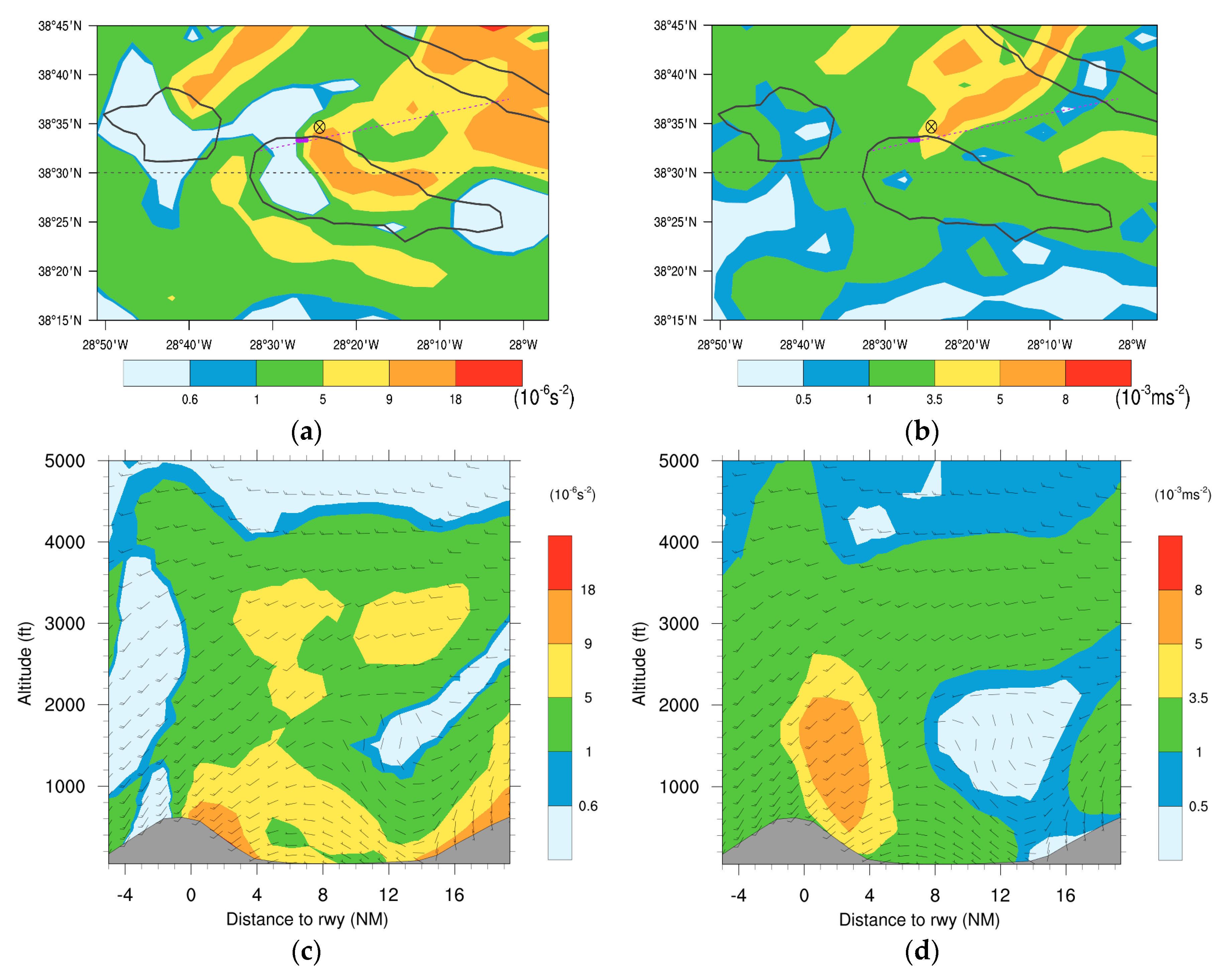
3.4. Turbulence Indicators

Turbulence indicators Ellrod TI2 and CAT1 at 66 m are presented in Figure 14a,b, for Flight 1. Both indicators show maximum values leeward of Pico mountain, with TI2 exceeding 18 × 10 6 s−2 and CAT1 exceeding 8 × 10 3 ms−2 in the proximity of the aerodrome where the incident occurred. The cross-section along the flight path shows that for a distance less than 5 NM (9.3 km) of the runway, between 300 and 1600 ft, TI2 and CAT1 reach values above 18 × 10 6 s−2 and 8 × 10 3 ms−2, respectively (Figure 14c,d). Comparing the indicators with the wind shear Intensity Factor “I” (Figure 15a,b), the aircraft experienced severe wind shear at these levels, suggesting that these values for TI2 and CAT1 could be tested as thresholds indicative of severe wind shear conditions. Ellrod TI1 (not shown in Figure 14) has a similar spatial pattern to TI2, but with lower values (Figure 15a). The Brown index is maximum over land near the LPPI aerodrome (not shown in Figure 14), exceeding 20 × 10−9 s−3 near the surface and decreasing drastically with height, reaching a value of 13 × 10−9 s−3 at 600 ft (Figure 15c).
The EDR indicator shows a different pattern when compared to others. EDR shows higher values over land than over sea, depicting a maximum value above 0.4 m2/3 s−1 near the top of Pico Mountain (Figure 16a). The higher values over land are consistent with higher roughness lengths (than over sea), which contribute to a higher mechanical production of turbulence [16]. At 66 m, EDR reaches a value between 0.35 and 0.4 m2/3 s−1 near the aerodrome (corresponding to moderate turbulence). Figure 16b shows that along the flight path, EDR decreases with height, varying from 0.35–0.4 m2/3 s−1 near the surface to 0.15–0.2 m2/3 s−1 at 2000 ft (610 m). It is interesting to mention that the thresholds applied in Figure 16 are lower than those presented in ICAO [43] but are those proposed recently [46], after a study by Sharman et al. [47] that showed that the thresholds in reference [43] were overestimated. According to reference [46], turbulence is severe when EDR ≥ 0.45 m2/3 s−1 and is moderate for EDR between 0.2 and 0.45 m2/3 s−1. Comparing EDR to the wind shear Intensity Factor “I” (Figure 15d), it is clear that in the presence of severe wind shear conditions, EDR has values between 0.2 and 0.25 m2/3 s−1 above 700 ft. For heights under 200 ft (61 m), EDR is close to 0.3, which suggests an underestimation of the severe wind shear conditions.
During Flight 2, the index Ellrod TI2 shows maximum values in the leeward region of the mountain and exhibits a value of 9 × 10 6 s−2 near the aircraft position (Figure 17a). The index CAT1 shows maximum values above 5 × 10 3 ms−2 downstream of Pico Aerodrome, close to the flight path (Figure 17b). Along the flight path itself, Ellrod TI2 reaches values above 9 × 10 6 s−2 below 500 ft (152 m), while CAT1 attains values between 4 × 10 3 ms−2 and 8 × 10 3 ms−2 below 900 ft or 274 m (Figure 17c,d and Figure S7), which are predominantly “moderate” wind shear conditions. The TI1 indicator is very similar to TI2 and the Brown index decreases again drastically with height, exhibiting values below 4 ×10⁻⁹ s−3 above 300 ft (Figure S7).
Analysis of EDR depicts the occurrence of “light” turbulence near the aerodrome for Flight 2 (Figure 18). The “I” factor is mostly consistent with this categorization as wind shear conditions reach intensities that are predominantly “light” for heights between 200–500 ft (61–152 m). Nevertheless, in some instants the wind shear was classified as “moderate”, while the EDR values above 400 ft are below 0.1 m2/3 s−1 suggesting the absence of turbulence or wind shear (Figure S7d).
This preliminary scrutiny of turbulence indicators suggests that CAT1, Ellrod TI2 and EDR could be applied together to arrive at a classification for the hazard level of turbulence. Moreover, preliminary thresholds for these indicators are proposed (Table A1), which should be subject to further validation, using more flight data.
As expected from their similarity in mathematical construction, both TKE and EDR evolve analogously during both flights (Figure S8a,b). In Flight 1, when the EDR indicator attains values of around 0.3 m2/3 s−1 (coinciding with “severe” wind shear conditions according to the “I” factor), TKE has values close to 4 m2s−2. During Flight 2, an EDR hovering near 0.1 m2/3 s−1 translated to a TKE value of about 0.5 m2s−2.
In order to certify that the turbulence was indeed predominantly greater for Flight 1 than for Flight 2, independently of the discrepant mean flow speeds in each case, the dimensionless turbulence intensity parameter ( T I = T K E / V h ), defined by Stull [16], was also plotted (Figure S9). It is clear from these results that the TI of Flight 1, with two maxima slightly above 0.25 (near 200 ft or 61 m and 1200 ft or 366 m), mostly exceeds that of Flight 2, with a maximum slightly above 0.15 (near 300 ft or 91 m).

3.5. Objective Verification of Wind Forecasts from AROME

The accuracy of AROME wind predictions is assessed by comparing them with data that was collected by SATA aircraft during Flights 1 and 2. Absolute errors of wind speed and direction are also mapped for each observation and forecast pair in Figure 19. The color coding for wind magnitude and its direction is based on ICAO guidelines [43] for operationally acceptable levels of forecast errors. For wind speed, an absolute value error of up to 5 kt (2.6 ms−1) was deemed operationally desirable. For the direction, this value is 20°. For Flight 1, there is a good agreement between observations and forecasts.
Values for the root mean square error (RMSE) and mean absolute error (MAE) regarding wind speed and direction are displayed in Table 4, showing that wind speed RMSE for Flight 1 is only slightly above operational recommendations (about 30% larger) and the RMSE for wind direction is 11.4°, well within the acceptable limits. The Flight 1 MAE for wind speed shows that the 2.6 ms−1 recommendation is exceeded by only 7% and the wind direction MAE is again within limits with a value of 8.1°.
During Flight 2, the RMSE and MAE for wind speed are 4.43 ms−1 and 3.77 ms−1 respectively, slightly over 30% larger than Flight 1 errors. For Flight 2 wind direction errors, the RMSE and MAE are around 83.3° and 65.4°. It is important to mention that when the wind speed is above 10 kt, the wind direction errors are inferior to 45° (see Figure S10). However, during Flight 2 at altitudes above 1200 ft, the wind is below 10 kt (Figure S4b) and at these levels, large errors (>120°) are found in the wind direction (Figure 4b, Figure S10). The limitations of NWP models in accurately forecasting the wind direction for weak winds was previously documented by Jiménez et al. [44], who showed that RMSE WDIR increases with decreasing wind speeds, reaching values over 70° for speeds under 2 kt (1 ms−1). It is also important to note that during Flight 2, a wake developed in the lee of Pico mountain in the vicinity of the flight path. In the wake region, the wind varies strongly over short distances (see Figure 12), implying that a small phase error may cause large errors in wind speed and/or wind direction. According to Ricard et al. [22], the effective resolution of the AROME model is about 9 times the grid spacing (i.e., 22 km), which may be insufficient to correctly resolve the wind variations within the lee wake.

4. Summary and Conclusions

The present article focuses on the orographic flow associated with Pico Mountain in the Azores in two different synoptic environments, using SATA airborne measurements and AROME forecasts. Aerial measurements were used to compute the wind shear intensity factor “I” according to Guan and Yong [25] and to categorize its severity according to four classes: “light”, “moderate”, “strong” and “severe”.
During the first scenario, a hard landing incident (Flight 1) occurred in Pico’s aerodrome. On this day, according to the AROME model, the upstream conditions were characterized by southwest winds with speeds of up to 40 kt (20 ms−1) in the ABL and stable stratification, which translated to a Froude number slightly above 1 near the mountain top. These conditions triggered the development of vertically propagating mountain waves, which created an undulation pattern of upward and downward motion downstream of Pico Mountain, leading to maximum vertical velocities above 400 ft/min (2 ms−1) and above 200 ft/min in the flight path. Based on ICAO Annex 3 guidelines [43], a mountain wave is deemed “severe” whenever downdrafts exceed 600 ft/min (3 ms−1) and “moderate” whenever they vary between 350 to 600 ft/min (1.75–3.0 ms−1). However, it is important to note that the AROME model may have underestimated the intensity of the vertical velocities, so this pattern of oscillating updraft/downdraft may have strongly contributed to the hard landing event. Furthermore, large wind speeds (38 kt or 20 ms−1) were registered close to 440 ft (107 m) and the wind shear intensity factor “I” based on airborne data showed that 36% of the approach phase (below 2100 ft or 640 m) occurred under “severe” wind shear conditions and 16% under “strong”. At the aerodrome, METAR observations showed southwest winds (18–21 kt or 9–11 ms−1) with gusts between 28 and 31 kt (14 and 16 ms−1).
During the second flight, the upstream conditions were characterized by southwest winds with speeds below 20 kt (10 ms−1) in the PBL and a temperature inversion in the layer between 860 to 1100 m. In this range, the Froude number is less than 0.5. According to previous studies, these conditions promote upstream stagnation and flow splitting with the formation of lee vortices in low levels with reversed flow, which was predicted by the AROME model. AROME forecasts for Flight 2 also showed a pattern of vertically propagating waves, but with smaller vertical velocities and shorter vertical propagation compared to Flight 1. According to airborne observations, Flight 2 occurred under wind shear conditions predominantly rated as “light” (68%) or “moderate” (29%), with its most intense class being “strong” (only during less than 4% of the landing phase).
Moreover, the pattern of several turbulence indicators derived from AROME forecasts was analyzed for both flights. All these indicators forecast higher values for Flight 1 than for Flight 2, which is consistent with the wind shear intensity factor “I” derived from airborne observations. As a result of the comparison between “I” and the AROME turbulence indicators, preliminary thresholds have been proposed for three indexes. In the future, however, more flights should be perused in order to verify the validity of such thresholds. The use of other wind shear and turbulence indicators derived from airborne data should also be tested.
Lastly, this study provides an objective verification of AROME wind forecasts, showing a good agreement with airborne observations for wind speeds above 10 kt, but a poor skill for weaker winds. For Flight 1, characterized by wind speeds over 30 kt (15 ms−1) during several instants, AROME forecasts show a good agreement with observations in terms of wind speed and direction, with an RMSE of 3.4 ms−1 and 11.4°, respectively. The MAE score is 2.8 ms−1 and 8.1° for wind speed and direction, respectively. During Flight 2, in the approach phase, the maximum wind speed is 22 kt (11 ms−1). In this case, AROME has an RMSE of 4.4 ms−1 and 83.3° for wind speed and wind direction. MAE revealed values of 3.8 ms−1 and 65.4° for the wind speed and direction. In particular, when the wind speed is below 10 kt (5 ms−1), large errors (>120°) in the wind direction can be found. This is a limitation of NWP models that was previously documented by Jiménez et al. [44] for the WRF model.
Strong ageostrophic winds often develop in coastal gaps or channels when an along-gap pressure gradient is created [48]. A gap flow may also contribute to reinforce the winds downstream of the strait between Faial and Pico islands. This hypothesis should be subject to future research.

Supplementary Materials

The following are available online at https://www.mdpi.com/2073-4433/10/7/350/s1, Figure S1: (a) Enlarged view of Pico Mountain and its Aerodrome (LPPI), (b) Location of Pico Aerodrome (LPPI) relative to Pico Mountain, Figure S2: Cross and headwind components, Figure S3: Boundaries for the classification of wind shear intensity, Figure S4: Wind profile along flight path according to aerial observations and AROME for (a) Flight 1, and (b) Flight 2, Figure S5: Absolute temperature and N profiles at point C for (a) Flight 1 and (b) Flight 2, Figure S6: (a) Vertically propagating mountain waves predicted by AROME during Flight 1, and (b) Flight 2, Figure S7: AROME turbulence indicators vs. the wind shear intensity factor I along the flight path during Flight 2. Figure S8: Variation of Turbulent Kinetic Energy (TKE) and Eddy Dissipation Rate (EDR) with Height for (a): Flight 1 and (b) Flight 2. Figure S9: Turbulence Intensity for both Flights. Figure S10: Absolute Value Wind Direction Errors versus Wind Speed for both Flights.

Author Contributions

Conceptualization, J.M., M.B.-P. and P.S.; software, J.M. and M.B.-P.; Analysis, J.M., M.B.-P. and P.S.; writing—original draft preparation, J.M. and M.B.-P.; writing—review and editing, J.M., M.B.-P. and P.S.; Figures, J.M. and M.B.-P.; supervision, M.B.-P. and P.S.

Funding

FCT - Portuguese Foundation for Science and Technology, under the project UID/AGR/04033/2019.

Acknowledgments

This work is supported by National Funds by FCT - Portuguese Foundation for Science and Technology, under the project UID/AGR/04033/2019. The authors are also thankful to SATA International – Azores Airlines, S.A. for providing the airborne data.

Conflicts of Interest

The authors declare no conflict of interest.

Appendix A

Figure A1. (a) Regime flow diagram adapted from Bauer et al. [2] for conditions of Flight 1; (b) Regime flow diagram adapted from Grubišić et al. [5] for conditions of Flight 2. Red mark indicates predicted states according to results from this study. Pico’s orography is approximately circular (unitary horizontal aspect ratio).
Atmosphere 10 00350 g0a1
Table A1. Suggested preliminary thresholds for three turbulence indicators. The thresholds values of EDR are only valid for heights below 500 ft (152 m).
Indicator“Strong”“Severe”
Ellrod TI2 [ 10 6 s 2 ] [ 9 , 16 [ [ 16 , + [
CAT1 [ 10 3 m s 2 ] [ 5 , 8 [ [ 8 , + [
EDR [ 0.3 , 0.35 [ [ 0.35 , + [

References

  1. Markowski, P.; Richardson, Y. Mesoscale Gravity Waves. In Mesoscale Meteorology in Midlatitudes, 1st ed.; Wiley-Blackwell: Hoboken, NJ, USA, 2010; pp. 161–180. [Google Scholar]
  2. Bauer, M.H.; Mayr, G.J.; Vergeiner, I.; Pichler, H. Strongly Nonlinear Flow over and around a Three-Dimensional Mountain as a Function of the Horizontal Aspect Ratio. J. Atmos. Sci. 2000, 57, 3971–3991. [Google Scholar] [CrossRef]
  3. Ólafsson, H.; Bougeault, P. Nonlinear Flow Past an Elliptic Mountain Ridge. J. Atmos. Sci. 1996, 53, 2465–2489. [Google Scholar] [CrossRef] [Green Version]
  4. Epifanio, C.C. Lee Vortices. In Encyclopedia of the Atmospheric Sciences; Cambridge University Press: Cambridge, UK, 2014; pp. 1150–1160. [Google Scholar]
  5. Grubišić, V.; Sachsperger, J.; Caldeira, R.M. Atmospheric Wake of Madeira: First Aerial Observations and Numerical Simulations. J. Atmos. Sci. 2015, 72, 4755–4776. [Google Scholar] [CrossRef] [Green Version]
  6. Heinze, R.; Raasch, S.; Etling, D. The Structure of Kármán Vortex Streets in the Atmospheric Boundary Layer derived from Large Eddy Simulation. Meteorol. Z. 2012, 21, 221–237. [Google Scholar] [CrossRef]
  7. Smolarkiewicz, P.K.; Rotunno, R. Low Froude-Number Flow Past Three-dimensional Obstacles. Part I: Baroclinically Generated Lee Vortices. J. Atmos. Sci. 1989, 46, 1154–1164. [Google Scholar] [CrossRef]
  8. Li, L.; Chen, Y.-L. Numerical Simulations of Two Trapped Mountain Lee Waves Downstream of Oahu. J. Appl. Meteorol. Climatol. 2017, 56, 1305–1324. [Google Scholar] [CrossRef]
  9. Keller, T.L.; Trier, S.B.; Hall, W.D.; Sharman, R.D.; Xu, M.; Liu, Y. Lee Waves Associated with a Commercial Jetliner Accident at Denver International Airport. J. Appl. Meteorol. Climatol. 2015, 54, 1373–1392. [Google Scholar] [CrossRef] [Green Version]
  10. Parker, T.J.; Lane, T.P. Trapped Mountain Waves during a Light Aircraft Accident. Aust. Meteorol. Oceanogr. J. 2013, 63, 377–389. [Google Scholar] [CrossRef]
  11. Caldeira, R.M.A.; Tomé, R. Wake Response to an Ocean-Feedback Mechanism: Madeira Island Case Study. Bound. Layer Meteorol. 2013, 148, 419–436. [Google Scholar] [CrossRef] [Green Version]
  12. Couvelard, X.; Caldeira, R.M.A.; Araújo, I.B.; Tomé, R. Wind Meditated Vorticity-generation and Eddy-confinement, Leeward of the Madeira Island: 2008 Numerical Case Study. Dyn. Atmos. Oceans 2012, 58, 128–149. [Google Scholar] [CrossRef]
  13. Barata, J.M.M.; Medeiros, R.C.; Silva, A.R.R. An Experimental Study of Terrain-Induced Airflow at the LPPI Airport. In Proceedings of the 10th AIAA Aviation Technology, Integration, and Operations (ATIO) Conference, Fort Worth, TX, USA, 13–15 September 2010; American Institute of Aeronautics and Astronautics: Reston, VA, USA, 2010; pp. 1–8. [Google Scholar]
  14. Sayers, D.; Stewart, M. Background Information. In Azores, 6th ed.; The Globe Pequot Press Inc.: Guilford, CT, USA, 2016; pp. 2–3. [Google Scholar]
  15. Sharman, R.D.; Pearson, J.M. Prediction of Energy Dissipation Rates for Aviation Turbulence. Part I: Forecasting Nonconvective Turbulence. J. Appl. Meteor. Climatol. 2017, 56, 317–337. [Google Scholar] [CrossRef]
  16. Stull, R.B. An Introduction to Boundary Layer Meteorology; Springer: Berlin, Germany, 1988; 666p. [Google Scholar]
  17. Jiménez, P.A.; Dudhia, J. Improving the Representation of Resolved and Unresolved Topographic Effects on Surface Wind in the WRF Model. J. Appl. Meteorol. Climatol. 2012, 51, 300–316. [Google Scholar] [CrossRef] [Green Version]
  18. Chow, F.K.; Street, R.L. Evaluation of Turbulence Closure Models for Large-Eddy Simulation over Complex Terrain: Flow over Askervein Hill. J. Appl. Meteorol. Climatol. 2009, 48, 1050–1065. [Google Scholar] [CrossRef]
  19. Svensson, G.; Holtslag, A.A.M. Analysis of Model Results for the Turning of the Wind and Related Momentum Fluxes in the Stable Boundary Layer. Bound. Layer Meteorol. 2009, 132, 261–277. [Google Scholar] [CrossRef]
  20. Brown, A.R.; Beljaars, A.C.M.; Hersbach, H.; Hollingsworth, A.; Miller, M.; Vasiljevic, D. Wind turning across the marine atmospheric boundary layer. Q. J. R. Meteorol. Soc. 2005, 131, 1233–1250. [Google Scholar] [CrossRef]
  21. Brown, A.R.; Beare, R.J.; Edwards, J.M.; Lock, A.P.; Keogh, S.J.; Milton, S.F.; Walters, D.N. Upgrades to the boundary-layer scheme in the Met Office numerical weather prediction model. Bound. Layer Meteor. 2008, 128, 117–132. [Google Scholar] [CrossRef]
  22. Ricard, D.; Lac, C.; Riette, S.; Legrand, R.; Mary, A. Kinetic energy spectra characteristics of two convection-permitting limited-area models AROME and Meso-NH. Q. J. R. Meteorol. Soc. 2013, 139, 1327–1341. [Google Scholar] [CrossRef]
  23. Woodfield, A.A.; Woods, J.F. Worldwide experience of windshear during 1981–1982. In AGARD Flight Mechanics Panel Conf. on Flight Mechanics and System Design Lessons from Operational Experience; AGARD CP; NATO-STO: Brussel, Belgium, 1983; Volume 347, 28p. [Google Scholar]
  24. International Civil Aviation Organization (ICAO). Manual on Low-level Wind Shear, 1st ed.; International Civil Aviation Organization: Montreal, QC, Canada, 2005; p. 213. [Google Scholar]
  25. Guan, W.-L.; Yong, K. Review of Aviation Accidents Caused by Wind Shear and Identification Methods. J. Chin. Soc. Mech. Eng. 2002, 23, 99–110. [Google Scholar]
  26. Seity, Y.; Brousseau, P.; Malardel, S.; Hello, G.; Bénard, P.; Bouttier, F.; Lac, C.; Masson, V. The AROME-France Convective-Scale Operational Model. Mon. Weather Rev. 2011, 139, 976–991. [Google Scholar] [CrossRef] [Green Version]
  27. Cuxart, J.; Bougeault, P.; Redelsperger, J.-L. A Turbulence Scheme Allowing for Mesoscale and Large-eddy Simulations. Q. J. R. Meteorol. Soc. 2006, 126, 1–30. [Google Scholar] [CrossRef]
  28. Sutherland, B.R. Generation Mechanisms. In Internal Gravity Waves; Cambridge University Press: Cambridge, UK, 2018; pp. 284–285. [Google Scholar]
  29. Lynch, A.H.; Cassano, J.J. Mountain Weather. In Atmospheric Dynamics; Wiley: Hoboken, NJ, USA, 2006; pp. 209–232. [Google Scholar]
  30. Holton, J. An Introduction to Dynamic Meteorology, 4th ed.; Elsevier Inc.: Amsterdam, The Netherlands, 2004; Volume 88, 535p. [Google Scholar]
  31. Sheridan, P.F.; Vosper, S.B. A Flow Regime Diagram for Forecasting Lee Waves, Rotors and Downslope Winds. Meteorol. Appl. 2006, 13, 179–195. [Google Scholar] [CrossRef]
  32. Sheppard, P.A. Airflow over Mountains. Q. J. R. Meteorol. Soc. 1956, 82, 528–529. [Google Scholar] [CrossRef]
  33. Sha, W.; Nakabayashi, K.; Ueda, H. Numerical Study on Flow Pass of a Three-dimensional Obstacle under a Strong Stratification Condition. J. Appl. Meteorol. 1998, 37, 1047–1054. [Google Scholar] [CrossRef]
  34. Vosper, S.B.; Gardner, B.A. Measurements of the Near Surface Flow over a Hill. Q. J. R. Meteorol. Soc. 2002, 128, 2257–2280. [Google Scholar] [CrossRef]
  35. Jiang, Q.; Doyle, J.D.; Smith, R.B. Blocking, Descent and Gravity Waves: Observations and Modelling of a MAP Northerly Föhn Event. Q. J. R. Meteorol. Soc. 2005, 131, 675–701. [Google Scholar] [CrossRef]
  36. Trombetti, F.; Tampieri, F. An Application of the Dividing-Streamline Concept to the Stable Airflow over Mesoscale Mountains. Mon. Weather Rev. 1987, 115, 1802–1806. [Google Scholar] [CrossRef] [Green Version]
  37. Wooldridge, G.L.; Fox, D.G.; Furman, R.W. Air-Flow Patterns over and around a Large 3-Dimensional Hill. Meteorol. Atmos. Phys. 1987, 37, 259–270. [Google Scholar] [CrossRef]
  38. Vosper, S.B. Inversion Effects on Mountain Lee Waves. Q. J. R. Meteorol. Soc. 2004, 130, 1723–1748. [Google Scholar] [CrossRef]
  39. Schär, C.; Smith, R.B. Shallow-Water Flow past Isolated Topography. Part I: Vorticity Production and Wake Formation. J. Atmos. Sci. 1993, 50, 1373–1400. [Google Scholar] [Green Version]
  40. Gill, P.G.; Buchanan, P. An Ensemble based Turbulence Forecasting System. Meteorol. Appl. 2014, 21, 12–19. [Google Scholar] [CrossRef]
  41. Sharman, R.; Tebaldi, C.; Wiener, G.; Wolff, J. An Integrated Approach to Mid- and Upper-Level Turbulence Forecasting. Weather Forecast. 2006, 21, 268–287. [Google Scholar] [CrossRef]
  42. Frech, M.; Holzäpfel, F.; Tafferner, A.; Gerz, T. High-Resolution Weather Database for the Terminal Area of Frankfurt Airport. Am. Meteorol. Soc. 2007, 46, 1913–1932. [Google Scholar] [CrossRef] [Green Version]
  43. International Civil Aviation Organization (ICAO). Meteorological Service for International Air Navigation: Annex 3 to the Convention on International Civil Aviation, 20th ed.; International Standards and Recommended Practices Technical Report; International Civil Aviation Organization: Montreal, QC, Canada, 2007; p. 218. [Google Scholar]
  44. Jiménez, P.A.; Dudhia, J. On the Ability of the WRF Model to Reproduce the Surface Wind Direction over Complex Terrain. J. Appl. Meteorol. Climatol. 2013, 52, 1610–1617. [Google Scholar] [CrossRef]
  45. Smith, R.B.; Grubišić, V. Aerial Observations of Hawaii’s Wake. J. Atmos. Sci. 1993, 50, 3728–3750. [Google Scholar] [CrossRef]
  46. International Civil Aviation Organization (ICAO). Meeting of the Meteorology Panel (METP): Proposed Revision to Eddy Dissipation Rate (EDR) Values in Annex 3; International Civil Aviation Organization: Montreal, QC, Canada, 2018; pp. 1–6. [Google Scholar]
  47. Sharman, R.D.; Cornman, L.B.; Meymaris, G.; Pearson, J.; Farrar, T. Descriptions and Derived Climatologies of Automated in Situ Eddy-Dissipation-Rate Reports of Atmospheric Turbulence. J. Appl. Meteorol. Climatol. 2014, 53, 1416–1432. [Google Scholar] [CrossRef]
  48. Colle, B.A.; Mass, C.F. High-Resolution Observations and Numerical Simulations of Easterly Gap Flow through the Strait of Juan de Fuca on 9–10 December 1995. Mon. Weather Rev. 2000, 128, 2398–2422. [Google Scholar] [CrossRef]
Figure 1. Macroscopic view of Pico Island’s location relative to Mainland Portugal.
Atmosphere 10 00350 g001
Figure 2. Approximate flight path (blue dashed line) and AROME orography. Shading shows elevation in meters. Pink marker shows the aerodrome location. “AB” and “CD” are endpoints of cross-sections analyzed in subsequent sections.
Atmosphere 10 00350 g002
Figure 3. Theoretical illustration of the flow splitting phenomenon with green arrows depicting airflow. Potential temperature profile is shown in blue. The critical and inversion heights, h c and z i respectively, are also illustrated.
Atmosphere 10 00350 g003
Figure 4. Variation of wind speed with altitude along the flight path, below 5000 ft (1524 m), for: (a) Flight 1; (b) Flight 2.
Atmosphere 10 00350 g004
Figure 5. Relative frequency per wind shear intensity category for: (a) Flight 1; and (b) Flight 2.
Atmosphere 10 00350 g005
Figure 6. Mean sea level pressure (in hPa) and 10 m wind (kt) based on ECMWF analysis for: (a) Flight 1; (b) Flight 2.
Atmosphere 10 00350 g006
Figure 7. Vertical profile of Froude number (from AROME forecasts) for both flights.
Atmosphere 10 00350 g007
Figure 8. AROME absolute vorticity and wind vectors for Flight 1 at an altitude of: (a) 30 m; (b) 500 m. Dark arrows represent wind vectors.
Atmosphere 10 00350 g008
Figure 9. (a) Horizontal wind at 680 ft (207 m) for Flight 1; (b) Maximum vertical velocity under 6000 ft (1829 m) for Flight 1. Both fields are from AROME forecasts. Shading in (a) represents the wind speed in kt and the pink dot identifies the approximate aircraft position at this level. Pink dashed line identifies the approximate aircraft trajectory. Shading in (b) represents intensity in ft/min, positive values indicate upward vertical velocity and negative values represent downward vertical velocity. The pink dots are the points C and D shown in Figure 2, which are the endpoints of the cross-section (dashed pink line) used in the next figures.
Atmosphere 10 00350 g009
Figure 10. Vertical cross-section of the vertical velocity of AROME through (a) line A–B on Figure 2 and (b) line C–D on Figure 2, for Flight 1. Shading represents intensity in ft/min, positive values indicate upward vertical velocity and negative values represent downward vertical velocity. The altitude scale of (a) is half of the corresponding scale of (b).
Atmosphere 10 00350 g010
Figure 11. AROME absolute vorticity and wind vectors for Flight 2 at an altitude of: (a) 40 m; (b) 640 m; (c) 850 m; (d) 1100 m. Dark arrows represent wind vectors.
Atmosphere 10 00350 g011
Figure 12. (a) Horizontal wind at 135 ft (40 m) for Flight 2.; (b) Maximum vertical velocity component under 6000 ft (1829 m) for Flight 2. Both fields are from AROME forecasts. Shading in (a) represents the wind speed in kt and the pink dot identifies the approximate aircraft position at this level. Pink dashed line identifies the approximate aircraft trajectory. Shading in (b) represents intensity in ft/min, positive values indicate upward vertical velocity and negative values represent downward vertical velocity. The pink dots are the points C and D shown in Figure 2, which are the endpoints of cross-section (dashed pink line) used in the next figures.
Atmosphere 10 00350 g012
Figure 13. Vertical cross-section of the vertical velocity of AROME through (a) line A-B in Figure 2 and (b) line C–D in Figure 2, for Flight 2. Shading represents intensity in ft/min, positive values indicate upward vertical velocity and negative values represent downward vertical velocity. The altitude scale of (a) is half of the corresponding scale of (b).
Atmosphere 10 00350 g013
Figure 14. Horizontal variation of (a) Ellrod TI2 and (b) CAT1 at 66 m for Flight 1. Dotted pink line shows aircraft trajectory and pink bar locates the aerodrome. The circled “x” mark identifies the approximate aircraft position at 66 m. Cross-sectional variation of (c) Ellrod TI2 and (d) CAT1.
Atmosphere 10 00350 g014
Figure 15. AROME turbulence indicators (bottom x-axis) vs. the wind shear intensity factor “I” (top x-axis), along the flight path during Flight 1. Ellrod TI1, TI2 and Brown indicators are shown in (a) and (c), respectively. Solid red lines in (b) and (d) indicate CAT1 and EDR values, respectively.
Atmosphere 10 00350 g015
Figure 16. (a) Horizontal representation of EDR during Flight 1. The circled “X” mark identifies aircraft position at 66 m. (b) Cross-sectional representation of EDR.
Atmosphere 10 00350 g016
Figure 17. Horizontal variation of (a) Ellrod TI2 and (b) CAT1 at 66 m for Flight 2. Dotted pink line shows the aircraft trajectory and pink bar indicates the aerodrome. The circled “X” mark identifies the approximate aircraft position at 66 m. Cross-sectional variation of (c) Ellrod TI2 and (d) CAT1.
Atmosphere 10 00350 g017
Figure 18. (a) Horizontal representation of EDR during Flight 2. The circled “X” mark identifies approximate aircraft position at 66 m. (b) Cross-sectional representation of EDR.
Atmosphere 10 00350 g018
Figure 19. Absolute value differences for wind speed and direction for: (a) Flight 1 and (b) Flight 2.
Atmosphere 10 00350 g019
Table 1. Wind data (velocity in knots) based on METAR (Meteorological Aerodrome Reports) at Pico aerodrome at the time of flights. The crosswind ( W C H ) is from the left if negative. Negative values of W H D indicate headwinds. T1 and T2 are approximate landing times for Flights 1 and 2.
FlightTimeWind DirectionWind SpeedGust W H D W C H G W H D G W C H
Flight 1T1220°1828−12−14−18−21
T1+1hr220°2131−13−16−20−24
Flight 2T2200°13−4−12
T2+0.5hr210°12−6−10
Table 2. Classification of wind shear intensity for three lowest altitudes in Flights 1 and 2.
FlightAltitude d V d t ( m s 2 ) V V ClassificationRating
Flight 1228 ft (69 m)1.6490.170Severe4
164 ft (50 m)8.8200.476Severe4
90 ft (27 m)2.9620.138Severe4
Flight 2214 ft (65 m)0.2650.015Light1
169 ft (52 m)0.2640.015Light1
128 ft (39 m)0.7290.042Moderate2
Table 3. Froude number and related results by flight for Point C in Figure 2 with h c 1 , h c 2 , z i in meters.
ParameterFlight 1Flight 2
F r (Equation (3))0.950.42
F r h (Equation (6))0.900.31
F r i (Equation (7)) 0.92
h c 1 (Equation (5))107855
h c 2 (Equations (3),(6))60696
z i 872
Table 4. Summary of RMSE and MAE for wind speed and direction for both flights.
FlightRMSEWSPD [ms−1]RMSEWDIR [deg]MAEWSPD [ms−1]MAEWDIR [deg]
Flight 13.411.42.88.1
Flight 24.483.33.865.4

