Article

Lessons from Inter-Comparison of Decadal Climate Simulations and Observations for the Midwest U.S. and Great Lakes Region

by
Ashish Sharma
1,2,*,
Alan F. Hamlet
3 and
Harindra J.S. Fernando
3
1
Climate and Atmospheric Science Section, Illinois State Water Survey, Prairie Research Institute, University of Illinois at Urbana-Champaign, 2204 Griffith Dr., Champaign, IL 61820, USA
2
Department of Atmospheric Sciences, University of Illinois at Urbana-Champaign, 1301 W Green St., Urbana, IL 61801, USA
3
Department of Civil & Environmental Engineering and Earth Sciences (CEEES), University of Notre Dame, 156 Fitzpatrick Hall, Notre Dame, IN 46556, USA
*
Author to whom correspondence should be addressed.
Atmosphere 2019, 10(5), 266; https://doi.org/10.3390/atmos10050266
Submission received: 21 April 2019 / Revised: 8 May 2019 / Accepted: 11 May 2019 / Published: 13 May 2019
(This article belongs to the Special Issue Regional Climate Modeling: Ocean–Atmosphere Coupling)

Abstract

:
Even with advances in climate modeling, meteorological impact assessment remains elusive, and decision-makers are forced to operate with potentially malinformed predictions. In this article, we investigate the dependence of the Weather Research and Forecasting (WRF) model simulated precipitation and temperature at 12- and 4-km horizontal resolutions and compare it with 32-km NARR data and 1/16th-degree gridded observations for the Midwest U.S. and Great Lakes region from 1991 to 2000. We used daily climatology, inter-annual variability, percentile, and dry days as metrics for inter-comparison for precipitation. We also calculated the summer and winter daily seasonal minimum, maximum, and average temperature to delineate the temperature trends. Results showed that NARR data is a useful precipitation product for mean warm season and summer climatological studies, but performs extremely poorly for winter and cold seasons for this region. WRF model simulations at 12- and 4-km horizontal resolutions were able to capture the lake-effect precipitation successfully when driven by observed lake surface temperatures. Simulations at 4-km showed negative bias in capturing precipitation without convective parameterization but captured the number of dry days and 99th percentile precipitation extremes well. Overall, our study cautions against hastily pushing for increasingly higher resolution in climate studies, and highlights the need for the careful selection of large-scale boundary forcing data.

1. Introduction

The Midwest United States (U.S.) and the Great Lakes region are one of the world’s most productive agricultural landscapes with the world’s largest freshwater ecosystems and several large urban centers. The regional climate of the region is influenced by large-scale atmospheric circulations (e.g., moisture from the Gulf of Mexico in the south and arctic air outbreaks from the north), convective activity, and ice cover/water temperature in the Great Lakes (e.g., [1]). This region is usually fertile and has been extensively drained for agriculture. These factors contribute to large seasonal and daily variations in air temperature, including hot summers, cold winters, and occasional periods of drought and deluge. In recent decades, a statistically significant warming trend has been observed over the region [2,3,4,5]. The region exhibits warming with increasing latitudes.
The Midwest U.S. also has experienced two record-breaking floods in the last 20 years [6], strong heat waves have been more frequent [7], and extreme precipitation frequency has doubled relative to the last century [8]. Based on a special report for the Environmental Law and Policy Center and the Chicago Council on Global Affairs, there is a generally positive trend in annual precipitation for U.S. states bordering the Great Lakes for present-day (1986–2016) relative to 1901–1960, but with strong local variations in the trend across the states (http://elpc.org/glclimatechange/). There is an approximate 10% increase in annual precipitation averaged over the Great Lakes states [9]. The region has also recently witnessed unprecedented extreme changes in the timing of precipitation and runoff, with important implications for flooding, soil erosion, nutrient export, and agricultural practices [10,11]. Warm, wet winters are producing extensive early-season flooding, which threatens people and infrastructure [12]. In addition, an increase in population and associated infrastructure have made the region more vulnerable to flooding, irrespective of how humans are altering the climate itself. For example, the extreme storms experienced by the Great Lakes cities in the last 30 years or so have far exceeded the current design standards for infrastructure and have caused extensive damage. Damages in and around Calgary, Alberta exceeded $1.7B (CA $), and Toronto sustained more than $900M (CA $). In February 2018, the St. Joseph River near South Bend experienced a 2500-year flood, due to an intense atmospheric river and rain-on-snow event.
Future climate change projections for the Midwest region suggest increasing temperature and weather extremes, with regional warming up to 10 °C by 2100 [13]. Thus, the changes in temperature and precipitation, as well as future changes in the extremes of the distribution of temperature and precipitation, pose challenges for energy production, ecological conservation, human health, water resource management, and agricultural productivity of this region (IPCC [14,15]).
These adverse changes create challenges for water resource management [16,17], sustainable and resilient design of infrastructure [18], design of urban systems [19,20,21,22,23,24,25,26], ecosystem management [27,28,29,30], and regional impacts on agricultural land management and production [31]. These diverse climate change impact pathways highlight the need to evaluate the most commonly available observational and simulated datasets to determine the effectiveness of climate models in realistically capturing observed climate trends, variability, and extremes that contribute to impacts.
Generally, observational meteorological datasets are sparse and consist of near-surface observations of precipitation and temperature. The measurement of other variables, such as humidity and solar radiation, is relatively rare, and direct observations are, in isolation, often insufficient to characterize conditions with useful spatial coverage. Likewise, experimental field data (e.g., from radiosondes) are available in a few locations, but these kinds of observations are very limited. Therefore, climate models have proven to be a complementary tool to fill in the data gaps in space and time. Nonetheless, the realistic simulation of rainfall and temperature variation, especially at local scales, in climate models remains a significant challenge. For example, the current global climate models (GCMs) lack the capability of representing the multiscale cloud and precipitation [32]. RCMs have more realistic rainfall than global climate models [33,34,35], providing future projections with greater confidence. Thus, regional simulations constrained with large-scale forcing are crucial for determining local climate extremes, and hence they are imperative for climate change planning for impact pathways related to human and natural systems [36,37]. Dynamical and statistical downscaling methods provide finer spatial resolution information for long-and short-term climate impact assessments. However, the dynamically downscaled regional climate simulations have shown a higher skill in capturing atmospheric variability [38,39,40,41]. Furthermore, literature shows that data assimilation (nudging), especially the spectral nudging technique within the dynamical downscaling framework, adds more variability and improves the model’s skill at smaller scales [42,43].
Interestingly, limited effort has been invested in validating the input large-scale forcing datasets for regional climate models, especially in the context of extremes. This oversight may lead to the inadequate understanding of biases in model outputs. At the same time, there is a debate in the research community on the importance of increasing the spatial resolution of RCMs in simulating climate. Thus, the overall goal of this article is to evaluate multiple RCM model outputs at different resolutions (12- and 4-km) and NARR datasets at 32-km resolution (a high-resolution NCEP model dataset with assimilated observations) with commonly available gridded station observational data. Note, henceforth ‘horizontal grid increments’ from the RCM will be called ‘resolution’ in the paper [44,45,46,47].

2. Methods

2.1. Gridded Observations

We used a gridded observational meteorological dataset at daily timescales and 1/16th-degree (approx. 5 km) resolution over the Midwest and Great Lakes region. This dataset used a hybrid product based on interpolated station records from the Daily Global Historical Climatology Network (GHCN-Daily) station records, bias adjusted station records in Canada and regridded National Center for Atmospheric Research (NCAR) Reanalysis [48] wind speed data. Gridded temperature and precipitation products are based on techniques first developed by Maurer et al. [49] and Hamlet and Lettenmaier [50]. Irregularly spaced meteorological observation station records were regridded using the SyMAP (Synteny Mapping and Analysis Program) algorithm [51], which is an inverse distance squared weighting scheme. The scheme also considered the relative position of stations that are potentially cross-correlated with each other. In addition, adjustments for precipitation gauge undercatch in the U.S. data were applied to the gridded precipitation products based on empirical estimates of the catch ratio (CR) (defined as the ratio of long-term measurements of precipitation from a standard 8-in U.S. precipitation gauge to those from an accurate reference precipitation gauge) [52]. The estimate of CR varies as a function of precipitation type (snow, mixed rain, and rain) and wind speed [53]. Having established the CR for the meteorological conditions in each day, daily precipitation values were then adjusted by multiplying by 1/CR. Precipitation undercatch in Canada was corrected by interpolating daily station records with undercatch corrections already applied in previous efforts [54]. Additional details of this gridded meteorological dataset are presented in Byun and Hamlet [13].

2.2. NARR Datasets

We used time-varying, large-scale, 3-h National Centers for Environmental Prediction (NCEP) North American Regional Reanalysis (NARR) simulations at 32-km resolution (http://rda.ucar.edu/datasets/ds608.0/) as one of the datasets for comparison. NARR is a common dataset used by planners to make impact decisions in the United States and Canada. The research community uses NARR for creating climate and hydrology products. NARR model output is often downscaled to higher resolutions (e.g., 1–4 km) for assessing local climate vulnerabilities. The quality of NARR data has been evaluated with surface stations and sounding measurements [55]. Hence, it has been used in numerous studies for the validation of regional climate simulations in North America (e.g., [56]).

2.3. WRF Model Implementation

This study used the Weather Research and Forecasting model (WRF model, Version 3.6.1) [57]. This is a non-hydrostatic, compressible model used extensively at multiple resolutions ranging from meso-gamma (2–20 km) to local scales (~50 m) [22,24,58,59,60,61,62,63]. For the experiments in this study, the model was configured such that the outer domain covering most of North America at 12-km resolution (600 × 516 grid points) is centered at 52.24°N and 105.5°W. The inner domain at 4-km resolution (420 × 366 grid points) covers the Great Lakes megaregion. Note, the outer 12-km domain is big enough to account for all large-scale processes impacting the inner 4-km domain of our interest. Note, we settled for the innermost domain’s resolution to be 4-km and not higher than that, as a tradeoff between computational requirements for our large-scale and long-term climate simulations. The model had 50 pressure-based terrain-following vertical levels from the surface to 100 hPa. High-resolution static fields were used to the corresponding nested domains. The two-way nested model domains with terrain height are shown in Figure 1a. Figure 1b shows eight U.S. states surrounding the Great Lakes region (viz., Illinois, Indiana, Michigan, Minnesota, New York, Ohio, Pennsylvania and Wisconsin) along with the Canadian province Ontario in the north of the Great Lakes (Figure 1b).
Time-varying, large-scale, 6-hourly National Center for Environmental Prediction (NCEP)-U.S. Department of Energy (DOE) Atmospheric Model Intercomparison Project II reanalysis datasets (NCEP-R2) [64] at T62 Gaussian grids and 17 pressure levels were applied as lateral boundary conditions. Instantaneous model outputs at 3-hour intervals were used for analysis. Since the Great Lakes themselves have a strong influence on the regional and local climate, sea surface temperature (SST) and lake surface temperature (LST) were updated at the same interval as large-scale NCEP-R2 boundary conditions. This helped to provide a more accurate lower-boundary condition and capture the possible lake effects in the WRF model. In addition, we employed spectral nudging for horizontal winds, temperature, and geopotential height at the outer domain for the whole time-period to retain the representation of large-scale dynamics. Note, the variables in the planetary boundary layer (PBL), such as pressure and moisture, were not nudged because there is a strong coupling of the atmosphere and land surface, and we allowed the atmospheric state at lower levels to adjust freely to surface properties and forcings. For a better representation of landuse, we used 30-m 2006 National Land Cover Data set (NLCD 2006) [65] regridded for both respective domain resolutions.
WRF model has multiple parameterizations for microphysics, convection, radiation, boundary layer, and surface. Based on anteceded research over the region [20,24,43], we utilized the WRF Single-Moment six-class graupel scheme (WSM6) [66] for microphysics for its robustness in accounting for different heat and moisture tendencies in the atmosphere. We incorporated the Dudhia scheme [67] for shortwave and the Rapid Radiative Transfer Model (RRTM) for longwave radiation parameterizations [68]. The Monin–Obukhov similarity scheme based on Carlson–Boland viscous sub-layer and standard similarity functions from look-up tables was used for the surface layer, and the Yonsei University scheme [69] for PBL, and a four-layer Noah land surface model (LSM) [70] for surface physics. Subgrid-scale cumulus convective parameterization was turned on only for the outer domain (12-km) invoking the Kain–Fritsch scheme [71]. Since many cumulus parameterizations are poorly posed at 4-km grid spacing, the rationale behind the choice of the Kain–Fritsch scheme was that it activates for most of the cumulus events and yields more realistic precipitation features than fully explicit simulations for the Great Lakes region [72,73,74] and other regions (e.g., [59,75]).

2.4. Experimental Design

We performed WRF simulations for a period of 10 years from 1991 to 2000. The model was reinitialized for large-scale forcings (both atmospheric and surface) every year as previous studies have shown that reinitializations for long-term climate improve not only the forcing variables (e.g., pressure, temperature, wind, and moisture) but also the model diagnostic variables (e.g., precipitation) [56,76,77,78,79,80,81]. A 24-h spin up time was used for each year. For the experiment, publicly available NARR datasets were cropped and resized to domain d02. Note, the gridded observations over inner domain cover only the neighboring Great Lakes states and not the rectangular domain d02.
In the analysis, we used precipitation and temperature variables in our assessment. For all datasets, daily mean, maximum, and minimum values were calculated. We used decadal averages of daily climatology (based on daily means) and interannual variability (based on the standard deviations of daily means), percentile and dry days as metrics for inter-comparison for precipitation. We also calculated decadal averages of summer and winter seasonal minimum, maximum, and average daily temperature to delineate the temperature trends. Note, gridded observations lack data for some of the regions in domain 2. For statistical analysis, we did not account for those regions in the simulated datasets where observations were missing. Furthermore, note that gridded observations are missing over the Great Lakes themselves, due to insufficient meteorological stations over open water to support a gridded product.

3. Results

3.1. Gridded Observations

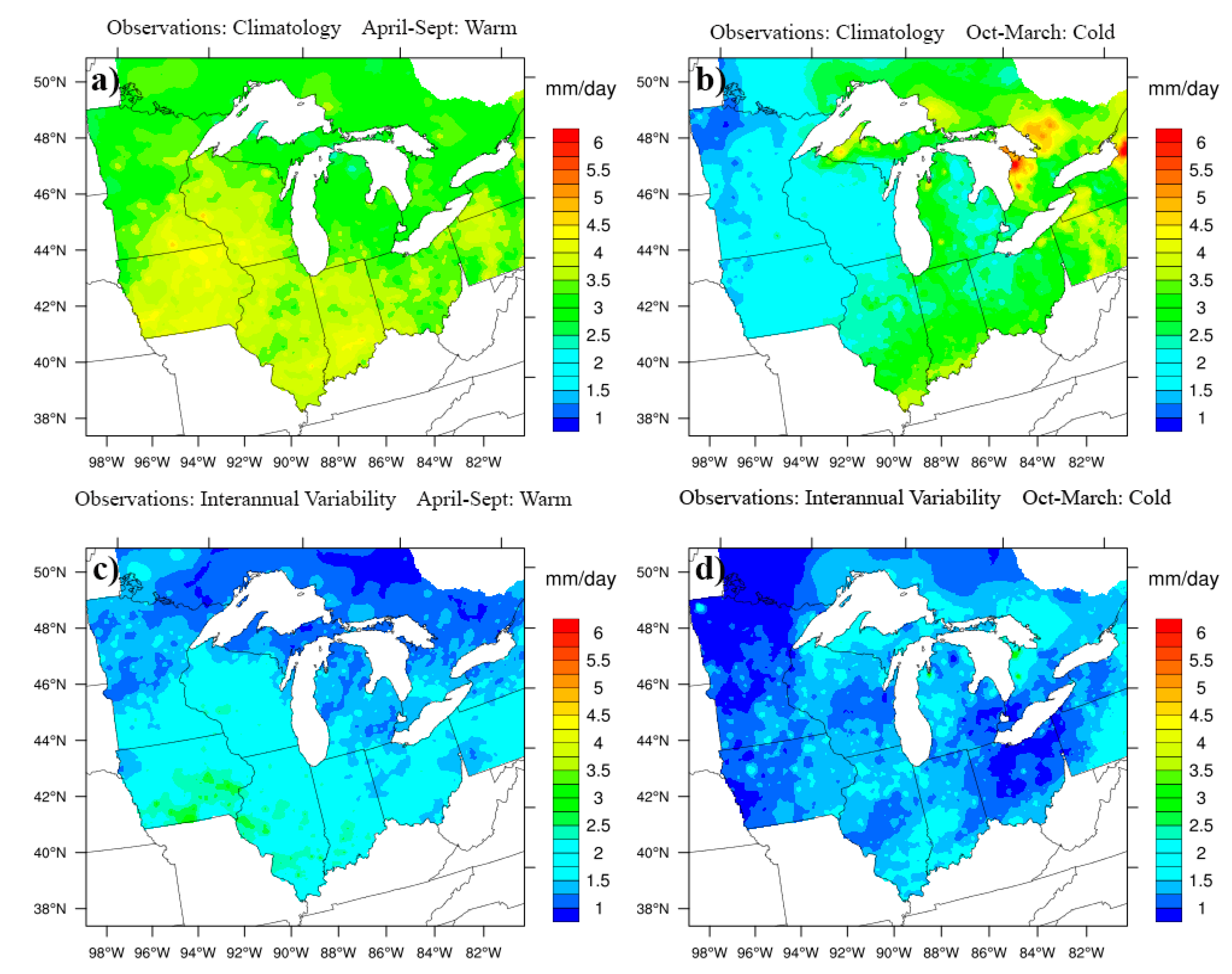
Figure 2 shows seasonal climatology and interannual variability of observed precipitation for 1991 to 2000. For comparison, we defined the warm season from April to September and the cold season from October to March. During the warm season, the Midwest U.S. and Great Lakes region gets ample precipitation as rain mostly used for agriculture production. During the cold season, the temperature drops significantly below freezing. Warm season observations showed an average 4 mm/day precipitation (mostly in the form of rain) in the lower Great Lakes States and reduced precipitation (~3 mm/day) for upper Great lakes U.S. region and lower Canadian provinces (Figure 2a). Indiana, Illinois, Ohio, Wisconsin, and parts of Minnesota showed a relatively higher rainfall in comparison with other U.S. states. Observations showed that with higher precipitation, the interannual variability in the warm season was also higher (2–3 mm/day in wet areas vs. 1 mm/day in drier areas) (Figure 2c). In the cold season, most of the precipitation occurs in the form of snow. Observations showed that the eastern part of the U.S. and Canada had relatively large cold season precipitation in comparison to the western parts of the domain. The average amount of precipitation in the cold season was higher than warm season mostly due to the contribution of lake-effect snow in winters on the east side of the Great Lakes (Figure 2b). Overall, the interannual variability of precipitation for the cold season was lower than that for the warm season. However, the highest interannual variability was found in the same locations that are prone to lake-effect snow.

3.2. NARR Datasets

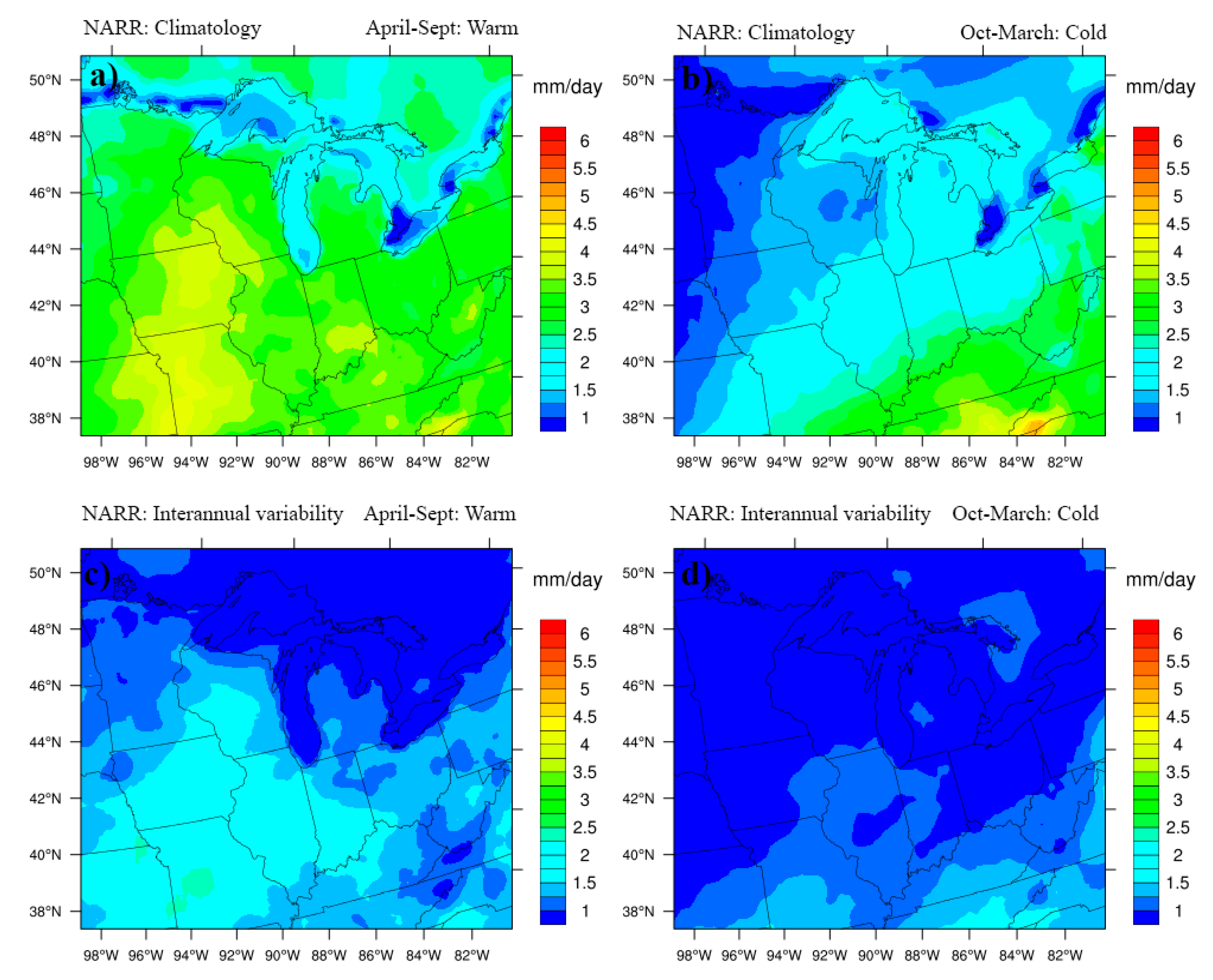
During the warm season, NARR datasets showed a similar climatological trend as observations over the southwest region of the domain (Figure 3a). However, NARR substantially underestimated precipitation over the Great Lakes states. During the cold season, NARR dataset showed a low precipitation bias throughout the domain (Figure 3b). The interannual variability of NARR dataset during the warm season was less than 1 mm/day for northern and around 1.5–2 mm /day in the southern region of the domain (Figure 3c). Note that due to poor resolution (32-km) of NARR data, we also did not observe fine-scale spatial patterns of precipitation. Moreover, the interannual variability of the simulations was also low in the cold season (Figure 3d). Surprisingly, NARR data did not capture lake-effect snow bands observed on the east side of the Lakes in the cold season, resulting in an underprediction of cold-season precipitation in these areas.

3.3. WRF Model Simulations

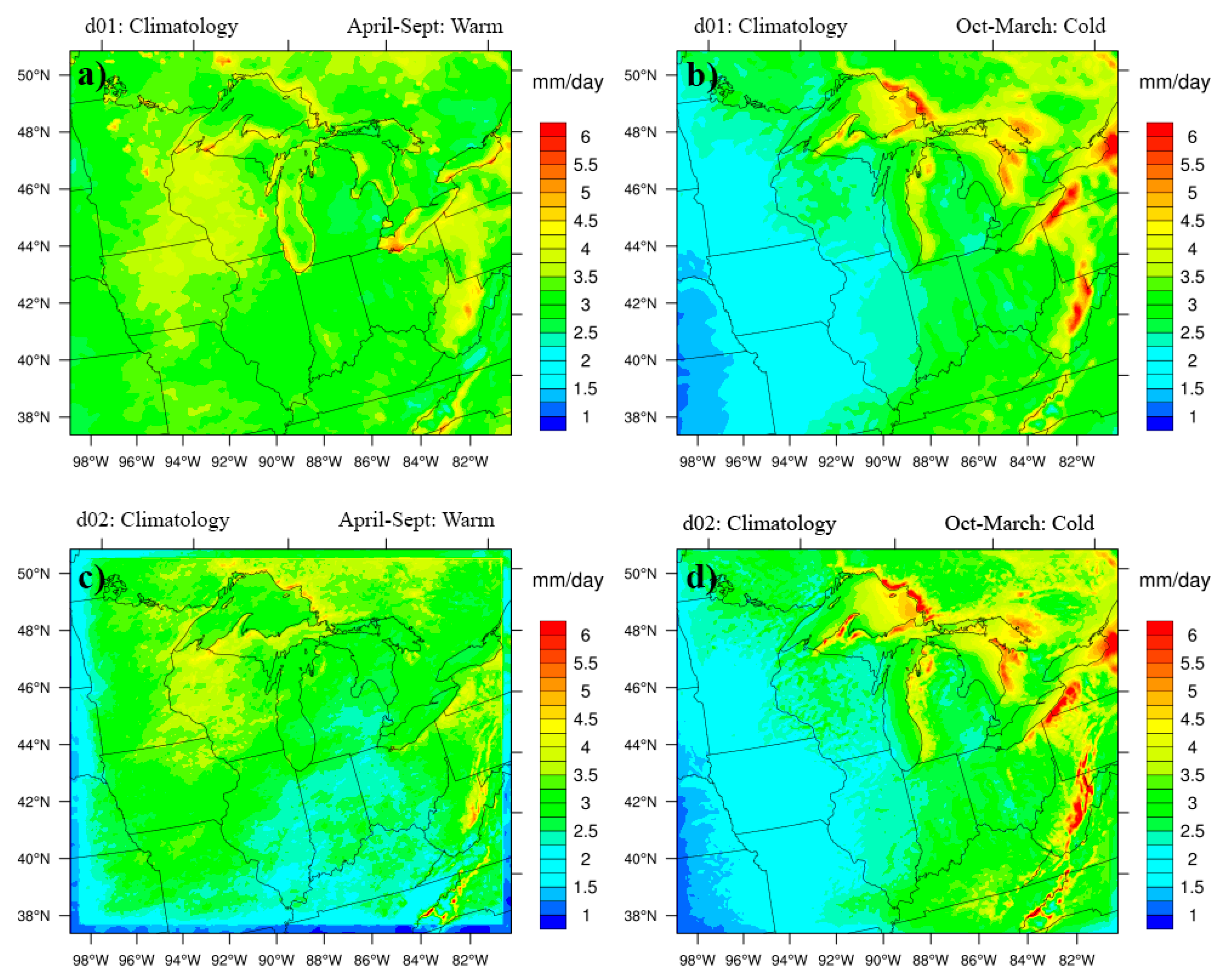
Simulations with the WRF model were performed at 12- and 4-km resolutions for the years 1991 to 2000. Climatological model outputs for the warm and cold season at both 12- and 4-km showed a similar spatial pattern (Figure 4). However, the amounts of precipitation at 4-km were less than at 12-km resolution. Recall that at 12-km resolution, we parameterize the convective precipitation using Kain–Fritsch scheme, while at 4-km we explicitly resolve the convective precipitation. Warm season climatology comparison of WRF simulations (Figure 4a,c) with observations (Figure 2b) suggested that the increase in resolution for our case diminished the warm season precipitation amounts over Wisconsin and Ohio. Both model resolutions also underestimated warm season precipitation amounts (e.g., for Illinois and Indiana). However, during the cold season, WRF showed a good match with observations (Figure 4b,d). The cold season precipitation reached a maximum of 6 mm/day. Interestingly, simulations were able to capture the higher lake-effect precipitation in the east side of the Great Lakes with fine-scale representation at 4-km in comparison to 12-km. The primary reason for the improved capture of lake-effect precipitation was the explicit inclusion of lake surface temperatures as a driver in our model dynamics. As evident, the model outperformed the relatively poor observations in the cold season, as it is difficult to capture the lake-effect processes via observation stations [15]. Both 12- and 4-km simulations captured the seasonal difference in interannual variability (Figure 5). Interannual variability was higher in the warm season (~2 mm/day) and lower in the cold season (~1 mm/day).
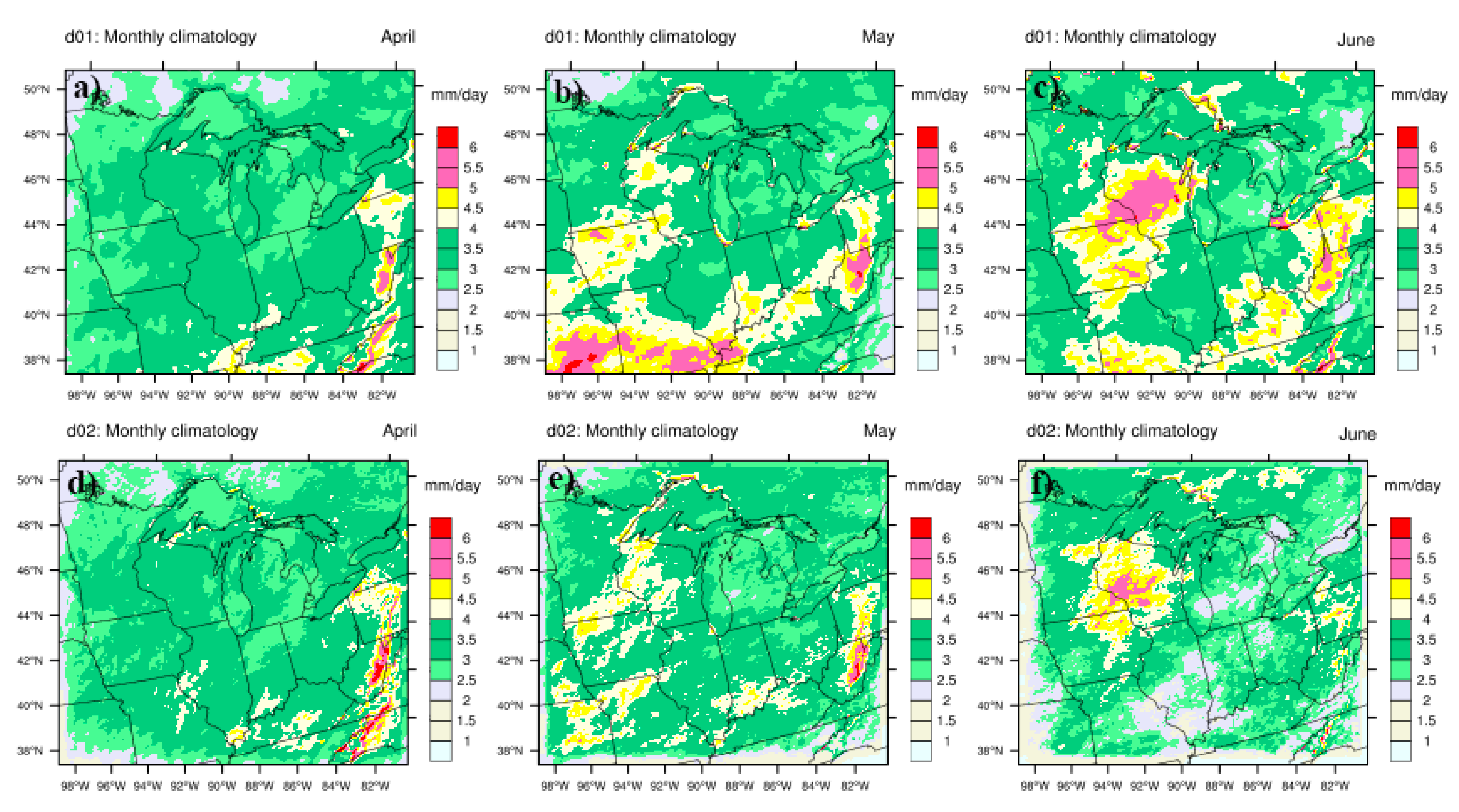
To further explore the differences between the 12-km domain with convective parameterization and the 4 km domain that resolves convection explicitly, we investigated the climatology into monthly parts (Figure 6). In this test, we assessed the monthly climatology for April, May, and June. Both simulations at 12- and 4-km showed almost identical precipitation patterns in April. However, the differences began with large-scale convection occurring in May (Figure 6b,e) and were even more evident in June ((Figure 6c,f). With a higher convective activity, 4-km simulations without explicitly resolving convection did not capture the higher precipitation amounts as evident in observations (Figure 2). This is counter-intuitive to the findings in Sharma and Huang [59] where the grid-scale (i.e., with no parameterized convection) precipitation amounts increased with an increase in resolution for complex mountainous terrain. Thus, an increase in the resolution better captures mechanical/topographic lifting processes in complex terrain but seems to be a disadvantage in capturing convective processes in the relatively flat Midwestern landscape. It is not immediately clear whether these effects are related simply to the need for additional model tuning and calibration at 4-km resolution, or whether physical processes imperfectly captured at 4-km are likely reasons for the low bias in convective precipitation.

3.4. Inter-Comparison among all Datasets

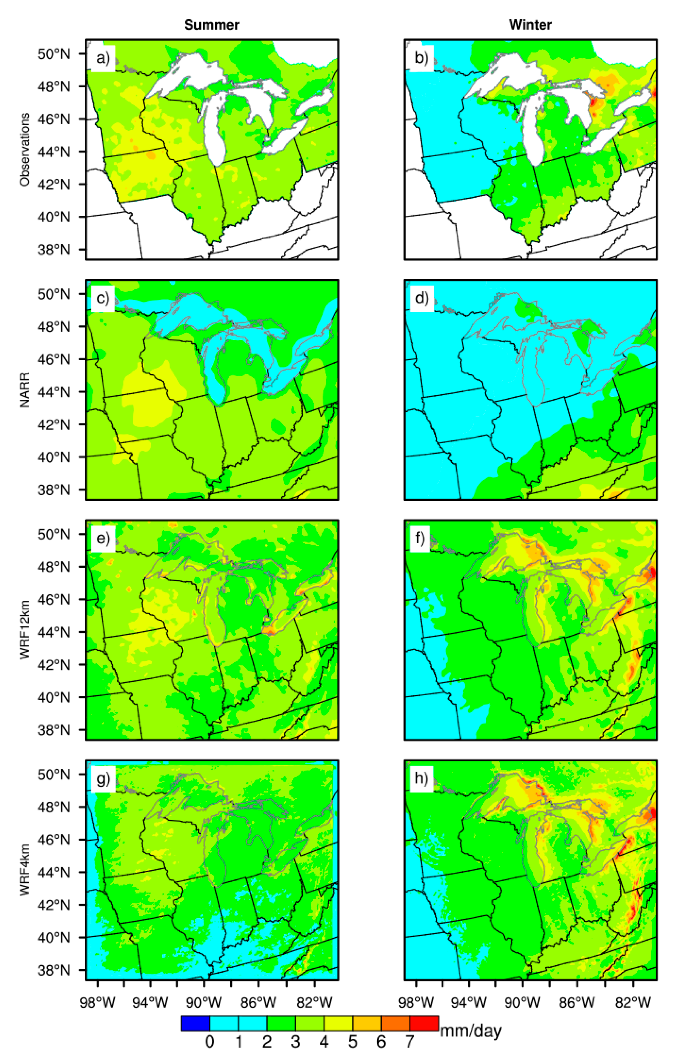
For a detailed comparison between gridded observations, 32-km NARR, and 12- and 4-km WRF model outputs, we plotted summer (June–July–Aug) and winter (Dec–Jan–Feb) average precipitation (Figure 7). During summers, average NARR precipitation compared well with observations for the regions south of the Great Lakes. North of the Great Lakes, observations and simulations matched well for both 12- and 4-km WRF resolutions. However, 4-km as noted earlier showed relatively poor performance in comparison to observations. Interestingly during winters, NARR overall showed poor average precipitation amounts throughout the domain, and both WRF simulations showed comparable results, especially on the eastern side of the Great Lakes (Figure 7b,d,f,h). This suggests that all three models are inheriting these errors primarily from the large-scale forcing. In particular the 4-km likely “inherits” large-scale winter storms from the 12-km simulations. That the large-scale forcing should play an important role makes sense given that winter storms are often large-scale cyclonic events.
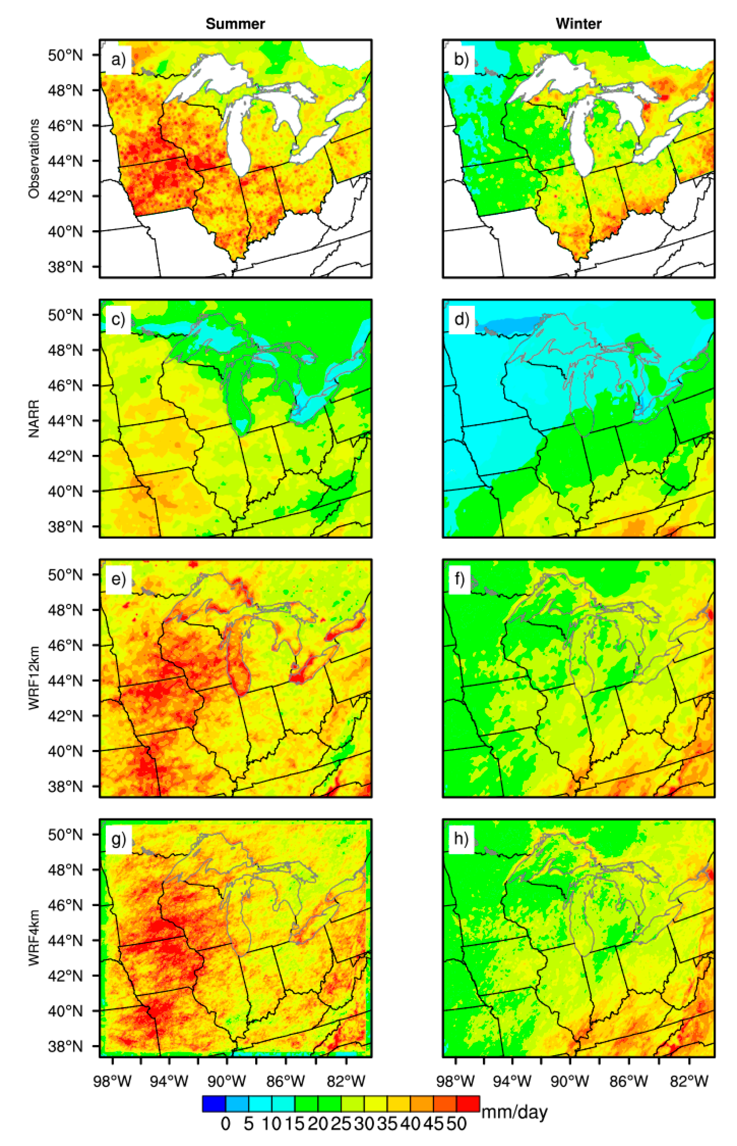
Analysis of 99th percentile extreme daily precipitation (PCP) showed important findings for summer and winter (Figure 8). During summers, NARR showed poor results for PCP, even though it performed well in capturing the mean statistics. This means that extreme storms with high intensity were muted in NARR. However, WRF simulations performed well in comparison with observations for PCP in summers. Interestingly, 4-km WRF simulations that did not show a good match for the mean statistics performed well for the extreme statistics for PCP as shown in Figure 8g. Likewise, WRF PCP at both resolutions also performed well in winters. However, NARR results in PCP underperformed in comparison to observations. The low bias in NARR PCP is to be expected given the scale mismatch between model and observations. That is, event statistics averaged over larger grid scales should show lower values than those observed or simulated at a higher resolution. It is also worth noting that stations often miss extreme storms in summer, so the model underprediction for NARR may be even worse than that shown here.
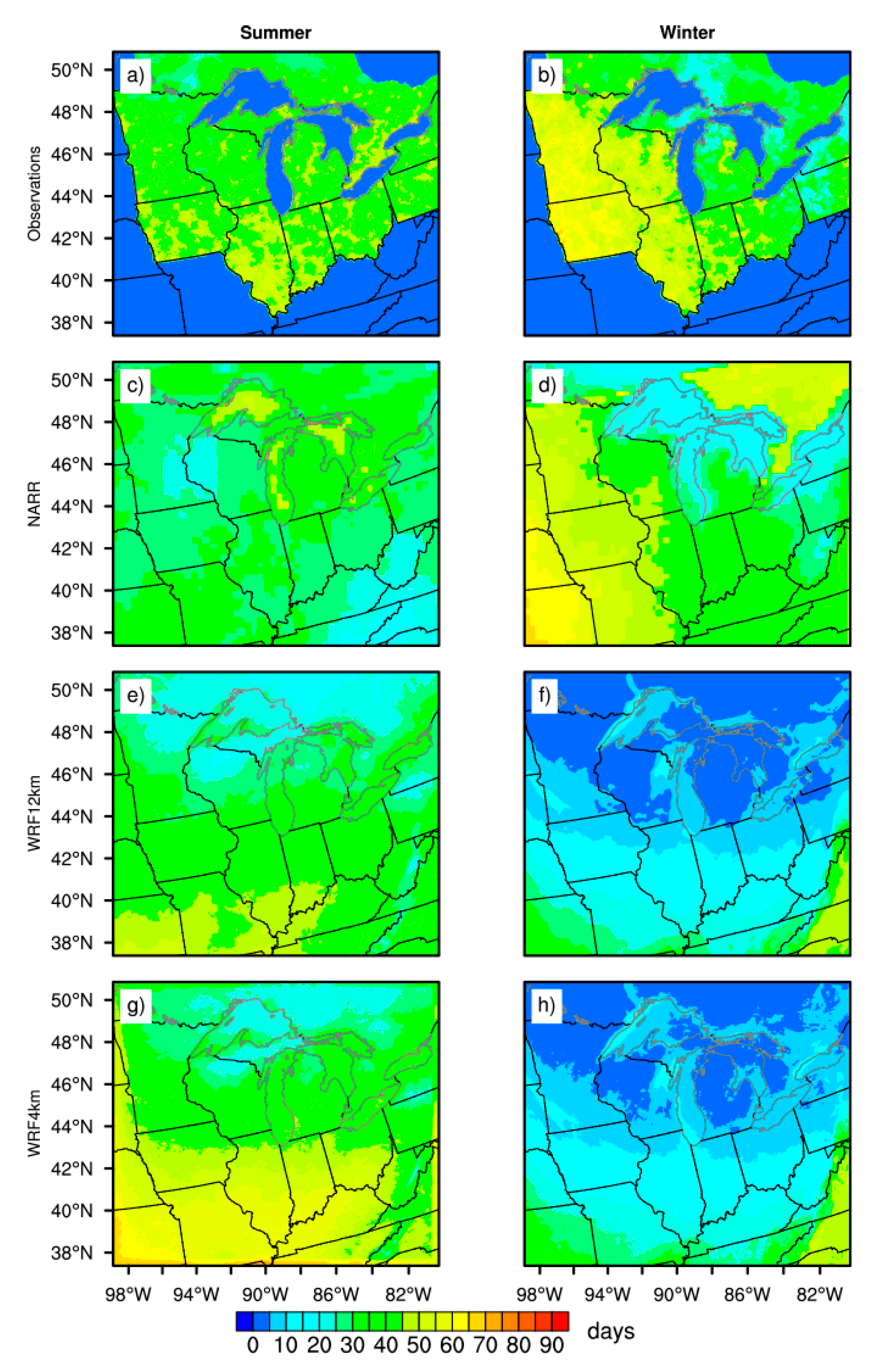
Similarly, we calculated the number of average dry days per year for the 1991–2000 period (Figure 9). During summers, the 4-km WRF simulations performed the best among all products. For example, observations and 4-km output showed a better comparison than other models for Illinois (~65 dry days), Ohio (~50 dry days) and Wisconsin (~40 dry days). Surprisingly, the 4-km simulations did not perform well in reproducing mean climatology statistics for these states. NARR data showed a lesser number of dry days than observations. However, NARR predicted a similar spatial pattern for dry days in the region south of the Great Lakes in winters. NARR again performed poorly for the region north of the Great Lakes showing its weakness in calculating precipitation extremes in winters. WRF models at 12- and 4-km resolutions also underperformed in calculating dry days throughout the domain in winters.
We also compared summer and winter 2-m average daily maximum, mean, and minimum temperatures (refer to Supplementary material). All datasets showed a decreasing trend in temperature with an increasing latitude, as expected. Both NARR and WRF simulations at 12- and 4-km showed a good match with observations for daily maximum and mean temperatures for summers. While WRF simulations well represented the decadal daily average minimum temperatures for summers, the NARR datasets produced 3 deg C higher temperatures for regions south of the Great Lakes (see Figure S1). The wintertime, average daily maximum, mean, and minimum temperatures compared well for all three datasets (see Figure S2). The temperature simulations matched observations better than precipitation in part because the temperature is a prognostic variable rather than a diagnostic variable like precipitation.

4. Discussion and Conclusions

This article investigated the dependence of simulated precipitation and temperature validation on the model type and resolution over a ten-year period from 1991 to 2000. Specifically, NARR data at 32-km resolution and, 12-km and 4-km WRF simulations were compared to gridded observations for the Midwest U.S. and the Great Lakes region for both the warm and cold seasons, and summer and winter seasons. We designed this study with an overarching hypothesis that model performance would improve with an increase in resolution from NARR (32-km) to WRF at 12- and 4-km. Temperature, which is a prognostic variable, and was well captured by all three models. However, we found different strengths and weaknesses related to precipitation for different model formulations.
A detailed evaluation of NARR data for the Great Lakes region showed that it is a useful precipitation product for mean warm season and summer climatological studies, but is extremely poor for winter and cold seasons. One plausible reason for the poor performance for NARR in cold conditions is an inaccurate representation of snow processes and/or data assimilation from observed station datasets that contain an inherent cold-season low bias (snow undercatch). A similar problem with negative precipitation bias was found in observed station datasets, and thus gridded observed stations in this study were bias corrected for precipitation using surface winds (please refer Byun and Hamlet [13] for more details). NARR products, in general, also do not perform well for extreme precipitations, i.e., for both dry days and 99th percentile PCPs. For flood assessment and developing Intensity-Duration-Frequency (IDF) curves, NARR data must not be used for the Great Lakes region. However, NARR data can be used to further downscale for regional and local climate modeling for quiescent summer periods with no convective activity (e.g., a few studies that have successfully used NARR data with such constraints (e.g., [20,24])).
In winter, the NARR showed a strong underprediction of precipitation over most of the inner domain, suggesting too much simulated flow of cold, dry arctic air from the north in winter. These effects could be caused by missing Great Lakes effects in the NARR simulations [15]. Furthermore, it is likely that explicit coupling of a hydrodynamic lake model with an atmospheric model such as WRF can improve the model performance significantly in future projections [15]. The need for such an integrated land-lake-atmosphere modeling system is further exemplified in this study, especially for future climate simulations that lack the lake surface temperatures to drive the regional climate models [82].
In this study, we hypothesized that increasing the model resolution from 12- to 4-km using the WRF model would improve the ability to capture spatial patterns and the intensity of the precipitation. However, the 12-km resolution average seasonal summertime precipitation performed better than the 4-km model. Figure 7 showed that even though the 12-km model outputs drove the 4-km simulations, the 12-km results were superior in reproducing summer precipitation averages in the inner domain, especially during summers. In particular, the 4-km simulations in the southern parts of the domain in Illinois, Indiana, and Ohio showed substantially lower precipitation than observations in summer, and also a substantially larger number of dry days (Figure 9) whereas the 12-km simulations were a closer match with observations. The same underlying issues were present for the 99th percentile extremes shown in Figure 8, however, in this case, the 12-km and 4-km simulations were comparable and showed a similar low bias in the southern parts of the domain. These results demonstrate that the 12- and 4-km simulations are a part of a “grey zone” for which the convective phenomenon is only partly resolved. Both these resolutions are equally capable of capturing strong convective storms in summer that produce extreme precipitation. The results also suggest that the initiation of convective storms and precipitation recycling is weak in the 4-km simulations, resulting in the elevated number of dry days (Figure 9), and low summer precipitation bias for the 4-km simulations in the southern parts of the domain (Figure 7). In summer, however, the results are strongly related to internal dynamics associated with small-scale convective storms, precipitation recycling, interactions with the Great Lakes, etc. Thus, we hypothesize that the poor agreement with observations in summer for the 4-km model is likely due to the problems with convection and weak precipitation recycling. This also explains the inability of our high-resolution WRF model (4-km) without convective parameterization to capture summertime convective precipitation (Figure 6) in comparison with 12-km simulations invoking convective parameterization. Our high-resolution 4-km WRF model simulations captured both extremes, viz., dry days and 99th percentile PCPs. Overall, the difficulty was observed in capturing seasonal precipitation totals and variability. The very close agreement between WRF winter simulations at 12- and 4-km shows the dominant contribution of the large scale forcing in this season.
The 12- and 4-km WRF simulations performed much better in winters, albeit with a substantial wet bias over the western part of the inner domain. In winter, although biased with respect to observations, 12-km and 4-km WRF simulations showed very close agreement for seasonal totals, extremes, and dry days. This was expected, since the storms are typically large-scale events in winter, and the large-scale forcing is in a close agreement between the 12- and 4-km and 12-km runs.
Thus, there may be no need to push for higher resolution for studying convective rainfall. This exercise implies that the parameterization schemes for precipitation are not resolution-independent; thus, a refinement of resolution is no guarantee of a better result. Both WRF model resolutions were able to capture the lake-effect precipitation successfully which was muted/absent in previous studies (e.g., [83,84]). This was due to the inclusion of SST/LST in the WRF model as more accurate lower-boundary surface conditions driving the WRF model that captured the lake effect. At the same time, there need to be considerable efforts to improve numerical model sensitivities to convection, microphysics and the water temperature in simulating winter lake-effect snow [73,85,86,87]. It is beyond the scope of this manuscript to study these aspects.
In conclusion, our study cautions against hastily pushing for increasingly higher resolution in climate studies especially within the “grey zone” around 4-km, and also highlights the need for the careful selection and validation of large-scale boundary forcing data. Alternatively, to avoid the “grey zone,” future studies should use either 10–12 km grid resolution with convective parameterization, or use a very high resolution, say 1-km and explicitly represent the cumulus cloud systems. As mentioned in our experimental design, the choice of the resolution is also dictated by the tradeoffs between computational requirements for large-scale and long-term climate simulations. At the same time, improper validation of input forcing data will also likely produce systematic errors and forced bias correction for one set of simulations may not work for a similar study for a different period or region. We also recognize that the WRF simulations may improve with some form of land data assimilation or longer spin up time (e.g., [20]). We hope to test this hypothesis in future studies. Given our findings, we encourage readers to carefully validate the observed, assimilated, and simulated datasets by validating climatology and extremes before using them for further downscaling and/or impact assessment studies. We hope that lessons from this study will help direct the efforts of researchers to design better-informed climate experiments with improved impact assessments.

Supplementary Materials

The following are available online at https://www.mdpi.com/2073-4433/10/5/266/s1, Figure S1: Left panel shows observed summer 2-m daily maximum average from (a) observations, (d) NARR dataset (g) WRF model output at 12-km, and (j) WRF model output at 4-km for a period of 10 years from year 1991 to 2000. Middle and right panels are same as left, but for mean and minimum temperatures respectively, Figure S2: Same as Figure S1, but for the winter season.

Author Contributions

Conceptualization, A.S., A.F.H., H.J.S.F.; methodology, A.S.; validation, A.S., A.F.H.; formal analysis, A.S., A.F.H.; writing—original draft preparation, A.S.; writing—review and editing, A.S., A.F.H., H.J.S.F.; visualization, A.S.

Funding

This research was supported by the Notre Dame Environmental Change Initiative (ND-ECI) and computing grant from the Great Lakes Consortium for Petascale Computation (GLCPC) for the Blue Waters supercomputers.

Acknowledgments

The research work was supported by the Notre Dame Environmental Change Initiative (ND-ECI). Simulations were performed with NCAR Cheyenne and the National Center for Supercomputing Applications (NCSA) Blue Waters GLCPC computing grants for supercomputing facilities.

Conflicts of Interest

The authors declare no conflict of interest.

References

  1. Gerbush, M.R.; Kristovich, D.A.R.; Laird, N.F. Mesoscale Boundary Layer and Heat Flux Variations over Pack Ice–Covered Lake Erie. J. Appl. Meteorol. Climatol. 2008, 47, 668–682. [Google Scholar] [CrossRef]
  2. Schoof, J. 11. Historical and projected changes in human heat stress in the Midwestern United States. In Climate Change in The Midwest: Impacts, Risks, Vulnerability, And Adaptation; Indiana University Press: Bloomington, IN, USA, 2013; Volume 146, pp. 146–157. [Google Scholar]
  3. Zobel, Z.; Wang, J.; Wuebbles, D.J.; Kotamarthi, V.R. High-resolution dynamical downscaling ensemble projections of future extreme temperature distributions for the United States. Earths Future 2017, 5, 1234–1251. [Google Scholar] [CrossRef]
  4. Zobel, Z.; Wang, J.; Wuebbles, D.J.; Kotamarthi, V.R. Analyses for High-Resolution Projections Through the End of the 21st Century for Precipitation Extremes Over the United States. Earths Future 2018, 6, 1471–1490. [Google Scholar] [CrossRef]
  5. USGCRP. Impacts, Risks, and Adaptation in the United States: Fourth National Climate Assessment; U.S. Global Change Research Program: Washington, DC, USA, 2018; Volume II, p. 1515. Available online: https://nca2018.globalchange.gov/downloads/NCA4_Ch01_Overview.pdf (accessed on 21 April 2019).
  6. Changnon, S.A. Impacts of 1997–98 EI Niño–Generated Weather in the United States. Bull. Am. Meteorol. Soc. 1999, 80, 1819–1828. [Google Scholar] [CrossRef]
  7. Meehl, G.A.; Tebaldi, C. More intense, more frequent, and longer lasting heat waves in the 21st century. Science 2004, 305, 994–997. [Google Scholar] [CrossRef]
  8. Easterling, D.R. Climate Extremes: Observations, Modeling, and Impacts. Science 2000, 289, 2068–2074. [Google Scholar] [CrossRef] [Green Version]
  9. Wuebbles, D.; Cardinale, B.; Cherkauer, K.; Davidson-Arnott, R.; Hellmann, J.J.; Infante, D.; Johnson, L.; de Loe, R.; Lofgren, B.; Packman, A.; et al. An Assessment of the Impacts of Climate Change on the Great Lakes; The Environmental Law & Policy Center: Chicago, IL, USA, 2019; Available online: http://elpc.org/glclimatechange/ (accessed on 21 April 2019).
  10. Carpenter, S.R.; Booth, E.G.; Kucharik, C.J. Extreme precipitation and phosphorus loads from two agricultural watersheds. Limnol. Oceanogr. 2018, 63, 1221–1233. [Google Scholar] [CrossRef]
  11. Kelly, S.A.; Takbiri, Z.; Belmont, P.; Foufoula-Georgiou, E. Human amplified changes in precipitation–runoff patterns in large river basins of the Midwestern United States. Hydrol. Earth Syst. Sci. 2017, 21, 5065–5088. [Google Scholar] [CrossRef] [Green Version]
  12. USGCRP. Climate Science Special Report: Fourth National Climate Assessment; U.S. Global Change Research Program: Washington, DC, USA, 2017; Volume I, p. 475.
  13. Byun, K.; Hamlet, A.F. Projected changes in future climate over the Midwest and Great Lakes region using downscaled CMIP5 ensembles. Int. J. Climatol. 2018, 38, e531–e553. [Google Scholar] [CrossRef]
  14. Intergovernmental Panel on Climate Change. Climate Change 2007—The Physical Science Basis: Working Group I Contribution to the Fourth Assessment Report of the IPCC; Cambridge University Press: Cambridge, UK, 2007; ISBN 9780521880091. [Google Scholar]
  15. Sharma, A.; Hamlet, A.F.; Fernando, H.J.S.; Catlett, C.E.; Horton, D.E.; Kotamarthi, V.R.; Kristovich, D.A.R.; Packman, A.I.; Tank, J.L.; Wuebbles, D.J. The Need for an Integrated Land-Lake-Atmosphere Modeling System, Exemplified by North America’s Great Lakes Region. Earths Future 2018, 6, 1366–1379. [Google Scholar] [CrossRef]
  16. Byun, K.; Chiu, C.-M.; Hamlet, A.F. Effects of 21st century climate change on seasonal flow regimes and hydrologic extremes over the Midwest and Great Lakes region of the US. Sci. Total Environ. 2019, 650, 1261–1277. [Google Scholar] [CrossRef]
  17. Hamlet, A.F.; Chiu, C.M.; Sharma, A.; Byun, K.; Hanson, Z. Developing Flexible, Integrated Hydrologic Modeling Systems for Multiscale Analysis in the Midwest and Great Lakes Region. In Proceedings of the AGU Fall Meeting, San Francisco, CA, USA, 12–16 December 2016. [Google Scholar]
  18. Keeley, M.; Koburger, A.; Dolowitz, D.P.; Medearis, D.; Nickel, D.; Shuster, W. Perspectives on the use of green infrastructure for stormwater management in Cleveland and Milwaukee. Environ. Manage. 2013, 51, 1093–1108. [Google Scholar] [CrossRef]
  19. Sharma, A.; Conry, P.; Fernando, H.J.S.; Hamlet, A.F.; Hellmann, J.J.; Chen, F. Green and cool roofs to mitigate urban heat island effects in the Chicago metropolitan area: Evaluation with a regional climate model. Environ. Res. Lett. 2016, 11, 064004. [Google Scholar] [CrossRef]
  20. Sharma, A.; Fernando, H.J.S.; Hamlet, A.F.; Hellmann, J.J.; Barlage, M.; Chen, F. Urban meteorological modeling using WRF: A sensitivity study. Int. J. Climatol. 2017, 37, 1885–1900. [Google Scholar] [CrossRef]
  21. Sharma, A.; Woodruff, S.; Budhathoki, M.; Hamlet, A.F.; Chen, F.; Fernando, H.J.S. Role of green roofs in reducing heat stress in vulnerable urban communities—A multidisciplinary approach. Environ. Res. Lett. 2018, 13, 094011. [Google Scholar] [CrossRef]
  22. Sharma, A.; Fernando, H.J.S.; Hellmann, J.; Chen, F. Sensitivity of WRF Model to Urban Parameterizations, With Applications to Chicago Metropolitan Urban Heat Island. In Proceedings of the ASME 2014 4th Joint US-European Fluids Engineering Division Summer Meeting collocated with the ASME 2014 12th International Conference on Nanochannels, Microchannels, and Minichannels, Chicago, IL, USA, 3–7 August 2014. [Google Scholar]
  23. Conry, P.; Fernando, H.J.S.; Leo, L.S.; Sharma, A.; Potosnak, M.; Hellmann, J. Multi-Scale Simulations of Climate-Change Influence on Chicago Heat Island. In Proceedings of the ASME 2014 4th Joint US-European Fluids Engineering Division Summer Meeting collocated with the ASME 2014 12th International Conference on Nanochannels, Microchannels, and Minichannels, Chicago, IL, USA, 3–7 August 2014. [Google Scholar]
  24. Conry, P.; Sharma, A.; Potosnak, M.J.; Leo, L.S.; Bensman, E.; Hellmann, J.J.; Fernando, H.J.S. Chicago’s heat island and climate change: Bridging the scales via dynamical downscaling. J. Appl. Meteorol. Climatol. 2015, 54, 1430–1448. [Google Scholar] [CrossRef]
  25. Silva, M.P.; Sharma, A.; Budhathoki, M.; Jain, R.; Catlett, C.E. Neighborhood scale heat mitigation strategies using Array of Things (AoT) data in Chicago. In Proceedings of the AGU Fall Meeting, Washington, DC, USA, 10–14 December 2018. [Google Scholar]
  26. Sharma, A.; Woodruff, S.; Budhathoki, M.; Hamlet, A.F.; Fernando, H.J.S.; Chen, F. Can green roofs reduce urban heat stress in vulnerable urban communities: A coupled atmospheric and social modeling approach. In Proceedings of the AGU Fall Meeting, New Orleans, LA, USA, 11–15 December 2017. [Google Scholar]
  27. Bunnell, D.B.; Barbiero, R.P.; Ludsin, S.A.; Madenjian, C.P.; Warren, G.J.; Dolan, D.M.; Brenden, T.O.; Briland, R.; Gorman, O.T.; He, J.X.; et al. Changing Ecosystem Dynamics in the Laurentian Great Lakes: Bottom-Up and Top-Down Regulation. Bioscience 2014, 64, 26–39. [Google Scholar] [CrossRef]
  28. Goodspeed, R.; Riseng, C.; Wehrly, K.; Yin, W.; Mason, L.; Schoenfeldt, B. Applying design thinking methods to ecosystem management tools: Creating the Great Lakes Aquatic Habitat Explorer. Mar. Policy 2016, 69, 134–145. [Google Scholar] [CrossRef]
  29. Lubchenco, J.; Sutley, N. Proposed U.S. Policy for Ocean, Coast, and Great Lakes Stewardship. Science 2010, 328, 1485–1486. [Google Scholar] [CrossRef]
  30. Sierszen, M.E.; Morrice, J.A.; Trebitz, A.S.; Hoffman, J.C. A review of selected ecosystem services provided by coastal wetlands of the Laurentian Great Lakes. Aquat. Ecosyst. Health Manag. 2012, 15, 92–106. [Google Scholar] [CrossRef]
  31. Mueller, N.D.; Butler, E.E.; McKinnon, K.A.; Rhines, A.; Tingley, M.; Holbrook, N.M.; Huybers, P. Cooling of US Midwest summer temperature extremes from cropland intensification. Nat. Clim. Chang. 2015, 6, 317. [Google Scholar] [CrossRef]
  32. Goswami, B.B.; Mukhopadhyay, P.; Khairoutdinov, M.; Goswami, B.N. Simulation of Indian summer monsoon intraseasonal oscillations in a superparameterized coupled climate model: need to improve the embedded cloud resolving model. Clim. Dyn. 2013, 41, 1497–1507. [Google Scholar] [CrossRef]
  33. Wehner, M.F.; Smith, R.L.; Bala, G.; Duffy, P. The effect of horizontal resolution on simulation of very extreme US precipitation events in a global atmosphere model. Clim. Dyn. 2010, 34, 241–247. [Google Scholar] [CrossRef]
  34. Kendon, E.J.; Roberts, N.M.; Senior, C.A.; Roberts, M.J. Realism of Rainfall in a Very High-Resolution Regional Climate Model. J. Clim. 2012, 25, 5791–5806. [Google Scholar] [CrossRef]
  35. Bukovsky, M.S.; Karoly, D.J. A Regional Modeling Study of Climate Change Impacts on Warm-Season Precipitation in the Central United States. J. Clim. 2011, 24, 1985–2002. [Google Scholar] [CrossRef]
  36. Parmesan, C.; Root, T.L.; Willig, M.R. Impacts of Extreme Weather and Climate on Terrestrial Biota. Bull. Am. Meteorol. Soc. 2000, 81, 443–450. [Google Scholar] [CrossRef]
  37. Parmesan, C.; Martens, P. Climate change, wildlife, and human health. Biodiversity Change and Human Health: From Ecosystem Services to Spread of Disease. 2009, 69, 245–266. [Google Scholar]
  38. Castro, C.L.; Pielke, R.A., Sr. Dynamical downscaling: Assessment of value retained and added using the Regional Atmospheric Modeling System (RAMS). J. Geophys. Res. 2005. [Google Scholar] [CrossRef]
  39. Pielke, R.A., Sr.; Wilby, R.L. Regional climate downscaling: What’s the point? Eos Trans. AGU 2012, 93, 52–53. [Google Scholar] [CrossRef]
  40. Pielke, R. Comments on “The North American Regional Climate Change Assessment Program: Overview of Phase I Results”. Bull. Am. Meteorol. Soc. 2013, 94, 1075–1077. [Google Scholar] [CrossRef] [Green Version]
  41. Mearns, L.O.; Bukovsky, M.S.; Leung, R.; Qian, Y.; Arritt, R.; Gutowski, W.; Takle, E.S.; Biner, S.; Caya, D.; Correia, J.; et al. Reply to “Comments on ‘The North American Regional Climate Change Assessment Program: Overview of Phase I Results’”. Bull. Am. Meteorol. Soc. 2013, 94, 1077–1078. [Google Scholar] [CrossRef]
  42. Rockel, B.; Castro, C.L.; Pielke, R.A., Sr.; von Storch, H.; Leoncini, G. Dynamical downscaling: Assessment of model system dependent retained and added variability for two different regional climate models. J. Geophys. Res. 2008, 113, D05108. [Google Scholar] [CrossRef]
  43. Wang, J.; Kotamarthi, V.R. Assessment of Dynamical Downscaling in Near-Surface Fields with Different Spectral Nudging Approaches Using the Nested Regional Climate Model (NRCM). J. Appl. Meteorol. Climatol. 2013, 52, 1576–1591. [Google Scholar] [CrossRef]
  44. Pielke, R.A. A Recommended Specific Definition of “Resolution”. Bull. Am. Meteorol. Soc. 1991, 72, 1914. [Google Scholar] [CrossRef]
  45. Pielke, R.A. Further Comments on “The Differentiation between Grid Spacing and Resolution and Their Application to Numerical Modeling”. Bull. Am. Meteorol. Soc. 2001, 82, 699–700. [Google Scholar] [CrossRef] [Green Version]
  46. Laprise, R. The resolution of global spectral models. Bull. Am. Meteorol. Soc. 1992, 73, 1453–1455. [Google Scholar] [CrossRef]
  47. Pielke, R.A., Sr. Mesoscale Meteorological Modeling; Academic Press: Cambridge, MA, USA, 2013; ISBN 9780123852380. [Google Scholar]
  48. Kalnay, E.; Kanamitsu, M.; Kistler, R.; Collins, W.; Deaven, D.; Gandin, L.; Iredell, M.; Saha, S.; White, G.; Woollen, J.; et al. The NCEP/NCAR 40-Year Reanalysis Project. Bull. Am. Meteorol. Soc. 1996, 77, 437–472. [Google Scholar] [CrossRef]
  49. Maurer, E.P.; Wood, A.W.; Adam, J.C.; Lettenmaier, D.P.; Nijssen, B. A Long-Term Hydrologically Based Dataset of Land Surface Fluxes and States for the Conterminous United States. J. Clim. 2002, 15, 3237–3251. [Google Scholar] [CrossRef]
  50. Hamlet, A.F.; Lettenmaier, D.P. Production of Temporally Consistent Gridded Precipitation and Temperature Fields for the Continental United States. J. Hydrometeorol. 2005, 6, 330–336. [Google Scholar] [CrossRef]
  51. Shepard, D.S. Computer Mapping: The SYMAP Interpolation Algorithm. Spat. Stat. Models 1984, 40, 133–145. [Google Scholar]
  52. World Meteorological Organization. Guide to Meteorological Instruments and Methods of Observation; Secretariat of the World Meteorological Organization: Geneva, Switzerland, 1983. [Google Scholar]
  53. Yang, D.; Goodison, B.E.; Metcalfe, J.R.; Golubev, V.S.; Bates, R.; Pangburn, T.; Hanson, C.L. Accuracy of NWS 8″ Standard Nonrecording Precipitation Gauge: Results and Application of WMO Intercomparison. J. Atmos. Ocean. Technol. 1998, 15, 54–68. [Google Scholar] [CrossRef]
  54. Mekis, É.; Vincent, L.A. An Overview of the Second Generation Adjusted Daily Precipitation Dataset for Trend Analysis in Canada. Atmosphere Ocean 2011, 49, 163–177. [Google Scholar] [CrossRef] [Green Version]
  55. Mesinger, F.; DiMego, G.; Kalnay, E.; Mitchell, K.; Shafran, P.C.; Ebisuzaki, W.; Jović, D.; Woollen, J.; Rogers, E.; Berbery, E.H.; et al. North American Regional Reanalysis. Bull. Am. Meteorol. Soc. 2006, 87, 343–360. [Google Scholar] [CrossRef] [Green Version]
  56. Lo, J.C.-F.; Yang, Z.-L.; Pielke, R.A., Sr. Assessment of three dynamical climate downscaling methods using the Weather Research and Forecasting (WRF) model. J. Geophys. Res. 2008, 113, 1306. [Google Scholar] [CrossRef]
  57. Skamarock, W.C.; Klemp, J.B.; Dudhia, J.; Gill, D.O.; Barker, D.M.; Wang, W.; Powers, J.G. A Description of the Advanced Research WRF Version 2. 2005. Available online: http://opensky.ucar.edu/islandora/object/technotes:479 (accessed on 21 April 2019).
  58. Heikkilä, U.; Sandvik, A.; Sorteberg, A. Dynamical downscaling of ERA-40 in complex terrain using the WRF regional climate model. Clim. Dyn. 2011, 37, 1551–1564. [Google Scholar] [CrossRef]
  59. Sharma, A.; Huang, H.-P. Regional Climate Simulation for Arizona: Impact of Resolution on Precipitation. Adv. Meteorol. 2012, 2012, 505726. [Google Scholar] [CrossRef]
  60. Talbot, C.; Bou-Zeid, E.; Smith, J. Nested Mesoscale Large-Eddy Simulations with WRF: Performance in Real Test Cases. J. Hydrometeorol. 2012, 13, 1421–1441. [Google Scholar] [CrossRef]
  61. Pithani, P.; Ghude, S.D.; Chennu, V.N.; Kulkarni, R.G.; Steeneveld, G.-J.; Sharma, A.; Prabhakaran, T.; Chate, D.M.; Gultepe, I.; Jenamani, R.K.; et al. WRF Model Prediction of a Dense Fog Event Occurred During the Winter Fog Experiment (WIFEX). Pure Appl. Geophys. 2018, 176. [Google Scholar] [CrossRef]
  62. Sharma, A.; Huang, H.-P.; Zavialov, P.; Khan, V. Impact of Desiccation of Aral Sea on the Regional Climate of Central Asia Using WRF Model. Pure Appl. Geophys. 2018, 175, 465–478. [Google Scholar] [CrossRef]
  63. Conry, P.; Sharma, A.; Leo, L.; Fernando, H.J.S.; Potosnak, M.; Hellmann, J. Modeling and measuring neighborhood scale flow, turbulence, and temperature within Chicago heat island. In Proceedings of the APS Division of Fluid Dynamics Meeting, Pittsburgh, PA, USA, 24–26 November 2013. [Google Scholar]
  64. Kanamitsu, M.; Ebisuzaki, W.; Woollen, J.; Yang, S.-K.; Hnilo, J.J.; Fiorino, M.; Potter, G.L. NCEP-DOE Amip-II Reanalysis (R-2). Bull. Am. Meteorol. Soc. 2002, 83, 1631–1644. [Google Scholar] [CrossRef]
  65. Fry, J.; Xian, G.Z.; Jin, S.; Dewitz, J.; Homer, C.G.; Yang, L.; Barnes, C.A.; Herold, N.D.; Wickham, J.D. Completion of the 2006 national land cover database for the conterminous United States. Photogramm. Eng. Remote Sens. 2011, 77, 858–864. [Google Scholar]
  66. Hong, S.-Y.; Lim, J.-O.J. The WRF single-moment 6-class microphysics scheme (WSM6). Asia Pac. J. Atmos. Sci. 2006, 42, 129–151. [Google Scholar]
  67. Dudhia, J. Numerical Study of Convection Observed during the Winter Monsoon Experiment Using a Mesoscale Two-Dimensional Model. J. Atmos. Sci. 1989, 46, 3077–3107. [Google Scholar] [CrossRef] [Green Version]
  68. Mlawer, E.J.; Taubman, S.J.; Brown, P.D.; Iacono, M.J.; Clough, S.A. Radiative transfer for inhomogeneous atmospheres: RRTM, a validated correlated-k model for the longwave. J. Geophys. Res. Atmos. 1997, 102, 16663–16682. [Google Scholar] [CrossRef] [Green Version]
  69. Noh, Y.; Cheon, W.G.; Hong, S.Y.; Raasch, S. Improvement of the K-profile Model for the Planetary Boundary Layer based on Large Eddy Simulation Data. Bound. Layer Meteorol. 2003, 107, 401–427. [Google Scholar] [CrossRef]
  70. Chen, F.; Dudhia, J. Coupling an Advanced Land Surface–Hydrology Model with the Penn State–NCAR MM5 Modeling System. Part I: Model Implementation and Sensitivity. Mon. Weather Rev. 2001, 129, 569–585. [Google Scholar] [CrossRef]
  71. Kain, J.S. The Kain–Fritsch Convective Parameterization: An Update. J. Appl. Meteorol. 2004, 43, 170–181. [Google Scholar] [CrossRef]
  72. Xiao, C.; Lofgren, B.M.; Wang, J. Improving the lake scheme within a coupled WRF-lake model in the Laurentian Great Lakes. JAMES 2016, 11. [Google Scholar] [CrossRef]
  73. Theeuwes, N.E.; Steeneveld, G.J.; Krikken, F.; Holtslag, A.A.M. Mesoscale modeling of lake effect snow over Lake Erie - sensitivity to convection, microphysics and the water temperature. Adv. Sci. Res. 2010, 2010, 15–22. [Google Scholar] [CrossRef]
  74. Campbell, L.S.; Steenburgh, W.J. The OWLeS IOP2b Lake-Effect Snowstorm: Mechanisms Contributing to the Tug Hill Precipitation Maximum. Mon. Weather Rev. 2017, 145, 2461–2478. [Google Scholar] [CrossRef]
  75. McMillen, J.D.; Steenburgh, W.J. Capabilities and Limitations of Convection-Permitting WRF Simulations of Lake-Effect Systems over the Great Salt Lake. Weather Forecast. 2015, 30, 1711–1731. [Google Scholar] [CrossRef]
  76. Pan, Z.; Takle, E.; Gutowski, W.; Turner, R. Long Simulation of Regional Climate as a Sequence of Short Segments. Mon. Weather Rev. 1999, 127, 308–321. [Google Scholar] [CrossRef] [Green Version]
  77. Conil, S.; Hall, A. Local Regimes of Atmospheric Variability: A Case Study of Southern California. J. Clim. 2006, 19, 4308–4325. [Google Scholar] [CrossRef]
  78. Qian, J.-H.; Seth, A.; Zebiak, S. Reinitialized versus Continuous Simulations for Regional Climate Downscaling. Mon. Weather Rev. 2003, 131, 2857–2874. [Google Scholar] [CrossRef]
  79. Žagar, N.; Žagar, M.; Cedilnik, J.; Gregorič, G.; Rakovec, J. Validation of mesoscale low-level winds obtained by dynamical downscaling of ERA40 over complex terrain. Tellus Ser. A Dyn. Meteorol. Oceanogr. 2006, 58, 445–455. [Google Scholar] [CrossRef] [Green Version]
  80. Jiménez, P.A.; Fidel González-Rouco, J.; García-Bustamante, E.; Navarro, J.; Montávez, J.P.; de Arellano, J.V.-G.; Dudhia, J.; Muñoz-Roldan, A. Surface Wind Regionalization over Complex Terrain: Evaluation and Analysis of a High-Resolution WRF Simulation. J. Appl. Meteorol. Climatol. 2010, 49, 268–287. [Google Scholar] [CrossRef] [Green Version]
  81. Lucas-Picher, P.; Boberg, F.; Christensen, J.H.; Berg, P. Dynamical Downscaling with Reinitializations: A Method to Generate Finescale Climate Datasets Suitable for Impact Studies. J. Hydrometeorol. 2013, 14, 1159–1174. [Google Scholar] [CrossRef]
  82. Winkler, J.A.; Arritt, R.W.; Pryor, S.C. Climate Projections for the Midwest: Availability, Interpretation and Synthesis. US National Climate Assessment Midwest Technical Input Report. 2012. Available online: http://glisa.umich.edu/media/files/NCA/MTIT_Future.pdf (accessed on 21 April 2019).
  83. Rasmussen, R.; Ikeda, K.; Liu, C.; Gochis, D.; Chen, F.; Barlage, M.J.; Dai, A.; Dudhia, J.; Clark, M.P.; Gutmann, E.D.; et al. High Resolution Climate Modeling of the Water Cycle over the Contiguous United States Including Potential Climate Change Scenarios. 2015. Available online: https://www.gewexevents.org/wp-content/uploads/Rasmussen_CONUS_USRHP2016.pdf (accessed on 21 April 2019).
  84. Liu, C.; Ikeda, K.; Rasmussen, R.; Barlage, M.; Newman, A.J.; Prein, A.F.; Chen, F.; Chen, L.; Clark, M.; Dai, A.; et al. Continental-scale convection-permitting modeling of the current and future climate of North America. Clim. Dyn. 2017, 49, 71–95. [Google Scholar] [CrossRef]
  85. Schroeder, J.J.; Kristovich, D.A.R.; Hjelmfelt, M.R. Boundary Layer and Microphysical Influences of Natural Cloud Seeding on a Lake-Effect Snowstorm. Mon. Weather Rev. 2006, 134, 1842–1858. [Google Scholar] [CrossRef]
  86. Kristovich, D.A.R.; Clark, R.D.; Frame, J.; Geerts, B.; Knupp, K.R.; Kosiba, K.A.; Laird, N.F.; Metz, N.D.; Minder, J.R.; Sikora, T.D.; et al. The Ontario Winter Lake-Effect Systems Field Campaign: Scientific and Educational Adventures to Further Our Knowledge and Prediction of Lake-Effect Storms. Bull. Am. Meteorol. Soc. 2017, 98, 315–332. [Google Scholar] [CrossRef]
  87. Field, P.R.; Brožková, R.; Chen, M.; Dudhia, J.; Lac, C.; Hara, T.; Honnert, R.; Olson, J.; Siebesma, P.; de Roode, S.; et al. Exploring the convective grey zone with regional simulations of a cold air outbreak. Q.J.R. Meteorol. Soc. 2017, 143, 2537–2555. [Google Scholar] [CrossRef]
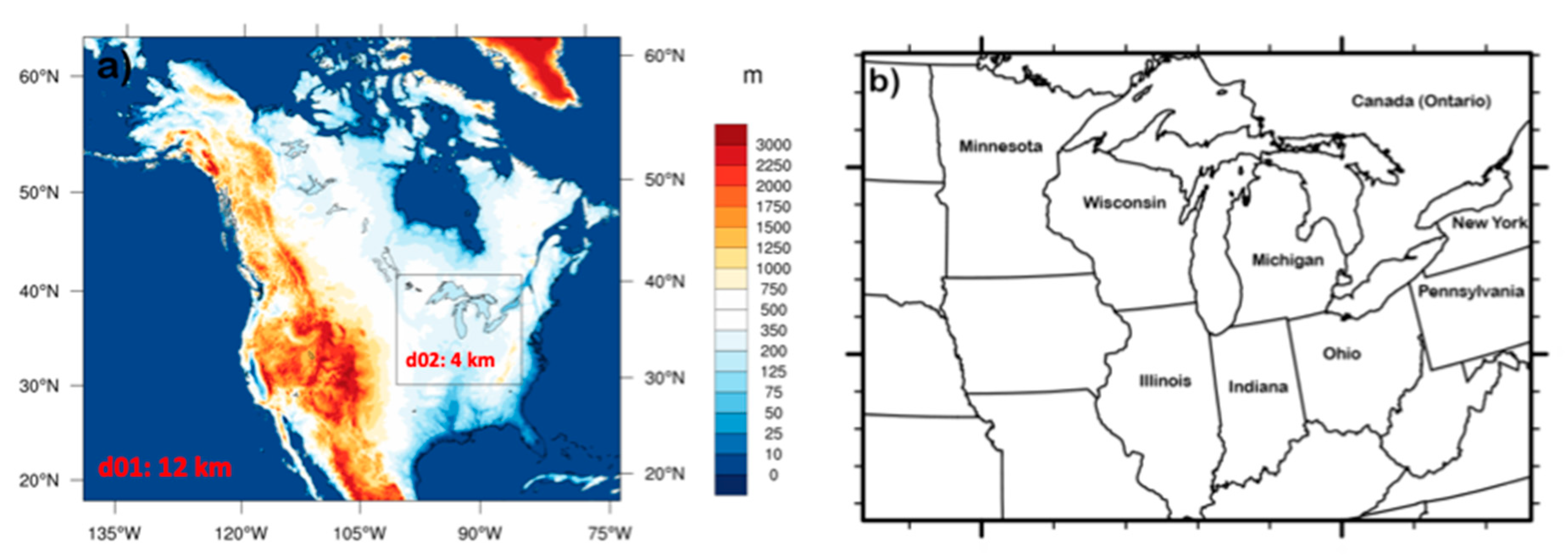
Figure 1. (a) Two-way nested domains for the Weather Research and Forecasting model (WRF) model with a grid size of 12- and 4-km as d01 and d02 respectively, overlaid on a terrain height map; and (b) a map showing the states in the U.S. and Canadian province Ontario surrounding the Great Lakes.
Atmosphere 10 00266 g001
Figure 2. Seasonal climatology of observed gridded precipitation for (a) warm season from April–September and (b) cold season from October to March for a period of 10 years from the year 1991 to 2000. Similarly, seasonal interannual variability of observed precipitation for (c) warm and (d) cold season.
Atmosphere 10 00266 g002
Figure 3. Same as Figure 2 but for North American Regional Reanalysis (NARR) data.
Atmosphere 10 00266 g003
Figure 4. Seasonal climatology of simulated WRF model precipitation for domain at 12-km for (a) warm and (b) cold season for a period of 10 years from the year 1991 to 2000. Panels (c) and (d) are the same as (a) and (b) but for domain at 4-km.
Atmosphere 10 00266 g004
Figure 5. Same as Figure 4 but for interannual variability of simulated WRF model precipitation.
Atmosphere 10 00266 g005
Figure 6. Top panel shows the monthly climatological precipitation for WRF model domain at 12-km with explicitly resolve convective precipitation for (a) April, (b) May, and (June). Bottom panel (df) are same as top panel (ac) respectively but for domain at 4-km without explicit resolved convection.
Atmosphere 10 00266 g006
Figure 7. Left panel shows summer (June–July–Aug) average precipitation for a period of 10 years from the year 1991 to 2000 from (a) observations, (c) NARR dataset (e) WRF model output at 12-km, and (g) WRF model output at 4-km. The right panel (b,d,f,h) is the same as left, but for winter (Dec–Jan–Feb).
Atmosphere 10 00266 g007
Figure 8. Same as Figure 7, but for 99th percentile extreme daily precipitation (PCP).
Atmosphere 10 00266 g008
Figure 9. Same as Figure 7, but for the average number of dry days per year.
Atmosphere 10 00266 g009