Article

The South Atlantic–South Indian Ocean Pattern: a Zonally Oriented Teleconnection along the Southern Hemisphere Westerly Jet in Austral Summer

State Key Laboratory of Numerical Modeling for Atmospheric Sciences and Geophysical Fluid Dynamics, Institute of Atmospheric Physics, Chinese Academy of Sciences, Beijing 100029, China
Atmosphere 2019, 10(5), 259; https://doi.org/10.3390/atmos10050259
Submission received: 11 April 2019 / Revised: 6 May 2019 / Accepted: 7 May 2019 / Published: 9 May 2019
(This article belongs to the Section Meteorology)

Abstract

:
Extratropical teleconnections significantly affect the climate in subtropical and mid-latitude regions. Understanding the variability of atmospheric teleconnection in the Southern Hemisphere, however, is still limited in contrast with the well-documented counterpart in the Northern Hemisphere. This study investigates the interannual variability of mid-latitude circulation in the Southern Hemisphere in austral summer based on the ERA-Interim reanalysis dataset during 1980–2016. A stationary mid-latitude teleconnection is revealed along the strong Southern Hemisphere westerly jet over the South Atlantic and South Indian Ocean (SAIO). The zonally oriented SAIO pattern represents the first EOF mode of interannual variability of meridional winds at 200 hPa over the region, with a vertical barotropic structure and a zonal wavenumber of 4. It significantly modulates interannual climate variations in the subtropical Southern Hemisphere in austral summer, especially the opposite change in rainfall and surface air temperature between Northwest and Southeast Australia. The SAIO pattern can be efficiently triggered by divergences over mid-latitude South America and the southwest South Atlantic, near the entrance of the westerly jet, which is probably related to the zonal shift of the South Atlantic Convergence Zone. The triggered wave train is then trapped within the Southern Hemisphere westerly jet waveguide and propagates eastward until it diverts northeastward towards Australia at the jet exit, in addition to portion of which curving equatorward at approximately 50° E towards the southwest Indian Ocean.

1. Introduction

Atmospheric teleconnection patterns dominate low-frequency variability of extratropical circulation. Wallace and Gutzler [1] identified five major patterns based on monthly geopotential height at 500 hPa in boreal winter. Similar and more teleconnections in the Northern Hemisphere were revealed in boreal winter and other seasons [2,3]. In the Southern Hemisphere, a few teleconnection patterns were also revealed, including the Pacific–South American pattern triggered by the tropical Pacific convective activities [4,5,6] and the wave trains emanating eastward and poleward across southern Australia by convective activities over the tropical Indian Ocean [7,8] and across southern Africa by rainfall in South America [9,10,11]. The teleconnection patterns are interpreted, in general, as Rossby wave propagation in the sphere along a great-circle route in westerly [12].
Hoskins and Ambrizzi [13] further pointed out that a strong westerly jet can act as a waveguide, confining the meridional propagation of the Rossby wave, since the Rossby rays are refracted towards latitudes with the local maximum stationary Rossby wavenumber in the center of the westerly jet. Accordingly, the Rossby wave is trapped within the strong westerly jet and develops in the zonal direction. The zonally oriented circumglobal wave train along the westerly jet in the Northern Hemisphere has been identified in previous studies in boreal winter [14,15] and summer [16,17,18]. The effect and dynamics of the wave train in the Northern Hemisphere have been widely investigated and well-documented in previous literature [18,19,20,21,22,23,24,25,26,27,28,29,30,31,32]. In the Southern Hemisphere, there are two strong westerly jets in austral winter, spring, and autumn, i.e. the subtropical westerly jet with its core across Australia from the Indian Ocean to the Pacific and the polar westerly jet, indicating two separate waveguides [33]. Rossby wave propagations along the two westerly jet waveguides are crucial for synoptic extremes in the Southern Hemisphere continents [34,35,36,37].
In austral summer, there is only one strong polar westerly jet in the Southern Hemisphere as the intensity of the subtropical westerly jet becomes weaker. The circumglobal polar jet (or the Southern Hemisphere westerly jet in this study) is centered over the mid-latitude South Atlantic and South Indian Ocean (SAIO) (Figure 1). The Southern Hemisphere westerly jet suggests possible zonally-propagated Rossby wave train within it due to the waveguide effect [13]. In fact, a mid-latitude wave train along the Southern Hemisphere westerly jet in austral summer has been mentioned in some literature related to trigger of the Madden–Julian Oscillation (MJO) over tropical western Indian Ocean [38], interannual co-variability of sea surface temperature (SST) in the SAIO [39], and interannual summer rainfall in Madagascar [40], Northwest Australia [41], and subtropical South Atlantic Convergence Zone [11,42]. In addition, Xue et al. [43] found that in austral summer, on the decadal timescales, the South Atlantic SST may remotely connect with Southeast Australian surface air temperature through a mid-latitude zonally oriented wave train trapped in the Southern Hemisphere westerly jet over the SAIO. However, understanding of interannual variability of mid-latitude wave train in austral summer is still limited, especially the dynamics, in contrast with the well-documented counterpart in the Northern Hemisphere.
The study further investigates interannual variations of mid-latitude atmosphere circulation in the Southern Hemisphere in austral summer. The author tries to answer the following two questions: (1) What is the dominant feature of the Rossby wave propagation along the Southern Hemisphere westerly jet and (2) what is the dynamical process responsible for the formation of the Rossby wave train? The text is arranged as follows. Section 2 describes data and methods used in this study. A teleconnection pattern along the Southern Hemisphere westerly jet over the SAIO is identified in Section 3. The teleconnection is referred to as the SAIO pattern and its impact is shown in this section. Section 4 investigates dynamical processes related to the SAIO pattern. Conclusion and discussions are presented in Section 5.

2. Data and Methods

This study used the monthly global data from the ERA-Interim reanalysis dataset at 0.75° × 0.75° grids [44]. The reanalysis variables used include meridional and zonal winds, vertical pressure velocity, geopotential height, and surface air temperature. Also used are the global precipitation data from the CMAP data at 2.5° × 2.5° grids [45]. This study focuses on austral summer, which is defined as the mean of December, January, February, and March (DJFM). The year label refers to that of January–March. For example, the austral summer in 1980 is the mean of December in 1979 and January, February, and March in 1980. The data in austral summer during the period of 1980–2016 are employed in this study and the climatology is defined as the 37-year mean. Student’s t-test is used to test statistical significance.
To investigate dynamical feature related to the SAIO wave train, we employed the zonal and meridional components of a wave-activity flux ( W ) for stationary Rossby waves proposed by Takaya and Nakamura [46], which is defined as
W = 1 2 | V ¯ | ( u ¯ ( ψ x 2 ψ ψ x x ) + v ¯ ( ψ x ψ y ψ ψ x y ) u ¯ ( ψ x ψ y ψ ψ x y ) + v ¯ ( ψ y 2 ψ ψ y y ) )
where | V | is the magnitude of the horizontal vector wind ( u , v ) and ψ is the stream function; variables with an overbar representing their climatological mean; variables with subscript and prime notations signifying their partial derivatives and anomalies, respectively.
A linearized barotropic vorticity equation model is used
ζ * t = [ V ψ ] ζ * V ψ * ( f + [ ζ ] ) V χ * ( f + [ ζ ] ) ( f + [ ζ ] ) V χ * κ ζ * ε 4 ζ *
where variables within square brackets represent their zonal mean and with an asterisk representing the deviation from the zonal-mean state. The change in the zonal-mean flow is prohibited and then the solution highlights atmospheric wave response to the prescribed divergent forcing. V ψ and V χ are the horizontal vector rotational and divergent wind components, respectively, f is the Coriolis parameter, and ζ is the relative vorticity. The basic flow is set to the climatological DJFM-mean values at 200 hPa averaged over 1980–2016, calculated from the ERA-Interim reanalysis data. The biharmonic diffusion coefficient, ε , is set to 8.96 × 10¹⁶ m4 s−1 and the damping coefficient, κ = 15 d−1, is used in this study. The vorticity equation is solved using the spectrum transform technique with a triangular truncation at wavenumber 21.

3. Identification of the SAIO Teleconnection Pattern

To identify Rossby wave train in midlatitudes, the variable of meridional wind at 200 hPa (V200) is used. Figure 1a shows V200 standard deviation in austral summer. Over the SAIO region, there are several maxima, approximately 2 m s−1, along a strong Southern Hemisphere westerly jet over 40°–50° S. Here, the empirical orthogonal functions (EOF) method is employed to reveal the major characteristics of V200 variability over the SAIO domain (30°–70° S, 50°W–150° E). Figure 1b shows the spatial distribution of the first EOF (EOF 1) mode. A wave-like pattern is clearly illustrated, with alternative (positive or negative) signs in the zonal direction. The EOF 1 pattern explains 28% of total interannual variance and is significantly separable from the second EOF mode (15%) according to the criterion of North et al. [47]. The corresponding principal component (PC1) time series is presented in Figure 1d. The PC1 exhibits strong interannual variability and no significant trend during the period 1980–2016. Moreover, we calculated a one-point correlation map of V200 for the reference location (46.5° S, 5.25° E) with the maximal V200 standard deviation (Figure 1a). As shown in Figure 1c, a similar wave-train structure to the EOF 1 mode (Figure 1b) is seen. The correlation confirms the existence of the mid-latitude wave train along the strong Southern Hemisphere westerly jet. In addition, the same analysis is also conducted using the NCEP/NCAR reanalysis data [48]. The first EOF mode explains 27% of total variance and is nearly identical to that using the ERA-Interim data, with pattern correlation coefficient of 0.98 and temporal correlation coefficient of 0.97 between them. In the following studies, only the results based on the ERA-Interim data are presented.
The spatial distributions of the mid-latitude wave train in the upper, mid, and lower troposphere are presented in Figure 2, which were obtained by regressing upon the PC1. The most significant signals are confined over the SAIO region, with a similar spatial distribution at 200 hPa (Figure 2a), 500 hPa (Figure 2b), and 850 hPa (Figure 2c), implying a barotropic nature of the mid-latitude wave train. Since the most significant signals are located over the SAIO region, the mid-latitude wave train is referred to as the SAIO pattern and the PC1 as the SAIO index. The wavelength of the SAIO pattern is approximately 90 degrees in the zonal direction, suggesting a zonal wavenumber-4 structure of the mid-latitude wave train. We also noted that the SAIO wave-train signal can be traced northwestward back to the tropical eastern Pacific from the southwest South Atlantic in the upper troposphere (Figure 2a). The tropical connection of the SAIO pattern is discussed in the next Section 4.3.
Related to the SAIO pattern, rainfall varies in the subtropical Southern Hemisphere (Figure 3). Rainfall decreases significantly over the central South Atlantic, the South Indian Ocean, and Southeast Australia, and increases in subtropical South America, southern Africa and Northwest Australia. The significant impact of the mid-latitude wave train on summer rainfall in Northwest Australia was also reported in the previous study of Lin and Li [41]. Generally, the positive rainfall anomalies are consistent with the anomalous upper-level divergences (Figure 4a), ascents (Figure 4b), and lower-level convergences (Figure 4c). Meanwhile, the negative rainfall anomalies agree well with the upper-level convergences, descents, and lower-level divergences. Moreover, the lower-level westerly wind also brings more moisture from the eastern Indian Ocean to Northwest Australia, favoring rainfall there, and the northwesterly blows from Australian land to the Tasman Sea, suppressing rainfall in Southeast Australia. In addition, related to the SAIO wave train, surface air temperature rises significantly in Southeast Australia and drops in Northwest Australia (Figure 3b). The reduced rainfall and surface warming in Southeast Australia, related to the positive phase of the SAIO pattern, may aggravate the drought situation over the Murray–Darling River basin under the context of the worst drought decades of 1990s and 2000s [49]. In summary, the SAIO pattern plays a crucial role in climate anomalies in the subtropical Southern Hemisphere. In the next section, we will explore the underlying dynamical processes related to the variability of the SAIO pattern.

4. Dynamical Processes of the SAIO Pattern

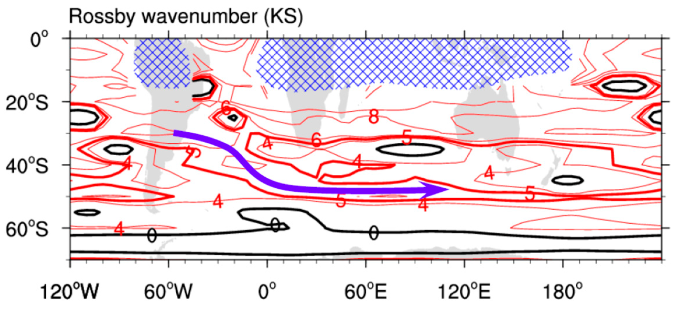
4.1. Waveguide Effect of the Southern Hemisphere Westerly Jet

The two-dimensional horizontal wave-activity flux at 200 hPa related to the SAIO pattern is plotted in Figure 5. An eastward flux is evidenced along the strong Southern Hemisphere westerly jet accompanying the wave train. It diverts northeastward at the exit of the westerly jet at approximately 130° E, and as a result leads to the formation of a positive geopotential height anomaly over Australia, which increases rainfall in Northwest Australia [41] and decreases rainfall in Southeast Australia (Figure 3a). In addition, the eastward flux also curves northeastward at approximately 50° E and extends towards the southwest Indian Ocean, which has also been noticed by DeBlander and Shaman [11].
The zonally oriented wave train over the SAIO is attributable to the waveguide effect of the strong Southern Hemisphere westerly jet. As shown in Figure 6, a local maximum of stationary Rossby wavenumber of 5–6 is illustrated at approximately 45° S over the SAIO where the strong westerly jet prevails (Figure 5). Based on the width of the waveguide, the meridional wavenumber is estimated to be 3. Therefore, the deduced zonal wavenumber of the stationary wave train is about 4, consistent with the wavelength of 90 degrees of the SAIO pattern identified in Figure 2. Because the wave train rays are always refracted towards the latitude with a larger wavenumber, the Rossby wave with the wavenumber less than 5 tends to refract towards the core of the westerly jet. Accordingly, the strong Southern Hemisphere westerly jet acts as an efficient waveguide and traps the eastward-propagating Rossby wave within it forming the SAIO pattern. At the exit of the Southern Hemisphere westerly jet, the local maximum of wavenumber decreases and can no longer trap the SAIO wave train. Most of the SAIO wave train components then divert equatorward to Australia along a great-circle route in the sphere (Figure 5). On the other hand, the equatorward curving of the wave train at approximately 50° E is likely related to the propagation of the Rossby wave with the wavenumber larger than 5, which has been demonstrated by DeBlander and Shaman [11] in Figure 4 based on the analysis of Rossby wave ray tracings. Under this circumstance, the Southern Hemisphere westerly jet cannot trap the short-wavelength wave train components, which propagates northeastward along a great-circle route towards the tropical Indian Ocean (Figure 5).

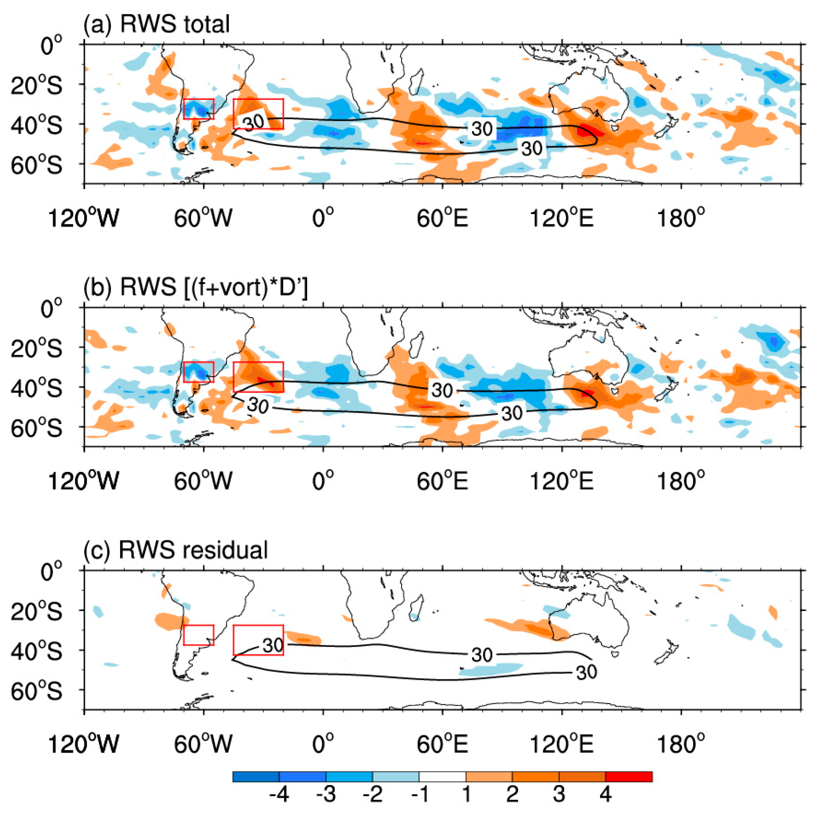
4.2. Anomalous Rossby Wave Source Related to the SAIO Pattern

Since the SAIO pattern shows a nearly barotropic structure (Figure 2), processes that generated the associated anomalies can be understood in a barotropic vorticity equation. For this purpose, the anomalous Rossby wave source (RWS) S is calculated following Sardeshmukh and Hoskins [50]:
S = ( f + ζ ¯ ) V x ζ   V x ¯ V x ( f + ζ ¯ ) V x ¯ ζ
The RWS total related to the SAIO pattern (Figure 7a) distributes mostly in midlatitudes, especially along the belt of the Southern Hemisphere westerly jet. To reveal which process contributes mostly to the RWS total, we further calculated each term in the right hand of the Equation (3). The RWS total is induced mainly by the first term due to the combined impact of the climatological absolute vorticity and anomalous divergence. As shown in Figure 7b, the first term resembles the RWS total (Figure 7a), with a similar spatial pattern and magnitude between them. The residual RWS (the sum of the last three terms, Figure 7c) is much weaker than the first term. The result indicates that the RWS related to the SAIO pattern is determined by the anomalous divergence in the upper troposphere under the climatological basic state.
Sardeshmukh and Hoskins [50] have proposed that RWS can be considered as forcing in generating the Rossby wave pattern. Because the Rossby wave train can only propagate eastward due to the waveguide effect of the Southern Hemisphere westerly jet [13], the SAIO pattern is most likely triggered by the RWS forcing in the upstream region. As shown in Figure 7a, two strong RWSs are identified near the entrance of the westerly jet, with a negative value over mid-latitude South America and a positive value over the southwest South Atlantic in relation to significant in situ convergence and divergence anomalies in the upper troposphere (Figure 8a), respectively. To investigate the possible impact of the two divergent anomalies, we calculated V200 anomalies regressed against the 200-hPa divergences over the two regions. The similar wave train to the SAIO pattern was obtained relating to both the divergent anomalies over mid-latitude South America (Figure 8b) and the southwest South Atlantic (Figure 8c). The correlation coefficients of the PC1 with the divergence anomalies averaged over mid-latitude South America (27.5°–37.5° S, 55°–70° W) and the southwest South Atlantic (22.5°–42.5° S, 20°–45° W) are −0.42 and 0.63, respectively, both significant at the 95% confidence level. Moreover, the divergence anomalies over the two regions are also significantly connected, with a correlation coefficient of −0.55.
To understand the effect of the two mid-latitude divergent anomalies, two realistic divergence forcings are prescribed in a barotropic vorticity equation model described in Section 2, with the divergence value of −1 × 10⁻⁶ s−1 over South America and 1 × 10⁻⁶ s−1 over the southwest South Atlantic. The steady response is presented in Figure 9. Clearly, a mid-latitude zonally oriented wave train is seen over the SAIO in conjunction with the wave-activity flux emanating from the South Atlantic and extending eastward along the westerly jet. The flux diverts northeastward towards the southwest Indian Ocean at approximately 50° E and towards Australia at the exit of the westerly jet, which may reflect the propagation of the Rossby wave trains with the wavenumber being larger and smaller than 5, respectively, triggered by the mid-latitude divergences. The responses are similar to the observed SAIO pattern in relation to the two divergence anomalies (Figure 8b,c). The similarity highlights the importance of the mid-latitude divergence perturbations over South America and the southwest South Atlantic on the formation of SAIO pattern.
The upper-level divergences over mid-latitude South America and the southwest South Atlantic are significantly related to local rainfall anomalies. The divergences correspond to opposite change in rainfall between the two regions. Rainfall increases in mid-latitude South America and decreases in the southwest South Atlantic in relation to the upper-level divergence over the former region (Figure 10a). The reverse rainfall pattern is seen in relation to the divergence over the southwest South Atlantic (Figure 10b). The correlation coefficient between the rainfalls in the two regions is −0.37, significant at the 95% confidence level. Since the two regions are, indeed, located in the west and east of the rainy belt of the South Atlantic Convergence Zone (Figure 10c), the opposite change in rainfall between the two regions, therefore, indicates a zonal shift of the South Atlantic Convergence Zone. Namely, the zonal shift of the South Atlantic Convergence Zone can trigger the SAIO pattern. In addition, the two regions correspond to two regional maxima of rainfall interannual variability (Figure 10c). The strong rainfall/divergence forcing then causes the strong interannual variability of the SAIO pattern (Figure 1). The importance of the rainfall in the South Atlantic Convergence Zone in triggering the mid-latitude wave train has also been suggested by DeBlander and Shaman [11]. They showed a mid-latitude wave train associated with a north–south shift of the South Atlantic Convergence Zone, portion of which is similar to the SAIO pattern. However, they focused more on the induced northward-curving wave train into the tropical Indian Ocean. This study, however, highlights the importance of the east–west shift of the South Atlantic Convergence Zone and the induced zonally oriented wave train along the Southern Hemisphere westerly jet.

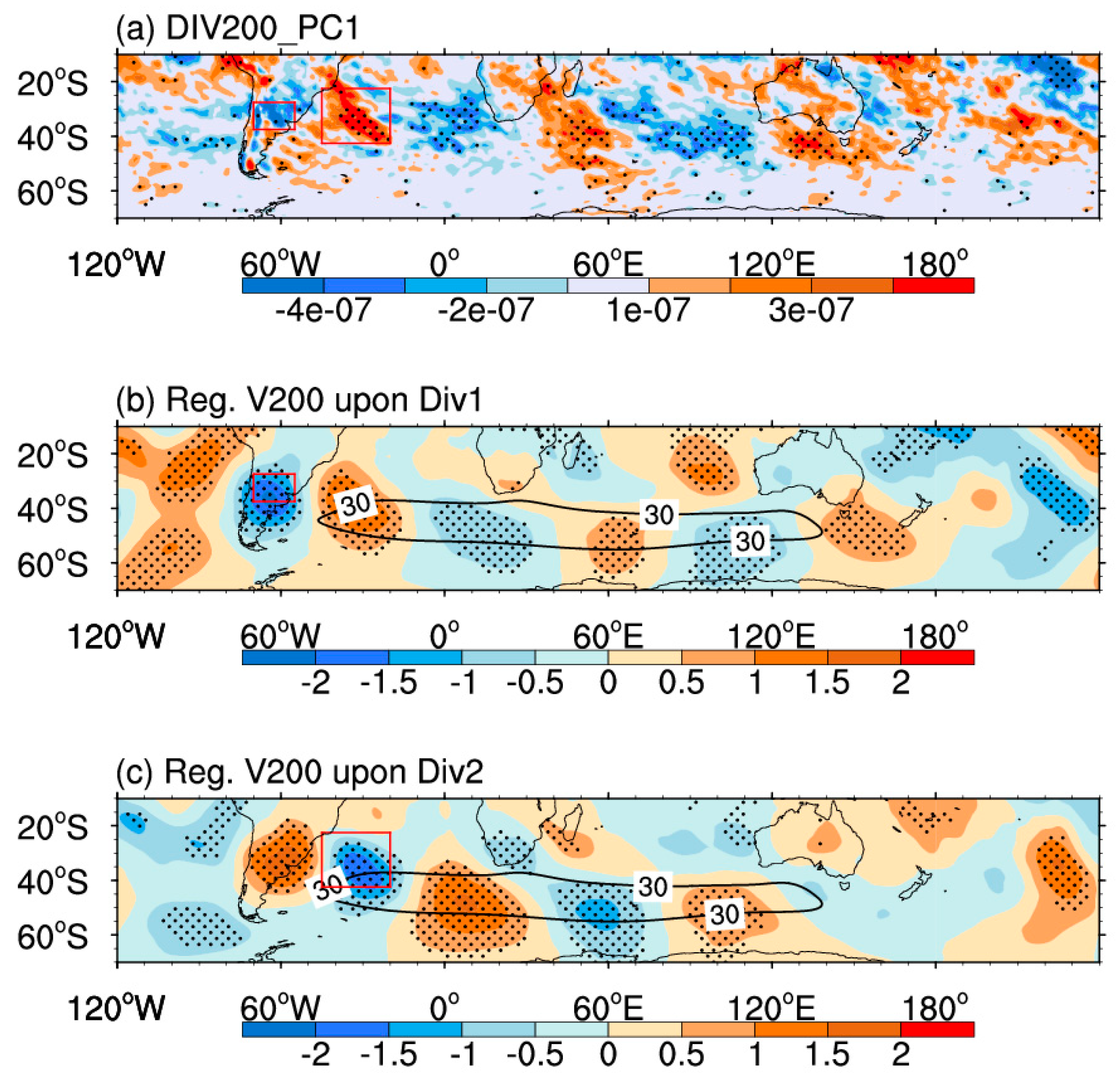
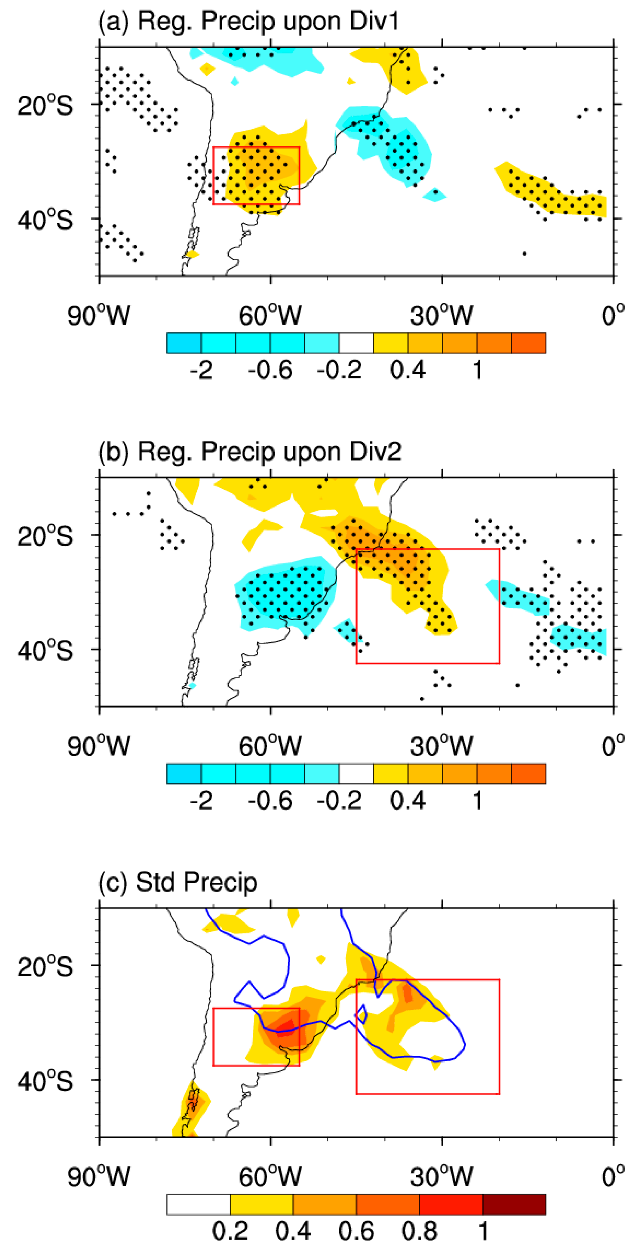
4.3. Tropical Connection of the SAIO Pattern

Some studies have reported the rainfall over mid-latitude South America is related to the tropical SST anomalies [51,52,53]. To see if there is a connection of the SAIO pattern with the tropical external forcing, SST anomalies are regressed against the SAIO index. The regressed SST pattern is similar to the regressed surface air temperature over the oceans in the Southern Hemisphere (Figure 3b), and in the tropical region there is only a weak, negative SST anomaly in the tropical central Pacific east of the dateline (figure not shown). The correlation coefficient between the SAIO index and the Nino3.4 index, which is defined as the mean SST anomaly over the tropical central-eastern Pacific region (5° S–5° N, 120°–170° W), is only −0.2 during 1980–2016. Meanwhile, the correlation is also weak between the Nino3.4 index and the divergences over mid-latitude South America (0.29) and the southwest South Atlantic (–0.21). The result suggests that the SAIO pattern is more likely triggered by the atmosphere internal variability rather than the external SST forcing.
On the other hand, the SAIO pattern does show some significant signals over the tropical eastern Pacific in the upper troposphere (Figure 2a). The tropical relationship of the SAIO pattern is also indicated by a southeastward wave-activity flux from the tropical eastern Pacific (Figure 5). The tropical connection is likely bridged by the upper-tropospheric divergence over mid-latitude South America. After removing the effect of the divergence over South America by subtracting the linear component regressed upon the divergence, the significant tropical signals related to the SAIO pattern, especially to the north of the equator (Figure 2a), diminished (figure not shown). Meanwhile, the tropical signals remain significant after subtracting the effect of the divergence over the southwest South Atlantic (figure not shown). Since the divergence over mid-latitude South America has only a weak connection to the ENSO as discussed above, other tropical process may be responsible for the variations of the divergence over mid-latitude South America. However, this question is beyond the scope of the present study and requires further investigation.

4.4. Relation to the Southern Annular Mode

As identified in Section 3, the SAIO pattern exhibits a hemisphere-scale characteristic. Another circumglobal pattern in the Southern Hemisphere is the Southern Annular Mode (SAM) [54] or Antarctic Oscillation [55]. The two patterns both depict a major variability of mid-latitude atmospheric circulation, in which the SAIO pattern is the first EOF mode of V200 interannual variability in the mid-latitude SAIO and the SAM is the first EOF mode of geopotential height or sea level pressure in the extratropical Southern Hemisphere. Are they connected? To answer the question, we show V200 anomalies regressed upon the SAM index (Figure 11), in which the SAM index is obtained as the principal component corresponding to the first EOF mode of geopotential height at 200 hPa over the extratropical Southern Hemisphere south of 20°S in austral summer following Ding et al. [56].
The SAM mode does show some V200 anomalies over the SAIO region, but the strongest signals are situated in high latitudes and the South Pacific, consistent with the result of Ding et al. [56]. The correlation coefficient of the SAIO index and the SAM index is −0.28, barely significant at the 90% but not at the 95% confidence level. The weak connection is probably bridged by the divergence over mid-latitude South America. The divergence over mid-latitude South America has a significant correlation coefficient of 0.45 with the SAM index, while the correlation between the divergence over the southwest South Atlantic and the SAM index is weak (−0.27). After removing the linear components regressed against the divergence over mid-latitude South America, the correlation between the SAM and the SAIO becomes negligible (−0.11).
We also calculated the correlation of the SAM with the rainfall in the two regions. The correlation coefficients are 0.06 between the SAM and the rainfall over mid-latitude South America and −0.11 over the southwest South Atlantic. Namely, the variations of the mid-latitude rainfall are independent from the SAM. The result confirms, on the other hand, the crucial role of the mid-latitude rainfall in triggering the SAIO pattern independent from the SAM effect.

5. Conclusion and Discussion

This study identifies a teleconnection pattern along the Southern Hemisphere westerly jet over the SAIO. The SAIO pattern depicts a major variability of meridional winds in the upper troposphere over the region. It is barotropic in the vertical direction and with a zonal wavenumber of 4. The SAIO pattern significantly modulates climate variability in the subtropical and mid-latitude Southern Hemisphere in austral summer on the interannual timescales, especially the opposite change in precipitation and surface air temperature between Southeast and Northwest Australia.
The SAIO wave train can be efficiently triggered by divergence perturbations over mid-latitude South America and the southwest South Atlantic, near the entrance of the strong Southern Hemisphere westerly jet, which is probably attributable to the zonal shift of the South Atlantic Convergence Zone. Then, under the waveguide effect of the westerly jet, the signal propagates eastwards within it until in the jet exit at approximately 130° E, where the disturbance escapes and develops northeastward towards Australia, forming the SAIO teleconnection pattern. In addition, portion of the signal also diverts equatorward at approximately 50° E towards the southwest Indian Ocean. Further studies show that the SAIO pattern has a weak connection to the tropical SST anomaly, suggesting that the SAIO pattern is more likely triggered by the atmospheric internal variability rather than external forcing.
This study identified a zonally oriented SAIO pattern along the Southern Hemisphere westerly jet in austral summer. A similar pattern has also been revealed along the Asian westerly jet in boreal summer [16,17,18]. Both patterns are situated within the strong summertime westerly jet waveguide, but they also show some differences, for example, in their spatial pattern (with the zonal wavenumber of 4 in the Southern Hemisphere versus 5 in the Northern Hemisphere) and relationship to tropical SST (significant relationship exists between the tropical Pacific SST and the teleconnection in the Northern Hemisphere but not with the SAIO pattern in the Southern Hemisphere). The comparison between the teleconnections in the two hemispheres may help to better understand the nature of the teleconnections along the westerly jet. However, it is still an open question. In addition, the previous studies have reported there is a mid-latitude wave train along the Southern Hemisphere westerly jet in boreal summer associated with the intraseasonal variation of the MJO [38] and decadal variations of surface air temperature in Australia [43]. This study focuses only on the interannual variations of the SAIO pattern. Variability of the SAIO pattern on the intra-seasonal and decadal timescales and their impacts needs further investigations.

Funding

The research was supported by the Youth Innovation Promotion Association, Chinese Academy of Sciences [grant number 2017105] and by the National Natural Science Foundation of China [grant number 41775062].

Acknowledgments

The author wishes to thank three anonymous reviewers and the editor for their valuable comments. The ERA-Interim data used in this study were downloaded from https://apps.ecmwf.int/datasets/data/interim-full-moda/levtype=pl/ and the CMAP precipitation data from https://www.esrl.noaa.gov/psd/data/gridded/data.cmap.html. All figures were produced using the NCAR Command Language (NCL).

Conflicts of Interest

The author declares that there are no conflict of interest regarding the publication of this paper.

References

  1. Wallace, J.M.; Gutzler, D.S. Teleconnections in the geopotential height field during the northern hemisphere winter. Mon. Weather Rev. 1981, 109, 784–812. [Google Scholar] [CrossRef]
  2. Barnston, A.; Livezey, R. Classification, seasonality and persistence of low-frequency atmospheric circulation patterns. Mon. Weather Rev. 1987, 115, 1083–1126. [Google Scholar] [CrossRef]
  3. Wakabayashi, S.; Kawamura, R. Extraction of major teleconnection patterns possibly associated with the anomalous summer climate in japan. J. Meteorol. Soc. Jpn. 2004, 82, 1577–1588. [Google Scholar] [CrossRef]
  4. Mo, K.C.; Higgins, R.W. The pacific–south american modes and tropical convection during the southern hemisphere winter. Mon. Weather Rev. 1998, 126, 1581–1596. [Google Scholar] [CrossRef]
  5. O’Kane, T.J.; Monselesan, D.P.; Risbey, J.S. A multiscale reexamination of the pacific–south american pattern. Mon. Weather Rev. 2016, 145, 379–402. [Google Scholar] [CrossRef]
  6. Mo, K.C.; Paegle, J.N. The pacific-south american modes and their downstream effects. Int. J. Climatol. 2001, 21, 1211–1229. [Google Scholar] [CrossRef]
  7. Cai, W.; van Rensch, P.; Cowan, T.; Hendon, H.H. Teleconnection pathways of enso and the iod and the mechanisms for impacts on australian rainfall. J. Clim. 2011, 24, 3910–3923. [Google Scholar] [CrossRef]
  8. McIntosh, P.C.; Hendon, H.H. Understanding rossby wave trains forced by the indian ocean dipole. Clim. Dyn. 2018, 50, 2783–2798. [Google Scholar] [CrossRef]
  9. Shimizu, M.H.; de Albuquerque Cavalcanti, I.F. Variability patterns of rossby wave source. Clim. Dyn. 2011, 37, 441–454. [Google Scholar] [CrossRef]
  10. Grimm, A.M.; Reason, C.J.C. Does the south american monsoon influence african rainfall? J. Clim. 2011, 24, 1226–1238. [Google Scholar] [CrossRef]
  11. DeBlander, E.; Shaman, J. Teleconnection between the south atlantic convergence zone and the southern indian ocean: Implications for tropical cyclone activity. J. Geophys. Res. Atmos. 2017, 122, 728–740. [Google Scholar] [CrossRef]
  12. Hoskins, B.J.; Karoly, D.J. The steady linear response of a spherical atmosphere to thermal and orographic forcing. J. Atmos. Sci. 1981, 38, 1179–1196. [Google Scholar] [CrossRef]
  13. Hoskins, B.J.; Ambrizzi, T. Rossby wave propagation on a realistic longitudinally varying flow. J. Atmos. Sci. 1993, 50, 1661–1671. [Google Scholar] [CrossRef]
  14. Hu, K.; Huang, G.; Wu, R.; Wang, L. Structure and dynamics of a wave train along the wintertime asian jet and its impact on east asian climate. Clim. Dyn. 2018, 51, 4123–4137. [Google Scholar] [CrossRef]
  15. Branstator, G. Circumglobal teleconnections, the jet stream waveguide, and the north atlantic oscillation. J. Clim. 2002, 14, 1893–1910. [Google Scholar] [CrossRef]
  16. Lu, R.-Y.; Oh, J.-H.; Kim, B.-J. A teleconnection pattern in upper-level meridional wind over the north african and eurasian continent in summer. Tellus Ser. A 2002, 54, 44–55. [Google Scholar] [CrossRef]
  17. Enomoto, T.; Hoskins, B.J.; Matsuda, Y. The formation mechanism of the bonin high in august. Q. J. R. Meteorol. Soc. 2003, 129, 157–178. [Google Scholar] [CrossRef]
  18. Ding, Q.; Wang, B. Circumglobal teleconnection in the northern hemisphere summer. J. Clim. 2005, 18, 3483–3505. [Google Scholar] [CrossRef]
  19. Huang, G.; Liu, Y.; Huang, R. The interannual variability of summer rainfall in the arid and semiarid regions of northern china and its association with the northern hemisphere circumglobal teleconnection. Adv. Atmos. Sci. 2011, 28, 257–268. [Google Scholar] [CrossRef]
  20. Huang, W.; Feng, S.; Chen, J.; Chen, F. Physical mechanisms of summer precipitation variations in the tarim basin in northwestern china. J. Clim. 2015, 28, 3579–3591. [Google Scholar] [CrossRef]
  21. Li, C.; Wu, L.; Chang, P. A far-reaching footprint of the tropical pacific meridional mode on the summer rainfall over the yellow river loop valley. J. Clim. 2010, 24, 2585–2598. [Google Scholar] [CrossRef]
  22. Small, D.; Islam, S.; Barlow, M. The impact of a hemispheric circulation regime on fall precipitation over north america. J. Hydrometeorol. 2010, 11, 1182–1189. [Google Scholar] [CrossRef]
  23. Syed, F.; Yoo, J.; Körnich, H.; Kucharski, F. Extratropical influences on the inter-annual variability of south-asian monsoon. Clim. Dyn. 2012, 38, 1661–1674. [Google Scholar] [CrossRef]
  24. Zhu, W.; Zhang, Y. Summertime atmospheric teleconnection pattern associated with a warming over the eastern tibetan plateau. Adv. Atmos. Sci. 2009, 26, 413–422. [Google Scholar] [CrossRef]
  25. Chen, G.; Huang, R. Excitation mechanisms of the teleconnection patterns affecting the july precipitation in northwest china. J. Clim. 2012, 25, 7834–7851. [Google Scholar] [CrossRef]
  26. Hong, X.; Lu, R.; Li, S. Amplified summer warming in europe–west asia and northeast asia after the mid-1990s. Environ. Res. Lett. 2017, 12, 094007. [Google Scholar] [CrossRef]
  27. Lin, Z.; Lu, R.; Wu, R. Weakened impact of the indian early summer monsoon on north china rainfall around the late 1970s. J. Clim. 2017, 30, 7991–8005. [Google Scholar] [CrossRef]
  28. Li, X.; Lu, R. Extratropical factors affecting the variability in summer precipitation over the yangtze river basin, china. J. Clim. 2017, 30, 8357–8374. [Google Scholar] [CrossRef]
  29. Lin, Z. Intercomparison of impacts of four summer teleconnections over eurasia on east asian rainfall. Adv. Atmos. Sci. 2014, 31, 1366–1376. [Google Scholar] [CrossRef]
  30. Yu, B.; Lin, H.; Soulard, N. A comparison of north american surface temperature and temperature extreme anomalies in association with various atmospheric teleconnection patterns. Atmosphere 2019, 10, 172. [Google Scholar] [CrossRef]
  31. Wu, R. Relationship between indian and east asian summer rainfall variations. Adv. Atmos. Sci. 2017, 34, 4–15. [Google Scholar] [CrossRef]
  32. Wu, R. A mid-latitude asian circulation anomaly pattern in boreal summer and its connection with the indian and east asian summer monsoons. Int. J. Climatol. 2002, 22, 1879–1895. [Google Scholar] [CrossRef]
  33. Ambrizzi, T.; Hoskins, B.J.; Hsu, H.H. Rossby wave propagation and teleconnection patterns in the austral winter. J. Atmos. Sci. 1995, 52, 3661–3672. [Google Scholar] [CrossRef]
  34. Risbey, J.S.; O’Kane, T.J.; Monselesan, D.P.; Franzke, C.L.E.; Horenko, I. On the dynamics of austral heat waves. J. Geophys. Res. Atmos. 2018, 123, 38–57. [Google Scholar] [CrossRef]
  35. Müller, G.V.; Ambrizzi, T. Teleconnection patterns and rossby wave propagation associated to generalized frosts over southern south america. Clim. Dyn. 2007, 29, 633–645. [Google Scholar] [CrossRef]
  36. Reeder, M.J.; Spengler, T.; Musgrave, R. Rossby waves, extreme fronts, and wildfires in southeastern australia. Geophys. Res. Lett. 2015, 42, 2015–2023. [Google Scholar] [CrossRef]
  37. Tozer, C.R.; Risbey, J.S.; O’Kane, T.J.; Monselesan, D.P.; Pook, M.J. The relationship between wave trains in the southern hemisphere storm track and rainfall extremes over tasmania. Mon. Weather Rev. 2018, 146, 4201–4230. [Google Scholar] [CrossRef]
  38. Zhao, C.; Li, T.; Zhou, T. Precursor signals and processes associated with mjo initiation over the tropical indian ocean. J. Clim. 2012, 26, 291–307. [Google Scholar] [CrossRef]
  39. Fauchereau, N.; Trzaska, S.; Richard, Y.; Roucou, P.; Camberlin, P. Sea-surface temperature co-variability in the southern atlantic and indian oceans and its connections with the atmospheric circulation in the southern hemisphere. Int. J. Climatol. 2003, 23, 663–677. [Google Scholar] [CrossRef]
  40. Jury, M.R.; Parker, B.A.; Raholijao, N.; Nassor, A. Variability of summer rainfall over madagascar: Climatic determinants at interannual scales. Int. J. Climatol. 1995, 15, 1323–1332. [Google Scholar] [CrossRef]
  41. Lin, Z.; Li, Y. Remote influence of the tropical atlantic on the variability and trend in north west australia summer rainfall. J. Clim. 2012, 25, 2408–2420. [Google Scholar] [CrossRef]
  42. Grimm, A.M.; Reason, C.J.C. Intraseasonal teleconnections between south america and south africa. J. Clim. 2015, 28, 9489–9497. [Google Scholar] [CrossRef]
  43. Xue, J.; Li, J.; Sun, C.; Zhao, S.; Mao, J.; Dong, D.; Li, Y.; Feng, J. Decadal-scale teleconnection between south atlantic sst and southeast australia surface air temperature in austral summer. Clim. Dyn. 2018, 50, 2687–2703. [Google Scholar] [CrossRef]
  44. Dee, D.; Uppala, S.; Simmons, A.; Berrisford, P.; Poli, P.; Kobayashi, S.; Andrae, U.; Balmaseda, M.; Balsamo, G.; Bauer, P. The era-interim reanalysis: Configuration and performance of the data assimilation system. Q. J. R. Meteorol. Soc. 2011, 137, 553–597. [Google Scholar] [CrossRef]
  45. Xie, P.P.; Arkin, P.A. Global precipitation: A 17-year monthly analysis based on gauge observations, satellite estimates, and numerical model outputs. Bull. Am. Meteorol. Soc. 1997, 78, 2539–2558. [Google Scholar] [CrossRef]
  46. Takaya, K.; Nakamura, H. A formulation of a phase-independent wave-activity flux for stationary and migratory quasigeostrophic eddies on a zonally varying basic flow. J. Atmos. Sci. 2001, 58, 608–627. [Google Scholar] [CrossRef]
  47. North, G.R.; Bell, T.L.; Cahalan, R.F.; Moeng, F.J. Sampling errors in the estimation of empirical orthogonal functions. Mon. Weather Rev. 1982, 110, 699–706. [Google Scholar] [CrossRef]
  48. Kalnay, E.; Kanamitsu, M.; Kistler, R.; Collins, W.; Deaven, D.; Gandin, L.; Iredell, M.; Saha, S.; White, G.; Woollen, J. The ncep/ncar 40-year reanalysis project. Bull. Am. Meteorol. Soc. 1996, 77, 437–471. [Google Scholar] [CrossRef]
  49. Timbal, B.; Fawcett, R. A historical perspective on southeastern australian rainfall since 1865 using the instrumental record. J. Clim. 2013, 26, 1112–1129. [Google Scholar] [CrossRef]
  50. Sardeshmukh, P.D.; Hoskins, B.J. The generation of global rotational flow by steady idealized tropical divergence. J. Atmos. Sci. 1988, 45, 1228–1251. [Google Scholar] [CrossRef]
  51. Paegle, J.N.; Mo, K.C. Linkages between summer rainfall variability over south america and sea surface temperature anomalies. J. Clim. 2002, 15, 1389–1407. [Google Scholar] [CrossRef]
  52. Zhou, J.; Lau, K.M. Principal modes of interannual and decadal variability of summer rainfall over south america. Int. J. Climatol. 2001, 21, 1623–1644. [Google Scholar] [CrossRef]
  53. Montecinos, A.; Díaz, A.; Aceituno, P. Seasonal diagnostic and predictability of rainfall in subtropical south america based on tropical pacific sst. J. Clim. 2000, 13, 746–758. [Google Scholar] [CrossRef]
  54. Thompson, D.W.J.; Wallace, J.M. Annular modes in the extratropical circulation. Part i: Month-to-month variability. J. Clim. 2000, 13, 1000–1016. [Google Scholar] [CrossRef]
  55. Gong, D.; Wang, S. Definition of antarctic oscillation index. Geophys. Res. Lett. 1999, 26, 459–462. [Google Scholar] [CrossRef]
  56. Ding, Q.; Steig, E.J.; Battisti, D.S.; Wallace, J.M. Influence of the tropics on the southern annular mode. J. Clim. 2012, 25, 6330–6348. [Google Scholar] [CrossRef]
Figure 1. Basic features of meridional winds at 200 hPa (V200, unit: m s−1) over 30°–70° S, 50° W–150° E in austral summer (December-January-February-March, DJFM): (a) standard deviation, (b) the first EOF (EOF 1) mode, (c) one-point correlation of V200 for the reference location (46.5° S, 5.25° E) depicted by the filled black circle, and (d) the principal component corresponding to the EOF1 mode (PC1). Black contour in (a) depicts the climatological Southern Hemisphere westerly jet with zonal wind at 200 hPa exceeding 30 m s−1 and in (c) represents significance at the 95% confidence level based on Student’s t-test. The EOF 1 mode explains 28% of total interannual variance.
Atmosphere 10 00259 g001
Figure 2. Anomalies of meridional winds (unit: m s−1) at (a) 200hPa, (b) 500hPa, and (c) 850 hPa regressed upon the PC1. Locations with significant anomalies at the 95% confidence level based on Student’s t-test are dotted, and the contour in (a) depicts the Southern Hemisphere westerly jet as in Figure 1a. The associated wave train, which is mainly located over the South Atlantic and South Indian Ocean (SAIO), is referred to as the SAIO pattern and the PC1 in Figure 1d as the SAIO index.
Atmosphere 10 00259 g002
Figure 3. As in Figure 2, but for anomalies of (a) precipitation (unit: mm d−1) and (b) surface air temperature (unit: K) associated with the SAIO pattern, which is obtained through regressing upon the PC1.
Atmosphere 10 00259 g003
Figure 4. Anomalies of horizontal winds (vector, m s−1) and its divergence (shading, s−1) at (a) 200 hPa and (c) 850 hPa, and (b) pressure vertical velocity at 500 hPa (Pa s−1) associated with the SAIO pattern.
Atmosphere 10 00259 g004
Figure 5. As in Figure 2a, but for anomalies of geopotential height at 200 hPa (shading, unit: gpm) and related wave-activity flux (vector, unit: m2 s−2).
Atmosphere 10 00259 g005
Figure 6. Total wavenumber of stationary Rossby wave (KS) at the 200 Pa in austral summer. Contours are drawn at 0, 4, 5, 6, 8, 10, 15, and 20. The contour for wavenumber 0 (where the Rossby wave is refracted) is drawn in black, and the rest are in red. The hatched areas depict the regions of climatological easterly averaged over 1980–2016, and the arrow for the Southern Hemisphere westerly jet waveguide with the maximal KS larger than 5 by the thick red contour.
Atmosphere 10 00259 g006
Figure 7. (a) Rossby wave source (RWS, unit: 10−11 s−2) total, (b) RWS induced directly by anomalous divergence, and (c) the residual RWS associated with the SAIO pattern. See text for more details. The boxes depict the two key forcing regions for the SAIO pattern and the contour depicts the Southern Hemisphere westerly jet.
Atmosphere 10 00259 g007
Figure 8. (a) As in Figure 2a, but for anomalies of divergence (unit: s−1) at 200 hPa regressed upon the SAIO pattern. (bc) Anomalies of V200 regressed upon the 200-hPa divergence over (b) mid-latitude South America (Div1, 27.5°–37.5° S, 55°–70° W) and (c) the southwest South Atlantic (Div2, 22.5°–42.5° N, 20°–45° W) depicted by the box. Dotted regions denote that the anomalies are significant at the 95% confidence level based on Student’s t-test and the contour depicts the Southern Hemisphere westerly jet.
Atmosphere 10 00259 g008
Figure 9. Response of rotational meridional winds (shading) and associated wave-activity flux (vector), averaged over the model day 30–60, in a linear barotropic vorticity equation model. The barotropic vorticity equation was linearized about the ERA-Interim reanalysis 200-hPa DJFM streamfunction climatology averaged over 1980–2016. Divergent forcing was applied over mid-latitude South America (27.5°–37.5° S, 55°–70° W) and the southwest South Atlantic (22.5°–42.5° N, 20°–45° W), depicted by the two boxes, with the divergence forcing of −1 × 10 −6 s−1 and 1 × 10⁻⁶ s−1, respectively. Contour depicts climatological zonal winds at 200 hPa.
Atmosphere 10 00259 g009
Figure 10. (a,b) As in Figure 8b,c, but for anomalies of precipitation. (c) Standard deviation of austral summer rainfall (unit: mm d−1), in which the zonal mean is removed. The two boxes depict mid-latitude South America and the southwest South Atlantic. The blue contour represents the climatological rainy belt of the South Atlantic Convergence zone, with mean rainfall averaged over 1980–2016 exceeding 2 mm d−1 using the CMAP precipitation data.
Atmosphere 10 00259 g010
Figure 11. As in Figure 2a, but for anomalies of V200 associated with the SAM mode, which is represented by the EOF 1 mode of extratropical geopotential height at 200 hPa south of 20° S in austral summer.
Atmosphere 10 00259 g011

